Absolute dimensions of detached eclipsing binaries. III. The metallic-lined system YZ Cassiopeiae

Abstract

The bright binary system YZ Cassiopeiae is a remarkable laboratory for studying the Am phenomenon. It consists of a metallic-lined A2 star and an F2 dwarf on a circular orbit, which undergo total and annular eclipses. We present an analysis of 15 published light curves and 42 new high-quality échelle spectra, resulting in measurements of the masses, radii, effective temperatures and photospheric chemical abundances of the two stars. The masses and radii are measured to 0.5% precision: $M_{\rm A}=2.263\pm 0.012$$\,{\rm M}_{\odot}$, $M_{\rm B}=1.325\pm 0.007$$\,{\rm M}_{\odot}$, $R_{\rm A}=2.525\pm 0.011$$\,{\rm R}_{\odot}$ and $R_{\rm B}=1.331\pm 0.006$$\,{\rm R}_{\odot}$. We determine the abundance of 20 elements for the primary star, of which all except scandium are super-solar by up to 1 dex. The temperature of this star ($9520\pm 120$ K) makes it one of the hottest Am stars. We also measure the abundances of 25 elements for its companion ($T_{\rm eff}=6880\pm 240$ K), finding all to be solar or slighly above solar. The photospheric abundances of the secondary star should be representative of the bulk composition of both stars. Theoretical stellar evolutionary models are unable to match these properties: the masses, radii and temperatures imply a half-solar chemical composition ($Z=0.009\pm 0.003$) and an age of 490–550 Myr. YZ Cas therefore presents a challenge to stellar evolutionary theory.

1 Introduction

Eclipsing binary star systems are of fundamental importance to astrophysics as they are the primary source of direct measurements of the physical properties of stars (Andersen, 1991; Torres et al., 2010). The masses and radii of double-lined systems can be measured to precisions of better than 1% using only geometric arguments (e.g. Clausen et al., 2008). Obtaining effective temperature ($T_{\rm eff}$) measurements converts them into excellent distance indicators (Ribas et al., 2005; Bonanos et al., 2006). Detached eclipsing binaries (dEBs) hold an additional advantage as their properties can be used to investigate the predictive abilities of evolutionary models for single stars.

Metallic-lined A stars (Am stars) are defined to be those which show unusually weak Ca and/or Sc lines and overly strong metallic lines for their spectral type as derived from Balmer line profiles (Conti, 1970; Gray & Corbally, 2009). They were first described as a class of chemically peculiar stars by Titus & Morgan (1940). Their abundance anomalies are explained as the product of chemical stratification caused by radiative levitation and gravitational settling (Michaud, 1970; Turcotte et al., 2000; Talon et al., 2006). Pulsations have recently been found in many Am stars (Smalley et al., 2011; Balona et al., 2011).

These physical phenomena can produce observable effects in quiet radiative atmospheres. The Am phenomenon occurs only in stars with rotational velocities slower than about 100 km s^-1 (Abt & Levy, 1985; Budaj, 1996, 1997). Am stars are preferentially found in binary systems, where tidal effects cause a slower rotation than for single stars (Abt, 1961, 1965; Carquillat & Prieur, 2007). This means that they are well-represented in the known population of dEBs , for example V364 Lac (Torres et al., 1999), V459 Cas (Lacy et al., 2004), WW Cam (Lacy et al., 2002) and RR Lyn (Tomkin & Fekel, 2006). Whilst the Am phenomenon is a ‘surface disease’, a very high bulk metal abundance was found for the metallic-lined dEB WW Aur by Southworth et al. (2005c).

In this work we present a detailed analysis of the dEB YZ Cas, a system which consists of a metallic-lined A2 star and an F2 dwarf of significantly lower mass, radius and $T_{\rm eff}$. This system provides an opportunity to study the Am phenomenon in a star for which the internal chemical composition can be inferred – from its lower-mass companion. YZ Cas is particularly well suited to such an analysis. It is totally eclipsing and extensive photometric data is available in the literature, so the radii of the stars can be determined to unusually high precision. It is also bright and contains slowly rotating stars, making spectroscopic analysis especially productive. Below we recap the long observational history of this object, model the available light curves, analyse new échelle spectroscopy of the system, deduce the physical properties of the two stars, and finally confront theoretical models with our results.

1.1 YZ Cassiopeiae

Table 1: Identifications, location, and combined photometric indices for YZ Cassiopeiae.

		YZ Cassiopeiae	Reference
Flamsteed designation		21 Cas	1
Hipparcos number		HIP 3572	2
Henry Draper number		HD 4161	3
Bright Star Catalogue		HR 192	4
Bonner Durchmusterung		BD +74 27	5
$\alpha_{2000}$		00 45 39.078	2
$\delta_{2000}$	+	74 59 17.06	2
Hipparcos parallax ($m$as)		11.24 $\pm$ 0.55	2
Spectral type		A2m + F2V	6
$B_{T}$		5.739 $\pm$ 0.003	2
$V_{T}$		5.660 $\pm$ 0.003	2
$J_{\rm 2MASS}$		5.585 $\pm$ 0.019	7
$H_{\rm 2MASS}$		5.644 $\pm$ 0.038	7
$K_{\rm 2MASS}$		5.602 $\pm$ 0.021	7
$b-y$		0.036 $\pm$ 0.005	8
$v-b$		0.211 $\pm$ 0.007	8
$u-b$		1.455 $\pm$ 0.008	8

References: (1) Flamsteed (1712); (2) Perryman et al. (1997); (3) Cannon & Pickering (1918); (4) Hoffleit & Jaschek (1991); (5) Argelander (1903); (6) This work; (7) 2MASS (Cutri et al., 2003); (8) Hilditch & Hill (1975), given as the mean and standard deviation of the six measurements for each Strömgren colour index (all taken outside eclipse).

YZ Cas shows total and annular eclipses recurring on an orbital period of 4.47 d. It has been the subject of many analyses over nearly a century, which we summarise below. Throughout this work we refer to the primary component as star A and the secondary component as star B. Star A is substantially hotter, larger and more massive than star B, and is the component in inferior conjunction at the midpoint of primary eclipse. The spectral type of the YZ Cas system is given as A2 in the Henry Draper Catalogue (Cannon & Pickering, 1918); this measurement pertains to star A, which dominates the light of the system.

The eclipsing nature of YZ Cas was announced by Stebbins (1924), who is credited with the discovery, and further elaborated by Huffer (1925). It was chosen at the Washburn Observatory as a photometric comparison star for 23 Cas (a spectroscopic binary which has not been observed to be variable). The resulting light curve was presented by Huffer (1928).

Plaskett (1926) determined the first spectroscopic orbit of the system, based on radial velocity (RV) measurements of star A. Under the assumption that both stars had a mass of 2$\,{\rm M}_{\odot}$ he measured their radii and orbital separation. Plaskett detected the Rossiter-McLaughlin effect (Rossiter, 1924; McLaughlin, 1924) during primary minimum, with an amplitude slightly greater than 3 km s^-1. The shape of the Rossiter-McLaughlin anomaly is consistent with alignment between the orbital and stellar rotational axes, albeit with low significance.

Kron (1939b) used the annular nature of secondary eclipse to measure the colour index of star B, based on photoelectric photometry from Huffer (1931), and transformed this into an approximate spectral type of F4.

Kron (1939a) presented and tabulated a light curve of the system with full coverage of the eclipses, obtained using a photoelectric photometer with an effective wavelength of 4500 Å (Kron, 1939c). He used this to measure the fractional radii and limb darkening (LD) coefficients of the two stars (see also Kron, 1938). Kron (1942) used the same instrument but with a red filter and red-sensitive light detector to obtain a second light curve in a passband covering 5200–8200 Å (half maximum response). He found fractional radii in good agreement with those from his blue light curve, and determined a colour of star B corresponding to a spectral type of F5. Serkowski (1961) reconsidered the determination of the LD coefficients from the Kron light curves.

McNamara (1951) presented two new light curves in a blue and a UV passband, obtained using similar equipment and methods to Kron (1939a). The main aim was to investigate the LD at blue wavelengths. Grygar et al. (1972) presented a detailed discussion of LD from the two Kron and the two McNamara light curves, and revised measurements of the physical properties of the stars.

Koch et al. (1965) measured the spectral type of star A to be A2-A3 and its equatorial rotational velocity to be $V_{\rm eq}=34\pm 2$ km s^-1. Perry & Stone (1966) obtained a single-lined spectroscopic orbit from 92 RVs. Their measured orbital eccentricity, $e=0.004\pm 0.004$ (most likely a probable rather than standard error), suggests that the orbit is circular (Lucy & Sweeney, 1971).

Lacy (1981) studied YZ Cas using the Kron light curves and new spectra from which RVs were measured for star B for the first time. Lacy adopted photometric parameters which were the weighted average of eight independent studies of the same light curves (Kron, 1939a, 1942), a procedure which may lack statistical validity. Lacy also obtained individual Strömgren photometric indices of the two component stars from published photometry. Lacy’s RVs yielded measurements of the masses of the stars to a precision of 0.5%, allied with values of $V_{\rm eq}$ of $34\pm 1$ km s^-1 for star A and $16\pm 2$ km s^-1 for star B.

Shortly after publication of the study of Lacy (1981), de Landtsheer (1983) presented a large number of photoelectric observations of YZ Cas. These were obtained in four colours in the Utrecht photometric system (Provoost, 1980; Heintze & Van Gent, 1989), and were analysed using the code of Wilson & Devinney (1971) in order to obtain the physical properties of the stars. de Landtsheer & Mulder (1983) obtained two high-resolution UV spectra from the International Ultraviolet Explorer satellite and confirmed the metallic nature of star A. The abundance of star B was not measured, so the internal (rather than photospheric) abundance of star A remained unknown. de Landtsheer & De Greve (1984) found a subsolar metal abundance ($Z=0.015$ where $Z$ is the mass fraction of metals) in a comparison with theoretical stellar evolutionary models, in disagreement with Lacy’s finding of a supersolar bulk metal abundance of $Z=0.027\pm 0.003$.

Finally, Papoušek (1989) obtained 16 000 photoelectric observations in six passbands, from the 60 cm reflector of the University Observatory, Brno. He used these to study the physical properties and LD of the system.

2 Observations and data reduction

2.1 Spectroscopy

We obtained 42 high-resolution spectra of YZ Cas in October 2007, using the Nordic Optical Telescope (NOT) at La Palma, Spain, equipped with the FIbre-fed Echelle Spectrograph (FIES). This spectrograph is housed in a separate climate-controlled building and has a high thermal and mechanical stability. The wavelength scale was established from thorium-argon exposures taken regularly throughout the observing nights. We used fibre 4 in fibre bundle B, giving complete spectral coverage in the interval 3640–7360 Å at a reciprocal dispersion ranging from 0.023 Å px^-1 in the blue to 0.045 Å px^-1 in the red. The resolution of the instrument is roughly 3.5 px, giving a resolving power of 48 000. An exposure time of 300 s was used for all spectra, resulting in continuum signal to noise ratios in the region of 300 in the $B$ and $V$ bands.

The basic steps for data reduction (bias subtraction, flat-fielding, correction for scattered light, extraction of orders, and wavelength calibration) were performed with IRAF. Removal of the instrumental blaze function for YZ Cas is not trivial, because the broad Balmer lines from star A extend over entire échelle orders. In such cases we interpolated blaze functions from adjacent orders which are well-defined, using a semi-manual approach and java routines written by VK.

2.2 Photometry

Table 2: The wavelengths of maximum transmission ($\lambda_{\rm cen}$) and the full widths at half maximum response (FWHM) of the passbands of the light curves used in this work. When possible the FWHM is given as the actual wavelength interval rather than just the width of the passband.

Passband	$\lambda_{\rm cen}$ (Å)	FWHM (Å)	Reference
Kron blue	4500	(wide)	Kron (1939c)
Kron red	6000	5250–8220	Kron (1942)
McNamara UV	3575	850	McNamara (1951)
McNamara blue	4525	3500–5700	McNamara (1951)
Utrecht 472	4730	105	Provoost (1980)
Utrecht 672	6719	100	Provoost (1980)
Utrecht 782	7812	115	Provoost (1980)
Utrecht 871	8798	130	Provoost (1980)
U1	3500	260	Papoušek (1989)
U2	3810	155	Papoušek (1989)
B	4075	190	Papoušek (1989)
G	4903	100	Papoušek (1989)
V	5405	145	Papoušek (1989)
O	5822	100	Papoušek (1989)
Hipparcos	4800	4280–6550	Bessell (2000)

We present no new photometry in this work, due to the large number and good quality of existing datasets. Published observations were taken from a range of sources, discussed in Sect. 1.1, resulting in a total of 15 separate light curves. All of these were observed in non-standard passbands, so we give a summary of them in Table 2. We did not use the data from Huffer (1928) as they are sparse and relatively scattered.

Kron (1939a) and Kron (1942) presented photoelectric photometry of YZ Cas in one blue and one red wide passband, obtained using a 1 m reflector at the Lick Observatory. The two Kron light curves were obtained from the papers by optical character recognition using the tesseract software. Due to changes in the optical path of the instrument between the variable star and its comparison star (23 Cas), many of the nights of data were shifted in magnitude to obtain a good internal agreement. Becase of this, the observations taken well outside eclipse carry essentially no information. We have therefore rejected data taken more than 0.05 phase units from the midpoint of an eclipse. A few observations were enclosed in square brackets to indicate that they are less reliable, and we also rejected these. Each Kron datapoint is the sum of six individual deflections on the chart recorder, meaning they have a relatively high precision.

McNamara (1951) observed YZ Cas in one UV and one blue passband, with central wavelengths of 3575 Å and 4525 Å for an A0 star. The UV passband was selected using a Corning O-5840 glass filter, and the blue passband with Corning C-5562 and O-3389 glass. The passband widths were not specified by McNamara (1951), so have been obtained from diagrams in Dobrowolski et al. (1977) and are given in Table 2. The blue passband has more than 50% transmission from $4300\pm 50$ Å to $5700\pm 150$ Å, but a long red tail of roughly 30% transmission extends beyond the edge of Fig. 20 in Dobrowolski et al. (1977) at 7500 Å. The photometric data were obtained from McNamara (1951) as a function of orbital phase.

de Landtsheer (1983) obtained light curves of YZ Cas in four different narrow passbands in the Utrecht photometric system, centred on wavelengths 474, 672, 782 and 871 nm. These were aimed at wavelength intervals containing no telluric lines and the fewest stellar spectral lines possible, with the motivation of improving the understanding of continuum LD through study of dEBs. Only one set of Utrecht filters is known to exist, and these were affixed to a 40 cm reflector then operated at Ausserbin in the Swiss Alps. The four Utrecht light curves had to be obtained from the paper by copying out by hand. They have a much larger scatter than the Kron data, but the morphology of the light variation of YZ Cas means they are still valuable data.

YZ Cas was bright enough to be observed by the Hipparcos satellite (Perryman et al., 1997) and also the Tycho experiment on board Hipparcos (Høg et al., 1997). All three datasets suffer from a shortage of points within the total phases of secondary minimum, but in the case of the Hipparcos passband the scatter is sufficiently small that the points on the ascending branch of the secondary minimum provide adequate constraints on the depth of the minimum.

Papoušek (1989) presented possibly the most extensive observations of YZ Cas. These comprise about 16 000 observations in an intermediate-band filter system denoted $U1$, $U2$, $B$, $G$, $V$ and $O$, in order of increasing wavelength. These are tabulated in his paper as sets of normal points covering phases between 0 and 1, and were converted into machine-readable format using tesseract. As they are specified as magnitudes versus phase we do not have information on the times of individual observations, only that the data were obtained in the years 1973–1974.

3 Orbital period determination

Table 3: Literature times of minimum light of YZ Cas and the observed minus calculated ($O-C$) values of the data compared to the ephemeris derived in this work.

Time of minimum	Cycle	$O-C$ value	Reference
(HJD $-$ 2 400 000)	number	(HJD)
23716.7318 $\pm$ 0.01	$-$4895.0	$-$0.00136	1
23966.8931 $\pm$ 0.005	$-$4839.0	$-$0.00452	2
23975.8282 $\pm$ 0.003	$-$4837.0	$-$0.00386	3
25374.070 $\pm$ 0.005	$-$4524.0	$-$0.00266	1
25414.274 $\pm$ 0.01	$-$4515.0	$-$0.00366	1
25512.568 $\pm$ 0.01	$-$4493.0	0.01144	4
25776.122 $\pm$ 0.01	$-$4434.0	$-$0.00068	4
26562.354 $\pm$ 0.01	$-$4258.0	0.00019	4
26754.443 $\pm$ 0.005	$-$4215.0	$-$0.00137	5
26763.386 $\pm$ 0.005	$-$4213.0	0.00718	5
26946.5317 $\pm$ 0.005	$-$4172.0	$-$0.00324	6
26955.4548 $\pm$ 0.005	$-$4170.0	$-$0.01458	6
26973.357 $\pm$ 0.005	$-$4166.0	0.01873	5
28733.4218 $\pm$ 0.003	$-$3772.0	$-$0.00208	7
29175.6774 $\pm$ 0.005	$-$3673.0	$-$0.00150	8
41355.5615 $\pm$ 0.0019	$-$946.5	0.00082	9
41880.45922 $\pm$ 0.00020	$-$829.0	$-$0.00009	10
42148.49266 $\pm$ 0.00010	$-$769.0	0.00001	10
43256.3644 $\pm$ 0.0003	$-$521.0	0.00060	9
44632.2678 $\pm$ 0.0005	$-$213.0	$-$0.00049	9
44632.2685 $\pm$ 0.0010	$-$213.0	0.00021	11
44929.3378 $\pm$ 0.0009	$-$146.5	$-$0.00078	9
45583.7863 $\pm$ 0.0009	0.0	$-$0.00035	12
45583.7867 $\pm$ 0.0004	0.0	0.00005	12
45621.748 $\pm$ 0.005	8.5	$-$0.01004	12
45621.756 $\pm$ 0.004	8.5	$-$0.00204	12
45990.297 $\pm$ 0.004	91.0	$-$0.00689	12
45990.305 $\pm$ 0.006	91.0	0.00111	12
48411.53820 $\pm$ 0.00056	633.0	$-$0.00020	13
48411.5384 $\pm$ 0.0032	633.0	0.00000	13
48411.5372 $\pm$ 0.0030	633.0	$-$0.00120	13
48822.5201 $\pm$ 0.003	725.0	$-$0.00277	14
54509.2969 $\pm$ 0.0003	1998.0	$-$0.00004	15

References: (1) Kukarkin (1928); (2) Plaskett (1926); (3) Huffer (1931); (4) Zverev (1936); (5) Hassenstein (1954); (6) Skoberla (1936); (7) Kron (1939a); (8) Dombrovskij (1964); (9) Lavrov & Lavrova (1988); (10) Papoušek (1989); (11) de Landtsheer (1983); (12) Diethelm & Lines (1986); (13) This work, based on the Hipparcos and Tycho $B$ and $V$ observations; (14) Brelstaff (1994); (15) P. Svoboda (in Brát et al. 2008).

The available times of minimum light for YZ Cas extend from 1923 to 2008. Most of these are listed by Kreiner et al. (2001) and Papoušek (1989), to which we added a few additional values from a literature search. We rejected several recent visual timings which were either discrepant or too uncertain to be useful. A straight line was fitted to these timings as a function of HJD, from which we determined the orbital ephemeris:

$${\rm Min\,I}={\rm HJD}\ 2\,445\,583.78664(10)+4.46722236(11)\times E$$

The individual times of minimum light are given in Table 3 along with their references and residuals versus the fitted ephemeris. The time system used in this work is UTC, which does not compensate for leap seconds; the time of primary eclipse is only specified to within 9 s so this does not have a significant effect on the results.

A small number of timings refer to secondary rather than primary minimum. We assumed these to represent phase 0.5, and their residuals support this assumption. The minimum timings are therefore consistent with a circular orbit.

4 Light curve analysis

The 15 available light curves of YZ Cas have been individually modelled using the jktebop code code (Southworth et al., 2004a; Southworth, 2013), which is based on the ebop program developed by P. B. Etzel (Popper & Etzel, 1981; Etzel, 1981; Nelson & Davis, 1972). This code represents the stellar figures as biaxial spheroids, with the spherical approximation used for the calculation of eclipse functions. This approximation is more than adequate for well-detached EBs such as YZ Cas. Tests for third light and orbital eccentricity returned small and insignificant values, so these parameters were held at zero for the final solutions. The orbital period was fixed at the value found in Sect. 3, but the ephemeris zeropoint was included as a fitted parameter. The brightness outside eclipse was fitted for, as were the sum and ratio of the fractional radii ($r_{\rm A}+r_{\rm B}$ and $k$), the orbital inclination ($i$), and the central surface brightness ratio of the stars ($J$).

YZ Cas has a rich history of use for measuring the LD of intermediate-mass stars. For the Kron and Utrecht light curves we were able to fit for the linear LD coefficient for star A ($u_{\rm A}$) but not for star B ($u_{\rm B}$). We therefore fixed $u_{\rm B}$ to theoretical values (Van Hamme, 1993; Claret, 2000, 2004; Claret & Hauschildt, 2003) appropriate for the photometric passband used. There is mounting observational evidence that the more complex two-parameter LD laws can provide a significant improvement (Southworth et al., 2007a, b, 2009), so we tried the quadratic and logarithmic laws. The use of these laws did not yield better fits, so we adopted the linear law for our final results. This is in line with the experience of others when analysing dEBs (e.g. Lacy et al., 2010).

Uncertainties in each solution were found using 10 000 Monte Carlo simulations (Southworth et al., 2004b, 2005c). $u_{\rm B}$ was fixed at theoretical values when finding the best fits but perturbed by $\pm$0.1 on a flat distribution during the Monte Carlo simulations, to account for our imperfect knowledge of this quantity. We also performed a residual permutation analysis (Southworth, 2008) in order to account for possible correlated noise, and retained those errorbars which were larger than the Monte Carlo ones.

The uncertainties in the resulting photometric parameters are low, due in particular to the primary eclipse being total and the secondary eclipse annular. Inspection of the Monte Carlo and residual permutation results reveals two important correlations. One is between $r_{\rm A}$ and $i$, with a correlation coefficient of $-0.88$, and arises because these parameters govern the eclipse duration. The other is between $k$ and $u_{\rm A}$, with a correlation coefficient of $-0.93$, and is expected as the two parameters affect the depth of primary minimum.

For the Kron data we noticed a systematic mismatch between the data and the best fit immediately before and after the minima. We therefore set the coefficients of the reflection effect to be fitted parameters, in effect allowing for different normalisations for primary and secondary eclipse. This approach yielded a significantly better fit, but had a negligible effect on the values of the derived parameters.

The fitted light curves are shown in Figs. 1 and 2, and the parameters of the fitted models in Tables 4, 5 and 6. The parameters of the fits unfortunately are in poor agreement with each other, suggesting that the Monte Carlo and residual-permutation uncertainties are underestimated. It is also the case that the two light curves which yield the most precise parameters (the Kron datasets) suffer from systematic errors due to optical path changes in the instrument, so their uncertainties have an additional reason to be underestimated. The light curves with the greatest discrepancy with respect to the others is $U1$ from Papoušek (1989), which has the bluest passband of all datasets studied in the current work. This light curve was observed from a low-altitude site in mainland Europe. Our experience of such observatories is that the atmosphere is almost always unstable on hourly timescales, leading to extinction variations and thus systematic errors. These are particularly pronounced in the blue, where atmospheric extinction is greater.

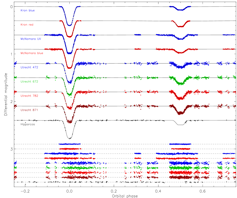
Figure 1: Light curves of YZ Cas from Kron (1939a), Kron (1942), McNamara (1951), de Landtsheer (1983) and Hipparcos (coloured points) compared to the jktebop best fits (black curves). The residuals of the fits are offset from zero to appear at the base of the figure.

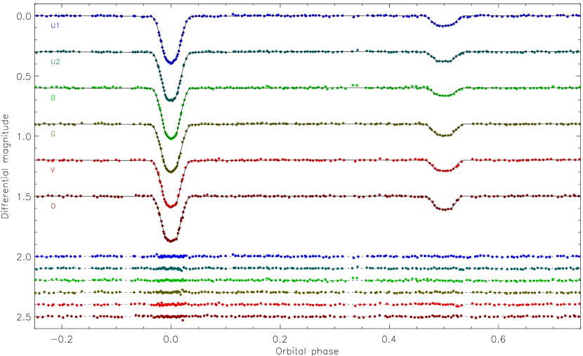
Figure 2: Light curves of YZ Cas from Papoušek (1989) (coloured points) compared to the jktebop best fits (black curves). The residuals of the fits are offset from zero to appear at the base of the figure.

Table 4: Model parameters of the Kron and Utrecht light curves of YZ Cas. The upper part of the table contains fitted parameters and the lower part contains derived parameters. $N_{\rm obs}$ is the number of datapoints in each light curve and the scatter is the rms of the residuals around the best fit.

Parameter	Kron blue		Kron red		Utrecht 472		Utrecht 672		Utrecht 781		Utrecht 871
$J$	0.229 $\pm$	0.006	0.441 $\pm$	0.012	0.255 $\pm$	0.010	0.421 $\pm$	0.014	0.476 $\pm$	0.015	0.503 $\pm$	0.015
$r_{\rm A}+r_{\rm B}$	0.2217 $\pm$	0.0009	0.2178 $\pm$	0.0008	0.2198 $\pm$	0.0029	0.2245 $\pm$	0.0026	0.2235 $\pm$	0.0025	0.2224 $\pm$	0.0025
$k$	0.5286 $\pm$	0.0025	0.5166 $\pm$	0.0017	0.5345 $\pm$	0.0080	0.5310 $\pm$	0.0054	0.5285 $\pm$	0.0051	0.5215 $\pm$	0.0050
$u_{\rm A}$	0.580 $\pm$	0.029	0.361 $\pm$	0.023	0.531 $\pm$	0.092	0.460 $\pm$	0.078	0.359 $\pm$	0.076	0.392 $\pm$	0.073
$u_{\rm B}$	0.65 perturbed		0.50 perturbed		0.65 perturbed		0.50 perturbed		0.40 perturbed		0.35 perturbed
$i$ (°)	88.18 $\pm$	0.10	88.36 $\pm$	0.10	88.18 $\pm$	0.39	87.49 $\pm$	0.25	87.84 $\pm$	0.29	87.87 $\pm$	0.30
$r_{\rm A}$	0.1450 $\pm$	0.0007	0.1436 $\pm$	0.0006	0.1432 $\pm$	0.0021	0.1467 $\pm$	0.0017	0.1462 $\pm$	0.0017	0.1461 $\pm$	0.0017
$r_{\rm B}$	0.0767 $\pm$	0.0003	0.0742 $\pm$	0.0003	0.0766 $\pm$	0.0012	0.0779 $\pm$	0.0011	0.0773 $\pm$	0.0010	0.0762 $\pm$	0.0010
Light ratio	0.0621 $\pm$	0.0006	0.1112 $\pm$	0.0008	0.0692 $\pm$	0.0016	0.1166 $\pm$	0.0017	0.1308 $\pm$	0.0018	0.1387 $\pm$	0.0018
$N_{\rm obs}$	407		565		827		829		835		833
Scatter (mmag)	3.9		5.0		14.7		14.1		14.3		14.6

Table 5: Model parameters of the Papoušek (1989) light curves of YZ Cas. See Table 4 for other details.

Parameter	$U1$		$U2$		$B$		$G$		$V$		$O$
$J$	0.2771 $\pm$	0.0103	0.2584 $\pm$	0.0098	0.2020 $\pm$	0.0095	0.3049 $\pm$	0.0119	0.2921 $\pm$	0.0127	0.3777 $\pm$	0.0139
$r_{\rm A}+r_{\rm B}$	0.2285 $\pm$	0.0030	0.2280 $\pm$	0.0019	0.2222 $\pm$	0.0028	0.2274 $\pm$	0.0022	0.2231 $\pm$	0.0022	0.2192 $\pm$	0.0021
$k$	0.4910 $\pm$	0.0084	0.5260 $\pm$	0.0084	0.5317 $\pm$	0.0091	0.5249 $\pm$	0.0076	0.5126 $\pm$	0.0073	0.5409 $\pm$	0.0059
$u_{\rm A}$	0.892 $\pm$	0.073	0.666 $\pm$	0.085	0.638 $\pm$	0.088	0.639 $\pm$	0.074	0.688 $\pm$	0.071	0.320 $\pm$	0.078
$u_{\rm B}$	0.70 perturbed		0.70 perturbed		0.65 perturbed		0.65 perturbed		0.60 perturbed		0.55 perturbed
$i$ (°)	89.96 $\pm$	0.65	88.18 $\pm$	0.29	88.58 $\pm$	0.41	88.46 $\pm$	0.34	89.11 $\pm$	0.66	88.60 $\pm$	0.36
$r_{\rm A}$	0.1533 $\pm$	0.0026	0.1494 $\pm$	0.0018	0.1451 $\pm$	0.0022	0.1491 $\pm$	0.0018	0.1475 $\pm$	0.0018	0.1423 $\pm$	0.0016
$r_{\rm B}$	0.0752 $\pm$	0.0009	0.0786 $\pm$	0.0010	0.0771 $\pm$	0.0009	0.0783 $\pm$	0.0010	0.0756 $\pm$	0.0009	0.0770 $\pm$	0.0008
Light ratio	0.0724 $\pm$	0.0019	0.0703 $\pm$	0.0020	0.0567 $\pm$	0.0030	0.0835 $\pm$	0.0021	0.0796 $\pm$	0.0031	0.1009 $\pm$	0.0023
$N_{\rm obs}$	175		175		183		164		158		164
Scatter (mmag)	4.7		4.5		5.6		4.9		5.2		5.2

Table 6: Model parameters of the McNamara (1951) and Hipparcos light curves of YZ Cas. The final parameter values, obtained from all fifteen light curves, are given in the last column. See Table 4 for other details.

Parameter	McNamara UV		McNamara blue		Hipparcos		Final values
$J$	0.252 $\pm$	0.010	0.293 $\pm$	0.012	0.321 $\pm$	0.075
$r_{\rm A}+r_{\rm B}$	0.2179 $\pm$	0.0014	0.2201 $\pm$	0.0017	0.2197 $\pm$	0.0053	0.22084 $\pm$	0.00077
$k$	0.5346 $\pm$	0.0054	0.5422 $\pm$	0.0050	0.521 $\pm$	0.032	0.5246 $\pm$	0.0026
$u_{\rm A}$	0.494 $\pm$	0.055	0.354 $\pm$	0.064	0.62 $\pm$	0.29
$u_{\rm B}$	0.65 perturbed		0.65 perturbed		0.60 perturbed
$i$ (°)	88.81 $\pm$	0.26	88.51 $\pm$	0.17	88.49 $\pm$	0.97	88.332 $\pm$	0.066
$r_{\rm A}$	0.1420 $\pm$	0.0011	0.1427 $\pm$	0.0013	0.1445 $\pm$	0.0062	0.14456 $\pm$	0.00056
$r_{\rm B}$	0.0759 $\pm$	0.0006	0.0774 $\pm$	0.0006	0.0752 $\pm$	0.0023	0.07622 $\pm$	0.00033
Light ratio	0.0674 $\pm$	0.0020	0.0764 $\pm$	0.0021	0.088 $\pm$	0.019
$N_{\rm obs}$	894		893		124
Scatter (mmag)	6.6		7.4		7.0

Fig. 3 shows the photometric parameters $r_{\rm A}$, $r_{\rm B}$, $i$, $u_{\rm A}$ and light ratio as a function of wavelength. YZ Cas has sometimes in the past been taken to indicate possible variations of radius with wavelength. Aside from the discrepant results for the bluemost passband (Papoušek $U1$), this figure shows no evidence for a variation with wavelength of $r_{\rm A}$, $r_{\rm B}$ or $i$. The quantity $u_{\rm A}$ has a weak dependence on wavelength and in general higher values than expected theoretically.

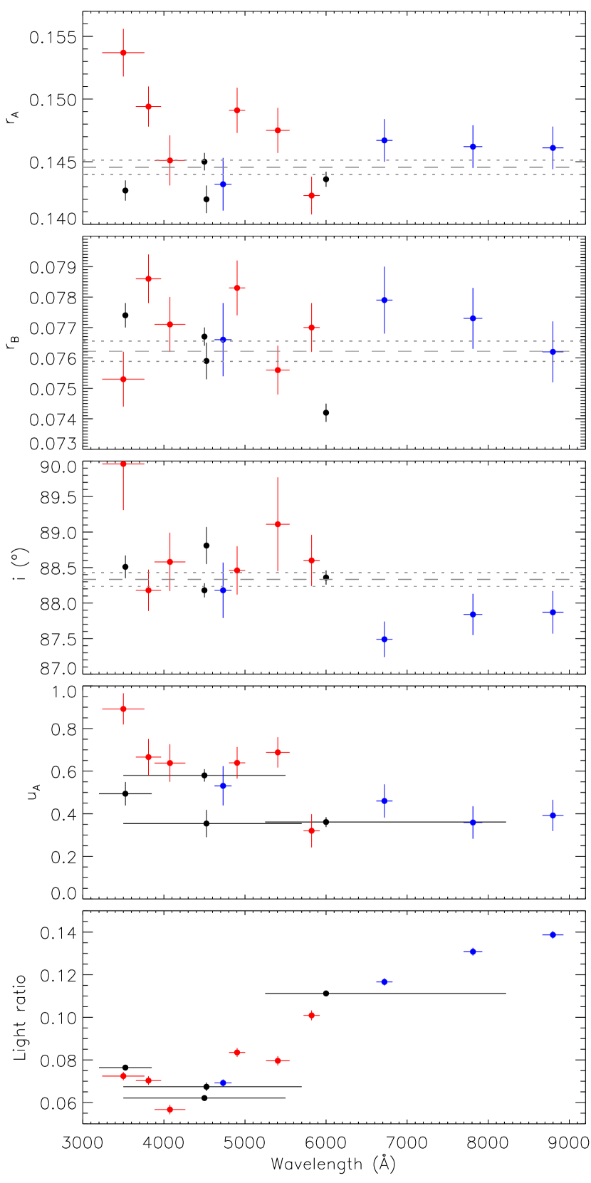
Figure 3: The photometric parameters $r_{\rm A}$, $r_{\rm B}$, $i$, $u_{\rm A}$ and light ratio as a function of wavelength. The Utrecht results are shown using blue lines, the Papoušek (1989) results using red lines, and other results using black lines. The horizontal lines show the widths of the passbands, but the wide passbands are indicated only for the wavelength-dependent quantities in the lower two panels. The dashed horizontal lines show the adopted final values and the dotted horizontal lines indicate the size of the errorbars on these quantities.

For the final photometric parameters we have calculated the weighted mean and its reduced $\chi^{2}$ ($\chi_{\nu}^{\,2}$) of the geometrical quantities (i.e. those which do not depend on wavelength). As expected given the discussion above, we find $\chi_{\nu}^{\,2}>1$ for all quantities. $i$ is least problematic at $\chi_{\nu}^{\,2}=1.4$ and $k$ is the most difficult at $\chi_{\nu}^{\,2}=5.9$. This is a very similar situation to that often found in studies of transiting planetary systems (Southworth, 2008, 2010, 2012). We have therefore multiplied the errorbars of the final weighted-mean values by $\sqrt{\chi_{\nu}^{\,2}}$ to yield reliable errorbars. The large number of available light curves and careful treatment of uncertainties means that our results are robust despite the excess $\chi_{\nu}^{\,2}$ found for some parameters. Final values of the geometrical parameters are given in Table 6 and show that $r_{\rm A}$ and $r_{\rm B}$ have been measured to better than 0.5% precision.

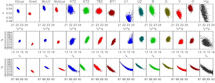
Figure 4: Plots of the variations of best-fit parameters for synthetic datasets generated for the Monte Carlo analysis. From left to right the panels show the light curves in the order they are given in Table 2. For legibility the x-axis labels for the parameters $r_{\rm A}+r_{\rm B}$ and $r_{\rm B}$ are only specified for alternate panels, and the tick values are multiplied by 100 (in effect omitting the leading “0.” in each case). The light curves are colour-coded according to Figs. 1 and 2.

Fig. 4 shows the output from Monte Carlo simulations for each light curve and for the parameters $r_{\rm A}+r_{\rm B}$, $k$, $r_{\rm B}$ and $i$. The points plotted represent best-fit values for each of the synthetic datasets generated for the Monte Carlo simulations. It can be seen that the geometric parameters are actually more precisely defined for the oldest four datasets, and least well-defined for the Hipparcos survey data. The main parameters of the fit, $r_{\rm A}+r_{\rm B}$ and $k$, are very weakly correlated (e.g. correlation coefficient $0.04$ for the Utrecht 672 dataset), whereas the derived parameters $r_{\rm A}$ and $r_{\rm B}$ are more correlated ($0.68$). A strong correlation occurs between $i$ and $r_{\rm B}$ ($-0.89$), as can be seen in the lower panels of Fig. 4.

4.1 Continuum light ratio

The light ratio between the stars is very well determined for YZ Cas, in the passbands for which we have light curves, due to it showing total and annular eclipses. For the spectroscopic analysis in Sect. 6, however, we needed a measurement of the continuum light ratio as a function of wavelength.

We therefore fitted two synthetic spectra from atlas9 model atmospheres (Kurucz, 1979) to the light ratios found in the different passbands. For this we ignored the light curves taken through a wide passband, using only those from de Landtsheer (1983) and Papoušek (1989). The synthetic spectra were used only to fill in the gaps between different passbands, so the choice of their atmospheric parameters was unimportant. Finally, we fitted a second-order polynomial to the light ratio as a function of wavelength (from 4000 to 7000 Å) to give a smooth and continuous proxy to the true light ratio of the system. Star A produces between 86% and 94% of the system light in this wavelength region, being more dominant at bluer wavelengths due to its higher $T_{\rm eff}$ (Fig. 3).

5 Spectroscopic orbit

Table 7: The orbital elements of YZ Cas from SPD. We fixed the orbital period in our analysis to the value found by Lacy (1981).

Parameter	This work		Lacy (1981)
Orbital period $P$ (d)	4.4672235		4.4672235
Orbital eccentricity $e$	0 (fixed)		0.0 $\pm$	0.003
Velocity amplitude $K_{\rm A}$ ( km s-1)	73.05 $\pm$	0.19	73.35 $\pm$	0.35
Velocity amplitude $K_{\rm B}$ ( km s-1)	124.78 $\pm$	0.27	125.7 $\pm$	0.5
Mass ratio $q$	0.585 $\pm$	0.002	0.583 $\pm$	0.008

The small light contribution of star B makes the measurement of its orbital motion and atmospheric parameters relatively challenging, even from échelle spectra. We have therefore used the spectral disentangling (SPD) approach for our spectroscopic analysis. SPD of time-series spectra of binary star systems (Simon & Sturm, 1994) is a powerful technique which enables the determination of the optimal set of the orbital parameters of a binary system, and the individual spectra of the components, simultaneously and self-consistently. A discussion of SPD and its practical applications can be found in reviews by Pavlovski & Hensberge (2010) and Pavlovski & Southworth (2012).

As YZ Cas is a dEB, we have followed the analysis approach described in detail by Hensberge et al. (2000). SPD was performed with the FDBinary code (Ilijić et al., 2004) which implements the Fourier approach of Hadrava (1995). Since no spectra were obtained during totality in eclipse, there is an ambiguity in the determination of the continuum level. Therefore, SPD was performed in pure separation mode and renormalisation of disentangled spectra of the individual components to their continua was done with the light ratio derived from the light curves in Section 4.1 (Pavlovski & Southworth, 2012). Since FDBinary is based on discrete Fourier transforms there is no limitation on the length or resolution of the spectra to be analysed, so far as the basic prescriptions for Fourier disentangling are fulfilled.

There is no indication from photometry (Sections 3 and 4) or previous spectroscopy (Koch et al., 1965; Lacy, 1981) that the orbit is eccentric. We therefore fixed $e$ to zero in our analysis, and fitted only for the velocity amplitudes of the two stars ($K_{\rm A}$ and $K_{\rm B}$). Spectral regions containing Balmer lines were avoided in the optimisation of $K_{\rm A}$ and $K_{\rm B}$, as SPD is very sensitive to minor imperfections in continuum placement over these extremely broad lines. The large wavelength interval covered by our échelle spectra means that there is plenty of spectrum with a well-defined continuum and containing only metallic lines. SPD was performed and $K_{\rm A}$ and $K_{\rm B}$ calculated for a number of spectral intervals of widths ranging from 50 Å to 100 Å. The quality of the normalisation and merging of the spectra is reflected in very small standard deviations of the values of $K_{\rm A}$ ($\pm$0.03 km s^-1) and $K_{\rm B}$ ($\pm$0.04 km s^-1).

A second estimate of the uncertainties in $K_{\rm A}$ and $K_{\rm B}$ can be obtained using other techniques for least-squares analysis such as bootstrap resampling, but such analysis can require a lot of computation time. We have therefore performed a jackknife test where a set of solutions are calculated, each one ignoring a single observed spectrum. We have previously found reasonable and realistic results using this approach for the dEB AS Cam (Pavlovski et al., 2011). This was done for seven of the spectral regions, with the result that the jackknife-derived uncertainties ($\sim$0.2 km s^-1 and $\sim$0.3 km s^-1) are roughly one order of magnitude greater than the standard deviation in $K_{\rm A}$ and $K_{\rm B}$ for these spectral regions ($\pm$0.04 km s^-1 and $\pm$0.05 km s^-1). We accept the jackknife uncertainties as our final errorbars (Table 7); they correspond to measurement uncertainties of 0.5% in the masses of the two stars. This is a realistic result for 42 high-quality échelle spectra of a dEB containing slowly rotating stars in a circular orbit.

6 Atmospheric parameters

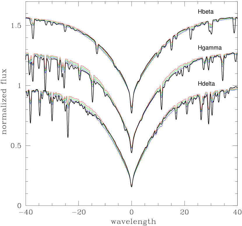
Figure 5: Determination of the $T_{\rm eff}$ of YZ Cas A from its Balmer line profile. The renormalised disentangled profiles are shown by thin black lines, and theoretical lines profiles for $T_{\rm eff}$s of 9800, 9600 and 9400 K are shown by red, blue and green lines. From top to bottom the profiles are of H$\beta$, H$\gamma$ and H$\delta$. The surface gravity is fixed from the light and RV curve analyses.

The complexity of spectra of close binary systems due to their composite nature and continuously varying Doppler shifts makes the extraction of atmospheric parameters non-trivial. The SPD technique is an important aid to such studies, as it allows the derivation of the individual spectra of the two stars without needing template spectra for guidance. These separated spectra can then be analysed as if they were observed spectra of single stars, allowing the determination of the $T_{\rm eff}$s and chemical composition of the two components of the binary system. These numbers are in turn important for the use of dEBs as distance indicators (e.g. Hensberge et al., 2000; North et al., 2010) and as critical tests of stellar evolutionary theory (e.g. Pavlovski et al., 2009; Brogaard et al., 2011).

The first uses of SPD to estimate $T_{\rm eff}$s from disentangled individual component spectra were made for the close binaries DH Cep by Sturm & Simon (1994) and Y Cyg by Simon et al. (1994). These authors also estimated helium abundances for the components in the systems. On these grounds Hensberge et al. (2000) constructed a self-consistent complementary approach in the analysis of close binary stars. In a detailed study of the high-mass double-lined dEB V578 Mon, Hensberge et al. were able to determine the basic physical properties more accurately than possible using ‘standard’ techniques. In a follow-up study Pavlovski & Hensberge (2005) presented the first abundance analysis using the broad wavelength range available in disentangled échelle spectra.

In this work we follow the approach of Hensberge et al. (2000). The disentangled spectra have to be normalised to their intrinsic continua as this cannot be done by SPD. SPD essentially attibutes spectral features to the individual stars according to their orbital motion, and this is not possible for continuum flux unless spectra were obtained during eclipse. The light factor (LFs) which give the continuum level of each star can be obtained either from the light curves (using the light ratios from the best-fitting eclipse model) or by constrained fitting of the Balmer lines of both components simultaneously (Tamajo et al., 2011).

6.1 Effective temperature and microturbulence

We proceeded to estimate the $T_{\rm eff}$ of star A by fitting its Balmer line profiles and then fine-tuning the value using the ionisation balance of the many Fe lines in the spectrum. The Balmer lines in A-type stars are sensitive both to $T_{\rm eff}$ and surface gravity, $\log g$. In the case of YZ Cas, this degeneracy can be easily sidestepped since our analysis of the light and RV curves results in a measurement of $\log g$ for both stars to an accuracy of better than 0.01 dex; this is an intrinsic advantage for spectroscopic analysis of EBs.

Spectral disentangling was performed on three spectral intervals of 150–250 Å width, centred on H$\beta$, H$\gamma$ and H$\delta$. In the SPD of early-type stars these are the most difficult and uncertain spectral regions since Doppler shifts due to orbital motion are much smaller than the intrinsic widths of the Balmer lines. In order to minimise systematic errors in the normalisation and merging of échelle orders containing broad Balmer lines we developed a semi-automatic procedure. A high-order polynomial fit of the blaze function was calculated in adjacent well-defined (‘cleaner’) échelle orders. Then the blaze function was constructed for échelle orders containing broad Balmer lines by interpolation and scaling between adjacent orders. We used the light ratio measured from the photometric analysis (Sect. 4.1) to normalise the disentangled spectra to the intrinsic continuum of each star. Since the disentangled (separated) spectra of the components have to be corrected for the dilution effect, in this particular case by factors of about 1.08 for star A, and 14.3 for star B, any imperfections in the continuum placement or the determination of the light ratio would be scaled up by the same amount. Because of the large light ratio between the components, as well as their atmopsheric properties, in this work the effective temperature was determined from Balmer lines only for star A. It was then used for deriving the $T_{\rm eff}$ of star B through the photometric analysis, and as a starting point in determination of the $T_{\rm eff}$ of star A through detailed spectroscopic analysis.

A grid of local thermodynamic equilibrium (LTE) synthetic spectra was calculated using the uclsyn code (Smith, 1992; Smalley et al., 2001) and atlas9 model atmospheres for solar metallicity $\left[\frac{\rm M}{\rm H}\right]=0$. The grid covers $T_{\rm eff}$s from 8400 K to 10 400 K in steps of 200 K, for the known surface gravity of star A ($\log g=3.988$). The $T_{\rm eff}$ of star A was determined by minimising the difference between the reconstructed disentangled spectra and the synthetic spectra in the spectral ranges of H$\delta$ (4070–4170 Å), H$\gamma$ (4290–4370 Å) and H$\beta$ (4800–4900 Å). Minimisation was performed separately on the blue and red wings. Metallic lines contaminating the Balmer profiles were masked out during this process. Minimisation from these six wings of Balmer lines gave $T_{\rm eff}=9670\pm 140$ K for star A, where the errorbar is the 1$\sigma$ error. In Fig. 5 we show the quality of fit to the observed (disentangled) spectra of the Balmer lines by the synthetic spectra.

In the spectra of the components several species appear in two or even three ionization stages, e.g. Si for star A. The most numerous lines in the spectra of both components are Fe i and Fe ii lines, and they are well suited to the determination of both $T_{\rm eff}$ and microturbulent velocity ($v_{\rm turb}$). $T_{\rm eff}$ was determined from Fe i and Fe ii lines under the condition that abundances should not depend on ionisation state or excitation potential (Gray, 2008). We determined $v_{\rm turb}$ by requiring the Fe abundance to be independent of equivalent width (EW) (Magain, 1984).

The measurements of EWs were obtained by direct integration of the line profiles and abundances for Fe i and Fe ii calculated using uclsyn. We have followed the critical selection of Fe i and Fe ii lines from Qiu et al. (2001) in deriving $T_{\rm eff}$ and $v_{\rm turb}$, but all identified Fe  lines were measured. The lines were selected on the basis of the reliability of their atomic data, mostly gf values, and their strength. We agree with Qiu et al. (2001) that including all lines, most of which are weak lines with EW $<5$ mÅ, results in a larger scatter and less reliable abundances. In total we have 51 Fe i and 30 Fe ii reliable lines for star A (see Table 8), with EWs ranging from 5 to 100 mÅ. For the cooler star B there are many more Fe lines, 216 Fe i and 24 Fe ii, and these have EWs of 5–70 mÅ. All Fe lines detected were checked against new entries for gf values in the vald line lists (Kupka et al., 2000, and references therein).

For star A we found $T_{\rm eff}=9520\pm 120$ K, in acceptable agreement with the value from fitting the Balmer lines, and $v_{\rm turb}=3.8\pm 0.1$ km s^-1. In the case of star B, we estimated a preliminary $T_{\rm eff}$ from its colour indices because its Balmer lines are much weaker. We refined the value using the ionisation balance of Fe, finding $T_{\rm eff}=6880\pm 240$ K and $v_{\rm turb}=1.7\pm 0.1$ km s^-1. The observed spectra are quite sensitive to $v_{\rm turb}$ so we have been able to constrain the values well. The derived value for star A is typical for Am stars (e.g. Landstreet et al., 2009) whilst the value for star B fits the trend found for stars of similar $T_{\rm eff}$ (e.g. Bruntt et al., 2010; Doyle et al., 2013).

de Landtsheer & Mulder (1983) estimated the $T_{\rm eff}$ of star A from an IUE low-resolution calibrated spectrum, in a determination also involving the distance and line-of-sight interstellar extinction for YZ Cas. The authors concluded that $T_{\rm eff}=10\,600\pm 400$ K, arguing against the value of $9000$ K resulting from visual spectral classification (Hill et al., 1975). Ribas et al. (2000) used intermediate-band photometry and grids of spectra from model atmospheres to revise the $T_{\rm eff}$ scale using a sample of dEBs. They found $T_{\rm eff}=9100\pm 300$ K for star A and $T_{\rm eff}=6600\pm 250$ K for star B. Our spectroscopic results, based both on Balmer line profiles and Fe ionisation balance, corroborate their estimates to within 1$\sigma$.

6.2 Abundances

Table 8: Measured chemical abundances in the photospheres of the component stars of YZ Cas, derived in the LTE approximation. $N$ is the number of lines used for each element.

Ion	YZ Cas A					YZ Cas B
	$N$	$\log\epsilon{\rm(X)}$		[X/H]		$N$	$\log\epsilon{\rm(X)}$		[X/H]
C	55	8.85 $\pm$	0.10	0.36 $\pm$	0.11	29	8.49 $\pm$	0.06	0.06 $\pm$	0.08
O	25	9.03 $\pm$	0.08	0.34 $\pm$	0.09	10	8.89 $\pm$	0.13	0.20 $\pm$	0.14
Na	5	6.99 $\pm$	0.08	0.68 $\pm$	0.09	8	6.34 $\pm$	0.08	0.10 $\pm$	0.10
Mg	19	7.91 $\pm$	0.09	0.26 $\pm$	0.10	14	7.52 $\pm$	0.14	$-$0.08 $\pm$	0.15
Al	2	7.26 $\pm$	0.09	0.73 $\pm$	0.09
Si	63	7.89 $\pm$	0.08	0.31 $\pm$	0.09	46	7.48 $\pm$	0.05	$-$0.03 $\pm$	0.07
S	22	7.83 $\pm$	0.12	0.65 $\pm$	0.12	13	7.26 $\pm$	0.04	0.14 $\pm$	0.05
Ca	29	6.66 $\pm$	0.11	0.27 $\pm$	0.12	25	6.37 $\pm$	0.11	0.03 $\pm$	0.12
Sc	13	3.01 $\pm$	0.11	$-$0.19 $\pm$	0.12	10	3.11 $\pm$	0.07	$-$0.04 $\pm$	0.08
Ti	70	5.37 $\pm$	0.11	0.34 $\pm$	0.12	120	4.97 $\pm$	0.12	0.02 $\pm$	0.13
V	9	4.45 $\pm$	0.09	0.47 $\pm$	0.12	13	4.10 $\pm$	0.13	0.17 $\pm$	0.15
Cr	71	6.24 $\pm$	0.09	0.53 $\pm$	0.10	127	5.67 $\pm$	0.11	0.03 $\pm$	0.12
Mn	22	5.91 $\pm$	0.12	0.39 $\pm$	0.11	23	5.40 $\pm$	0.10	$-$0.03 $\pm$	0.11
Fe	81	8.12 $\pm$	0.10	0.54 $\pm$	0.11	240	7.51 $\pm$	0.10	0.01 $\pm$	0.11
Co						44	5.01 $\pm$	0.13	0.02 $\pm$	0.15
Ni	8	6.96 $\pm$	0.09	0.67 $\pm$	0.10	109	6.25 $\pm$	0.11	0.03 $\pm$	0.12
Cu	1	4.70 $\pm$	0.13	0.43 $\pm$	0.14	9	4.19 $\pm$	0.11	0.00 $\pm$	0.12
Zn	1	5.80 $\pm$	0.13	1.17 $\pm$	0.14	2	4.60 $\pm$	0.17	0.04 $\pm$	0.18
Y	6	3.25 $\pm$	0.11	0.96 $\pm$	0.12	14	2.26 $\pm$	0.08	0.05 $\pm$	0.09
Zr	5	3.64 $\pm$	0.14	0.99 $\pm$	0.16	8	2.58 $\pm$	0.12	0.00 $\pm$	0.13
Ba	2	3.43 $\pm$	0.15	1.15 $\pm$	0.18	2	2.19 $\pm$	0.12	0.01 $\pm$	0.15
La						19	1.29 $\pm$	0.10	0.19 $\pm$	0.11
Ce						26	1.58 $\pm$	0.11	0.00 $\pm$	0.12
Pr						4	0.72 $\pm$	0.12	0.00 $\pm$	0.13
Nd						31	1.56 $\pm$	0.10	0.14 $\pm$	0.11
Sm						2	1.08 $\pm$	0.17	0.12 $\pm$	0.17

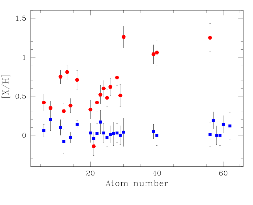
Figure 6: Comparison between abundances derived for star A (red filled circles) and star B (blue filled squares).

For stars with $T_{\rm eff}$s similar to those of the components of YZ Cas, a large number of spectral lines arise from neutral and singly ionised species. The number of good lines for abundance determination is, however, decreased due to the rotation of the component stars. We selected good lines based on the quality of their atomic data and the amount of blending with other lines.

We used uclsyn to measure EWs and calculate the abundances. Table 8 contains the derived abundances for all elements identified in the spectrum of either star, in two forms. Firstly, the number density $\epsilon$ is given on a scale where $\log\epsilon{\rm(H)}=12.0$. Secondly, the value for element X is converted into logarithmic abundance versus the Sun ([X/H]) using the standard solar abundances from Asplund et al. (2009), the most recent critical evaluation of the solar abundances. The errorbars on these quantities are the r.m.s. errors of the results for individual lines, so are indicative of the number and quality of the lines used rather than the true uncertainties. Additional contributions to the uncertainties arise from the quality of the atomic data, the quality of the spectra and their normalisation, and uncertainties in the measured $T_{\rm eff}$, $\log g$ and $v_{\rm turb}$ values. The spectra are of high quality and their normalisation is well-defined away from the Balmer lines, so these should not give rise to significant systematic errors. Similarly, the atmospheric parameters are measured to high precision so will not cause much uncertainty.

The abundances in Table 8 are visualised in Fig. 6. We find that the chemical abundances for star B are close to solar; a calculation of the metallicity from the abundances listed in Table 8 for star B and replacing missing elements with abundances given by Asplund et al. (2009) returns a value of $Z=0.0170\pm 0.024$ (where $Z$ is the mass fraction of metals) which is slightly more than 1$\sigma$ away from the solar value of $Z=0.0134$ derived in Asplund et al. (2009). These values should be appropriate for the bulk chemical composition of the system as a whole because the photosphere is expected to represent the internal composition for a 6880 K dwarf star. The abundances for star A are all significantly super-solar except for Sc, confirming the Am nature of this star. Zn, Y, Zr and Ba are all overabundant by 1 dex relative to solar. We have not been able to measure the abundances of any rare-earth elements, even though a strong over-abundance of these is a hallmark of the Am phenomenon (Wolff, 1983).

We calculated a provisional set of abundances for star A using model atmospheres of solar abundance rather than abundances tuned to the true metallicity of the star. For our final abundance measurements (Table 8), we used model atmospheres with scaled-solar metallicity and a metal abundance of [X/H] $=$ 0.5. The use of scaled-solar model atmospheres should be sufficient for our work because the blanketing effect on the atmospheric structure is mostly due to iron-group elements. Smalley (1993) has shown the effect on the derived abundances to be small: a few hundreths of a dex in abundance and probably no more than 100 K in $T_{\rm eff}$. We found that the use of model atmospheres with [X/H] $=$ 0.5 rather than solar abundance had the effect of increasing the derived abundances for all elements by between 0.05 and 0.10 dex, with the exception of oxygen for which the measured abundance increased by 0.003 dex, only.

There exists one previous abundance study of YZ Cas, by de Landtsheer & Mulder (1983). These authors derived the atmospheric properties and the abundances of six elements from IUE high-resolution spectra. They adopted a higher $T_{\rm eff}$ (10 600 K) and measured a higher $v_{\rm turb}$ ($5.8\pm 1.7$ km s^-1) than we find, and this is probably why they derived exceptionally high abundance values (from 0.80 dex for Fe to 3.4 dex for Co relative to solar). We do not confirm these overabundances for five of the six chemicals (Si, Cr, Mn, Fe, Ni). We did not obtain an abundance for the sixth, Co, but the value from de Landtsheer & Mulder (1983) is almost certainly also wrong.

6.3 Rotational velocity

The disentangled spectra of YZ Cas have S/N values of about 1500 and 200 for star A and star B, respectively, and are rich in information. We first measured the instrumental broadening profile using both ThAr emission lines and and telluric absorption lines, finding FWHM $=$ 0.13 Å. Despite both stars having only moderate rotational velocities, the lines in their spectra are strongly overlapping. We therefore measured $v\sin i$ by line-profile fitting of complex blends using the uclsyn code.

In each disentangled spectrum several spectral regions were selected containing lines with good atomic data. Line-profile fitting then yielded $v_{\rm A}\sin i=29.2$ km s^-1 and $v_{\rm B}\sin i=15.0$ km s^-1. The formal errors on these determinations are $\pm$0.1 km s^-1 and $\pm$0.3 km s^-1, respectively. Additional contributions to these uncertainties come from the instrumental broadening, its variation with wavelength, continuum normalisation, microturbulence and macroturbulence. We therefore adopt larger errorbars of $\pm$0.5 km s^-1 for both $v\sin i$ measurements.

If both components show synchronous rotation the ratio of their velocities should equal the ratio of their radii. We find $v_{\rm A}\sin i/v_{\rm B}\sin i=0.514\pm 0.019$ and $k=0.5246\pm 0.0026$, so these values are consistent to within 0.5$\sigma$. This matches our expectation that the components should be rotating synchronously with the orbital motion.

7 The physical properties and distance of YZ Cassiopeiae

Table 9: The physical properties of the YZ Cas system.

Parameter	Star A		Star B
Orbital separation ($\,{\rm R}_{\odot}$)	$17.468\pm 0.029$
Mass ($\,{\rm M}_{\odot}$)	2.263 $\pm$	0.012	1.325 $\pm$	0.007
Radius ($\,{\rm R}_{\odot}$)	2.525 $\pm$	0.011	1.331 $\pm$	0.006
$\log g$ [cm s-2]	3.988 $\pm$	0.004	4.311 $\pm$	0.004
$V_{\rm synch}$ ( km s-1)	28.61 $\pm$	0.12	15.08 $\pm$	0.07
$v\sin i$ ( km s-1)	29.2 $\pm$	0.5	15.0 $\pm$	0.5
$T_{\rm eff}$(K)	9520 $\pm$	120	6880 $\pm$	240
$\log(L/\,{\rm L}_{\odot})$ 1	1.672 $\pm$	0.022	0.552 $\pm$	0.061
$M_{\rm bol}$ 1	0.57 $\pm$	0.06	3.37 $\pm$	0.15
Distance (pc)	$103.8\pm 1.3$

¹ Calculated assuming $\,{\rm L}_{\odot}=3.844$$\times$10²⁶ W (Bahcall et al., 1995) and $M_{\rm bol}\sun=4.75$ (Zombeck, 1990).

Using the photometric and spectroscopic results from Sections 4 and  5, we have calculated the physical properties of the YZ Cas system (Table 9). This was done using the jktabsdim code (Southworth et al., 2005a), which propagates uncertainties via a perturbation analysis. We adopted the physical constants tabulated by Southworth (2011). The masses and radii are measured to precisions of 0.5%, representing a useful improvement over previous analyses. The high precision of these determinations is due to several circumstances. Firstly, we had access to extensive observational data: 15 published light curves plus 42 new high-quality échelle spectra. Secondly, the intrinsic character of the system makes it well-suited to detailed analysis. The total eclipses mean the light curve solutions are very well-defined, and the slow rotation and large number of spectral lines means the orbital velocities of the two components are measurable to high precision. Compared to Lacy (1981), we find very similar radii but masses smaller by 2–3$\sigma$.

We have also measured the atmospheric parameters of both stars to high precision. Our new $T_{\rm eff}$ measurements are precise and support previous optical rather than UV determinations. The rotational velocities of both stars are consistent with synchronocity, as expected from the timescales for rotational synchronisation (see Zahn, 1975, 1977).

From the known masses and radii and the $T_{\rm eff}$s obtained in Sect. 6 we have calculated the luminosities (expressed logarithmically with respect to the Sun in Table 9) and absolute bolometric magnitudes of the two stars. From these we have measured the distance to the system using empirical surface brightness relations (see Southworth et al. 2005a and Kervella et al. 2004) and by the usual method involving bolometric corrections (e.g. Southworth et al., 2005b). For this process we adopted apparent magnitudes in the $B$ and $V$ bands from Høg et al. (1997) and in the $JHK_{s}$ bands from Skrutskie et al. (2006). Tabulated bolometric corrections were taken from Bessell et al. (1998) and Girardi et al. (2002). All distance measurements agree well, and we take the $K_{s}$-band surface-brightness-based distance of $103.8\pm 1.3$ pc as our final value.

The good agreement between the optical ($BV$) and IR ($JHK_{s}$) distance measurements argues against the presence of significant interstellar absorption; by requiring consonant distances we find an upper limit of only $E(B-V)=0.03$ mag (3$\sigma$). We have also interpreted the light ratio derived from the Papoušek (1989) $V$ light curve as a light ratio in the Johnson $V$ band to obtain a separate distance estimate for the two stars. These agree to within their errorbars, so the $T_{\rm eff}$s and radii in Table 9 pass this consistency check.

Both stars in YZ Cas are situated outside the $\delta$ Sct instability strip (Dupret et al., 2005; Uytterhoeven et al., 2011): star A is hotter than the blue edge of the fundamental radial mode, and star B is cooler than its red edge. With a $T_{\rm eff}$ of 9520 K, star A is among the hottest of the Am stars.

8 Comparison with theoretical models

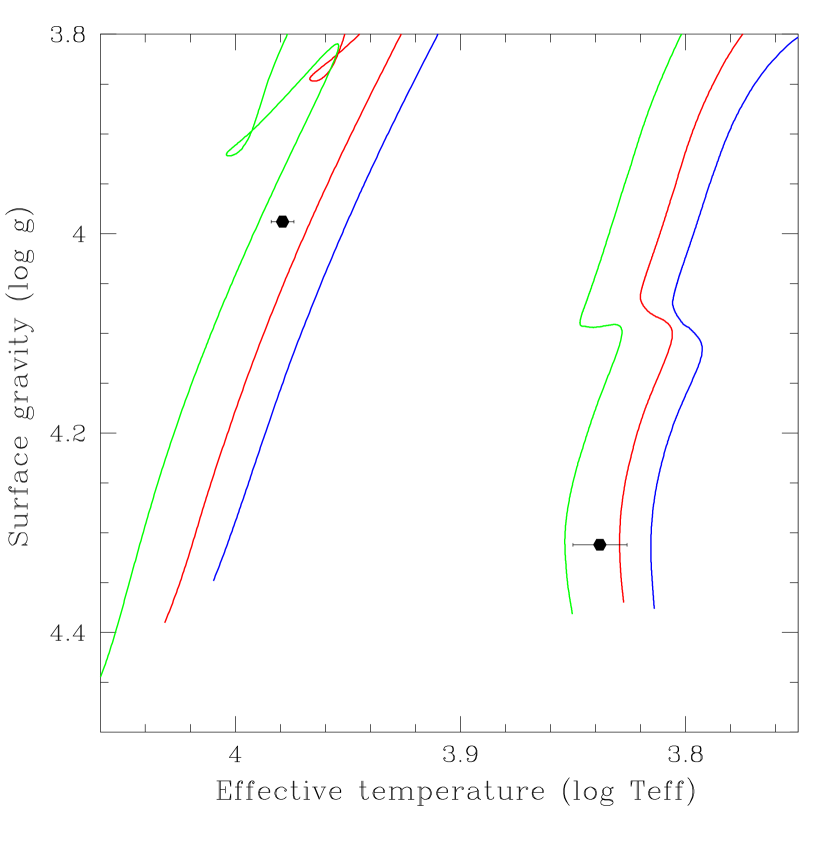
Figure 7: The locations of the components of YZ Cas in the $\log T_{\rm eff}$ versus $\log g$ plane. The Geneva evolutionary tracks (Mowlavi et al., 2012) for their masses are plotted for the metallicity values $Z=0.006$ (green lines), 0.010 (red lines) and 0.014 (blue lines).

Considerable attention has been devoted to the metallicity of the component stars of YZ Cas. The relatively large difference in their masses means they could be a stringent test of the stellar evolutionary models (Lastennet & Valls-Gabaud, 2002). These authors found a problem in the discrepancy in metallicity estimated from matching the physical properties of the system to the predictions of theoretical stellar models ($Z=0.015$), and the metallicity derived for star A from UV spectroscopy ($Z=0.036\pm 0.005$; de Landtsheer & Mulder 1983). Lastennet et al. (2001) challenged the UV metallicity determination on the basis that photometric methods do not indicate a high $Z$ and are in fact compatible with solar metallicity.

Our detailed abundance analysis based on optical échelle spectra has revealed the photospheric chemical composition of both stars. Star A shows a high metallicity which cannot be taken as an indication of its internal composition. Star B, however, shows a solar metallicity which should be representative of its bulk metal abundance.

We have compared the masses, radii and $T_{\rm eff}$s of the components of YZ Cas to tabulated predictions from several sets of theoretical stellar evolutionary models. An immediate results is that the best fit to the observed properties is found for a subsolar metal abundance, whereas a solar metallicity results in predicted $T_{\rm eff}$s which are too small to match the observed values. We also were able to infer a precise age, $\tau$, for the system. The Teramo models (Pietrinferni et al., 2004) give a good fit for $Z=0.010$ and $\tau=490$ Myr, with a slight preference for models with core overshooting over canonical models. The VRSS models (VandenBerg et al., 2006) agree very well with the measured properties for $Z=0.010$ and $\tau=545$ Myr, with an acceptable fit also being found for $Z=0.0125$ and $\tau=530$ Myr. The PARSEC models (Bressan et al., 2012) for $Z=0.010$ and $\tau=545$ Myr are almost identical to the VRSS ones, so also fit well. Finally, an investigation of the Y² models (Demarque et al., 2004) resulted in a good fit for $Z=0.01$ and $\tau=550$ Myr, where a higher $Z$ causes the predicted $T_{\rm eff}$s to become too low and a lower $Z$ underpredicts the radius of star B.

In Fig. 7 we show an alternative approach where evolutionary tracks interpolated to the specific masses of the two stars are plotted in the $\log T_{\rm eff}$ versus $\log g$ diagram for three metallicities. The models used are the most recent versions from the Geneva group (Mowlavi et al., 2012), which have modest convective core overshooting and do not account for stellar rotation. We found the best-fitting metallicities and ages to be $Z=0.008\pm 0.001$ and 420 Myr for star Am and $Z=0.009\pm 0.002$ and 670 Myr for star B. This corroborates our inferences from the four sets of models discussed above.

We therefore find that the physical properties of both stars match the predictions of theoretical models for a metallicity of $Z=0.009\pm 0.003$ and an age of 400–700 Myr. This is troubling because the photospheric abundances we find for star B show it to have an approximately solar chemical composition. We coclude that either the theoretical models are incorrect or the photospheric abundances of star B do not represent its bulk chemical composition.

9 Conclusions

We have presented a detailed analysis of the dEB YZ Cas based on 15 published light curves and 42 new high-quality échelle spectra. The principal attraction of this object is that it contains two quite different stars: one an A-type metallic-lined star and the other a smaller and less massive F2 dwarf. We were therefore able to investigate the Am nature of star A using the chemically normal star B as a reference.

We have measured the masses and radii of both component to a precision of 0.5%, due to the large amount of observational material as well as the co-operative nature of the system. The time-resolved spectra were analysed using spectral disentangling, allowing us to derive the individual spectra of the two stars as well as their velocity amplitudes. From the separated spectra we obtained the atmospheric parameters ($T_{\rm eff}$ and $v_{\rm turb}$) and photospheric chemical compositions of both stars.

Star A shows clear signs of the Am phenomenon: enhanced metals, depleted Sc, and over-abundances of Zn, Y, Zr and Ba by 1 dex. By contrast, star B shows normal chemical abundances which are consistent with a solar or slightly super-solar chemical composition. Whilst the Am phenomenon is a ‘surface disease’, the abundances of star B should represent the bulk chemical composition of both stars. It is therefore surprising that theoretical stellar evolutionary models require a significantly sub-solar metallicity to reproduce the properties of the YZ Cas system. Our results cannot differentiate between the possibilities that the model predictions are wrong and that the photospheric abundances of star B do not represent the true chemical composition of either star.

The Am stars are defined phenomenologically: in classification-resolution spectra the Ca K line is appropriate for an early-A spectral type and metallic lines point to a late-A to F type, whilst the hydrogen Balmer lines are intermediate (Roman et al., 1948). With the widespread use of higher-resolution spectra a new definition of the Am phenomenon has evolved. Conti (1970) defined it as an apparent surface underabundance of Ca and/or Sc, and/or an apparent overabundance of Fe-group and heavier elements. Modern spectroscopic studies have revealed much variety in observed abundance patterns, and difficulties exist in delineating the border between normal and chemically peculiar A stars. Interesting discussions of the Am phenomenon in can be found in Adelman & Unsuree (2007) and Murphy et al. (2012). While Am stars were long considered to have quiet atmospheres that were therefore not pulsating, high-precision photometry from both ground-based (SuperWASP) and space-based (Kepler) surveys have yielded the detection of more than 200 A and F dwarfs with Am characteristics and detectable pulsations (Smalley et al., 2011; Balona et al., 2011). Important constraints of the origin of the Am phenomenon are also provided by their rotation and binarity (Fossati et al., 2008; Stateva et al., 2012).

Our work on YZ Cas has yielded precise measurements of the mass, radius and $T_{\rm eff}$ of an Am star, plus the abundances of 26 elements in its photosphere. Its F2 V companion has a solar chemical composition which should reflect the internal composition of both stars. Theoretical models cannot reproduce the physical properties of the stars for this composition. Further work is needed to understand the nature of this discrepancy and to model the processes occurrent in the atmospheres of Am stars.

References

- Abt (1961) Abt, H. A., 1961, ApJS, 6, 37
- Abt (1965) Abt, H. A., 1965, ApJS, 11, 429
- Abt & Levy (1985) Abt, H. A., Levy, S. G., 1985, ApJS, 59, 229
- Adelman & Unsuree (2007) Adelman, S. J., Unsuree, N., 2007, Baltic Astronomy, 16, 183
- Andersen (1991) Andersen, J., 1991, A&ARv, 3, 91
- Argelander (1903) Argelander, F., 1903, Bonner Durchmusterung des nordlichen Himmels, Marcus and Weber’s Verlag, Bonn
- Asplund et al. (2009) Asplund, M., Grevesse, N., Sauval, A. J., Scott, P., 2009, ARA&A, 47, 481
- Bahcall et al. (1995) Bahcall, J. N., Pinsonneault, M. H., Wasserburg, G. J., 1995, Reviews of Modern Physics, 67, 781
- Balona et al. (2011) Balona, L. A., et al., 2011, MNRAS, 414, 792
- Bessell (2000) Bessell, M. S., 2000, PASP, 112, 961
- Bessell et al. (1998) Bessell, M. S., Castelli, F., Plez, B., 1998, A&A, 333, 231
- Bonanos et al. (2006) Bonanos, A. Z., et al., 2006, ApJ, 652, 313
- Brát et al. (2008) Brát, L., et al., 2008, Open European Journal on Variable Stars, 94
- Brelstaff (1994) Brelstaff, T., 1994, Br. Astron. Assoc., Var. Star Sect. Circ., 81, 4
- Bressan et al. (2012) Bressan, A., Marigo, P., Girardi, L., Salasnich, B., Dal Cero, C., Rubele, S., Nanni, A., 2012, MNRAS, 427, 127
- Brogaard et al. (2011) Brogaard, K., Bruntt, H., Grundahl, F., Clausen, J. V., Frandsen, S., Vandenberg, D. A., Bedin, L. R., 2011, A&A, 525, A2
- Bruntt et al. (2010) Bruntt, H., et al., 2010, MNRAS, 405, 1907
- Budaj (1996) Budaj, J., 1996, A&A, 313, 523
- Budaj (1997) Budaj, J., 1997, A&A, 326, 655
- Cannon & Pickering (1918) Cannon, A. J., Pickering, E. C., 1918, Annals of Harvard College Observatory, 91, 1
- Carquillat & Prieur (2007) Carquillat, J., Prieur, J., 2007, MNRAS, 380, 1064
- Claret (2000) Claret, A., 2000, A&A, 363, 1081
- Claret (2004) Claret, A., 2004, A&A, 428, 1001
- Claret & Hauschildt (2003) Claret, A., Hauschildt, P. H., 2003, A&A, 412, 241
- Clausen et al. (2008) Clausen, J. V., Torres, G., Bruntt, H., Andersen, J., Nordström, B., Stefanik, R. P., Latham, D. W., Southworth, J., 2008, A&A, 487, 1095
- Conti (1970) Conti, P. S., 1970, PASP, 82, 781
- Cutri et al. (2003) Cutri, R. M., et al., 2003, 2MASS All Sky Catalogue of point sources., The IRSA 2MASS All-Sky Point Source Catalogue, NASA/IPAC Infrared Science Archive
- de Landtsheer (1983) de Landtsheer, A. C., 1983, A&AS, 53, 161
- de Landtsheer & De Greve (1984) de Landtsheer, A. C., De Greve, J. P., 1984, A&A, 135, 397