Accuracy of Algebraic Fourier Reconstruction for Shifts of Several Signals

Abstract

We consider the problem of “algebraic reconstruction” of linear combinations of shifts of several known signals $f_{1},\ldots,f_{k}$ from the Fourier samples. Following [5], for each $j=1,\ldots,k$ we choose sampling set $S_{j}$ to be a subset of the common set of zeroes of the Fourier transforms ${\cal F}(f_{\ell}),\ \ell\neq j$, on which ${\cal F}(f_{j})\neq 0$. It was shown in [5] that in this way the reconstruction system is “decoupled” into $k$ separate systems, each including only one of the signals $f_{j}$. The resulting systems are of a “generalized Prony” form.

However, the sampling sets as above may be non-uniform/not “dense enough” to allow for a unique reconstruction of the shifts and amplitudes. In the present paper we study uniqueness and robustness of non-uniform Fourier sampling of signals as above, investigating sampling of exponential polynomials with purely imaginary exponents. As the main tool we apply a well-known result in Harmonic Analysis: the Turán-Nazarov inequality ([18]), and its generalization to discrete sets, obtained in [12]. We illustrate our general approach with examples, and provide some simulation results.
Key words and phrases : non-uniform sampling, Turán-Nazarov inequality, exponential fitting, Prony systems
2010 AMS Mathematics Subject Classification — 94A20, 65T40

This research was supported by the Adams Fellowship Program of the Israeli Academy of Sciences and Humanities, ISF Grant No. 779/13, and by the Minerva foundation.

^† Department of Mathematics, Weizmann Institute of Science, Rehovot 76100, Israel
^♯ Department of Mathematics, Ben-Gurion University of the Negev, Beer-Sheva 84105, Israel

1 Introduction

In this paper we investigate robustness of Fourier reconstruction of signals of the following a priori known form:

$$F(x)=\sum_{j=1}^{k}\sum_{q=1}^{q_{j}}a_{jq}f_{j}(x-x_{jq}),$$ (1.1)

with $a_{jq}\in\mathbb{C},\ x_{jq}\in{\mathbb{R}}.$ We assume that the signals $f_{1},\dots,f_{k}:\mathbb{R}\to\mathbb{R}$ are known (in particular, their Fourier transforms ${\cal F}(f_{j})$ are known), while $a_{jq},\ x_{jq}$ are the unknown signal parameters, which we want to find from Fourier samples of $F$.

Practical importance of signals of the form (1.1) is well recognized in the literature. For instance, they appear in digital processing of neuronal signals, bioimaging, image processing and ultrawideband communications [11, 13]. They are of relevance also in inverse moment problems, an important subject in mathematical physics [14, 21].

We follow a general line of the “Algebraic Sampling” approach (see [6, 23, 11] and references therein), i.e. we reconstruct the values of the unknown parameters, solving a system of non-linear equations, imposed by the measurements. The equations in this system appear as we equate the “symbolic” expressions of the Fourier samples, obtained from (1.1), to their actual measured values.

Our specific strategy, as suggested in [5, 24], is as follows: we choose a sampling set $S_{j}\subset{\mathbb{R}},\ j=1,\ldots,k,$ in a special way, in order to “decouple” the reconstruction system, and to reduce it to $k$ separate systems, each including only one of the signals $f_{j}$. To achieve this goal we take $S_{j}$ to be a subset of the sets $W_{j}$ of common zeroes of the Fourier transforms ${\cal F}(f_{\ell}),\ \ell\neq j$. It was shown in [5] that the decoupled systems turn out to be exactly the same as those which appear in the fitting of exponential polynomials on sets $S_{j}$ (systems (2.2) in Section 2 below).

In this paper we restrict ourselves to one-dimensional case. A presentation of the Fourier Decoupling method in several variables, as well as some initial uniqueness results, can be found in [24, 5]. On the other hand, we explicitly assume here that $k\geq 2$. So the usual methods which allow one to solve this problem “in closed form” in the case of shifts of a single function (see [11, 4, 24]) are not directly applicable. Still, as it was shown in [5], in many cases an explicit reconstruction from a relatively small collection of Fourier samples of $F$ is possible. Let us also stress that the decoupling method of [24, 5] in dimension one can “generically” be applied only to the shifts of at most two different signals. Indeed, for three or more signals the sampling sets $S_{j}$ are the intersections of at least two different discrete sets (the sets of zeroes of the Fourier transforms ${\cal F}(f_{\ell}),\ \ell\neq j$), so “generically” $S_{j}$ are empty. However, in many important “non-generic” situations of $k>2$ one-dimensional signals the resulting sampling sets are dense enough for a robust reconstruction. Accordingly, our main result - Theorem 2.1 below - is stated for an arbitrary $k$.

If the points $s_{j\ell}\in S_{j},\quad\ell=1,2,\dots,$ form an arithmetic progression, the reconstruction systems (2.2) are very closely related to the standard Prony system (see, for instance, [7] and discussion therein). However, the sampling sets $S_{j}$, being subsets of the sets $W_{j}$ of zeroes of the Fourier transforms ${\cal F}(f_{\ell}),\ \ell\neq j$, are completely defined by the original signals $f_{\ell}$, and cannot be altered in order to make sampling more stable. These sets usually are non-uniform, therefore the standard methods for robust solution of Prony systems cannot be applied. Even if $S_{j}$ forms an arithmetic progression, it may turn out to be “insufficiently dense” to allow a robust reconstruction of the shifts and amplitudes (see an example in Section 3 below). Because of these reasons, we restrict ourselves to only one solution method for system (2.2) - that of the least squares fitting, mainly because of its relative insensitivity to the specific geometry of the sampling set. Accordingly, we do not consider in this paper other approaches, which can be more efficient in certain specific circumstances. Let us only mention that non-uniform sampling is an active area of research, see e.g. [1, 17] and references therein.

The main goal of the present paper is to study uniqueness and robustness of the Fourier decoupling method. We define a “metric span” $\omega(S)$ of sampling sets $S$, which is a simple geometric quantity, taking into account both the geometry of $S$, as well as the maximal shifts allowed in the signal $F$ (which are the maximal frequencies of the exponential polynomials appearing in the Fourier transform of $F$). Our main results - Theorem 2.1 and Corollary 2.1 below - provide, in terms of the metric span $\omega$ a “density-like” geometric condition on the common sets $W_{j}$ of zeroes of the Fourier transforms ${\cal F}(f_{\ell}),\ \ell\neq j$, which, in the case of no noise, guarantees uniqueness of the least square reconstruction via the decoupled systems. In the noisy case Theorem 2.1 provides an upper bound for the maximal error of the least square reconstruction. The proof of these results relies on a stability estimate for non-uniform sampling of exponential polynomials, whose derivation constitutes the bulk of the paper (Section 4). The principal result there, which might be of independent interest, is Theorem 4.4, whose proof is, in turn, based on the classical Turán-Nazarov inequality [18], and its generalization to discrete sets, obtained recently in [12].

We hope that our results will provide useful criteria for applicability of Fourier Decoupling method to specific models of the form (1.1) in specific applications, and a guiding principle for designing relevant sampling strategies. While the stability bounds in Theorem 2.1 increase exponentially in the number of shifts $q_{j}$, this seems to be consistent with the general principle that reconstruction methods based on sparsity are poorly conditioned with respect to model complexity, see [10].

The paper is organized as follows: in Section 2 the method of Fourier decoupling of [24, 5] is presented in some detail, next we define the metric span $\omega$ and give our main results. In Section 3 one specific example is considered in detail, illustrating, in particular, the importance of the frequency bound in the general results of Section 2. In Section 4 we study uniqueness and robustness of non-uniform sampling of exponential polynomials. Finally, in Section 5 some results of numerical simulations are presented.

2 Robustness of Fourier Decoupling

We consider signals of the form (1.1):

$$F(x)=\sum_{j=1}^{k}\sum_{q=1}^{q_{j}}a_{jq}f_{j}(x-x_{jq}),\ a_{jq}\in\mathbb{C},\ x_{jq}\in{\mathbb{R}}.$$

Here $f_{j}$ are known, while $a_{jq},\ x_{jq}$ are the unknown signal parameters, which we want to find from Fourier samples ${\cal F}(F)(s)$ of $F$ at certain sample points $s\in{\mathbb{R}}$. Let ${\cal F}(f_{j})$ be the (known) Fourier transforms of $f_{j}$.

For $F$ of the form (1.1) and for any $s\in{\mathbb{R}}$ we have for the sample of the Fourier transform ${\cal F}(F)$ at $s$

$${\cal F}(F)(s)=\sum_{j=1}^{k}\sum_{q=1}^{q_{j}}a_{jq}e^{-2\pi isx_{jq}}{\cal F}(f_{j})(s).$$ (2.1)

In the case $k=1$ we could divide the equation (2.1) by ${\cal F}(f_{1})(s)$ and obtain directly a Prony-like equation. However, for $k\geq 2$ this transformation usually is not applicable. Instead, in [5] we “decouple” equations (2.1) with respect to the signals $f_{1},\ldots,f_{k}$ using the freedom in the choice of the sample set $S$. Let

$$Z_{\ell}=\bigl{\{}x\in{\mathbb{R}},\ {\cal F}(f_{\ell})(x)=0\bigr{\}}$$

denote the set of zeroes of the Fourier transform ${\cal F}(f_{\ell})$. For each $j=1,\dots,k$ we take the sampling set $S_{j}$ to be a subset of the set

$$W_{j}=W_{j}(f_{1},\ldots,f_{k})=\biggl{(}\bigcap_{\ell\neq j}Z_{\ell}\biggr{)}\setminus Z_{j}$$

of common zeroes of the Fourier transforms ${\cal F}(f_{\ell}),\ \ell\neq j$, but not of ${\cal F}(f_{j})$. For such $S_{j}$ all the summands in (2.1) vanish, besides those with the index $j$. Hence we obtain:

Proposition 2.1.

([5]) Let for each $j=1,\dots,k$ the sampling set $S_{j}$ satisfy

$$S_{j}=\{s_{j1},\dots,s_{jm_{j}}\}\subset W_{j}.$$

Then for each $j$ the corresponding system of equations (2.1) on the sample set $S_{j}$ takes the form

$$\sum_{q=1}^{q_{j}}a_{jq}e^{-2\pi ix_{jq}s_{j\ell}}=c_{j\ell},\quad\ell=1,2,\dots,\ s_{j\ell}\in S_{j},$$ (2.2)

where $c_{j\ell}=c_{j\ell}(F)={{{\cal F}(F)(s_{j\ell})}/{{\cal F}(f_{j})(s_{j\ell})}}$.

These decoupled systems are exactly the same as the fitting systems for exponential polynomials $H_{j}(s)=\sum_{q=1}^{q_{j}}a_{jq}e^{-2\pi ix_{jq}s}$ on sets $S_{j}$. So various methods of exponential fitting can be applied (see, for example, [15, 20, 21, 25] and references therein.) As it was mentioned above, the main problem is that the sample sets $W_{j}$ may be non-uniform, and/or not sufficiently dense to provide a robust fitting. Indeed, the zeroes sets $Z_{\ell}$ of the Fourier transforms ${\cal F}(f_{\ell})$ may be any closed subsets $G_{\ell}$ of $\mathbb{R}$: it is enough to take ${\cal F}_{\ell}$ to be smooth rapidly decreasing functions on $\mathbb{R}$ with zeroes exactly on $G_{\ell}$, and to define the signals $f_{\ell}$ as the inverse Fourier transforms of ${\cal F}_{\ell}$. In particular, as a typical situation, $Z_{\ell}$ may be arbitrary finite sets or discrete sequences of real points.

The main results of this paper provide a simple “density” condition on the sets $W_{j}(f_{1},\ldots,f_{k})$ as above, which guarantees a robust least square reconstruction of the signal $F$ as in (1.1). We need some definitions:

Let $S$ be a bounded subset of $\mathbb{R}$, and let $I=[0,R(S)]$ be the minimal interval containing $S$. Let $\lambda\in\mathbb{R}_{+}$ be fixed. We put $M=M(N,\lambda,R(S))=N^{2}-1+\lfloor{{\lambda R(S)}\over{\pi}}\rfloor$, where for a real $A$,  $\lfloor A\rfloor$ denotes the integer part of $A$.

Definition 2.1.

For $N\in{\mathbb{N}},\ \lambda\in{\mathbb{R}}_{+}$, the $(N,\lambda)$-metric span of $S$ is defined as

$$\omega_{N,\lambda}(S)={\rm max\,}\{0,\ \sup_{\epsilon>0}\epsilon[M(\epsilon,S)-M(N,\lambda,R(S))]\},$$

where $M(\epsilon,S)$ is the $\epsilon$-covering number of $S$, i.e. the minimal number of $\epsilon$-intervals covering $S\cap I$.

Definition 2.2.

For each $j=1,\ldots,k$ the maximal frequency $\eta_{j}$ of the $j$-th equation in the decoupled system (2.1) is defined by

$$\eta_{j}={\rm max\,}_{q=1,\ldots,q_{j}}2\pi|x_{jq}|.$$

The minimal gap $\sigma_{j}$ of the $j$-th equation in (2.1) is defined by

$$\sigma_{j}={\rm min\,}_{1\leq p<q\leq q_{j}}2\pi|x_{jq}-x_{jp}|.$$

Now let an interval $I_{j}=[0,R_{j}]$ be fixed for each $j=1,\ldots,k$, such that $R_{j}$ be a point in $W_{j}$. We take the sampling sets $S_{j}$ of the form $S_{j}=W_{j}\cap I_{j},$ so $I_{j}$ is the minimal interval of the form $[0,R]$ containing $S_{j}$, and $R(S_{j})=R_{j}$. In this paper we shall consider only such sampling sets $S_{j}$. This restriction is not essential, but it significantly simplifies the presentation.

Definition 2.3.

For each $j=1,\ldots,k$ the minimal divisor $\kappa_{j}=\kappa_{j}(S_{j})$ of the $j$-th equation in the decoupled system (2.1) on $S_{j}$ is defined by

$$\kappa_{j}={\rm min\,}_{s\in S_{j}}|{\cal F}(f_{j})(s)|.$$

The sample gap $\rho_{j}$ of the $j$-th equation in (2.1) on $I_{j}$ is defined by

$$\rho_{j}={{3R_{j}\sigma_{j}}\over{2\pi q_{j}^{2}(q_{j}+1)}}\ for\ \eta_{j}R_{j}\leq\pi q_{j},\ and\ \rho_{j}={{2\sigma_{j}}\over{\eta_{j}q_{j}(q_{j}+1)}}\ otherwise.$$

Theorem 2.1.

Assume that for each $j=1,\ldots,k$ we have $\omega_{j}:=\omega_{2q_{j},\eta_{j}}(S_{j},R_{j})>0.$ Then the parameters $a_{jq},\ x_{jq},\ q=1,\ldots,q_{j},\ j=1,\ldots,k$ of the signal $F$ as in (1.1) can be uniquely reconstructed via the least square solution of the equations (2.2) on the sample sets $S_{j}$, assuming that the measured samples of ${\cal F}(F)(s)$ at all the sample points are exact.

In the case of noisy measurements, with the maximal error of the sample ${\cal F}(F)(s_{j\ell})$ for $s_{j\ell}\in S_{j}$ being at most $\delta_{j}$ (sufficiently small), we have the following bounds for the reconstruction errors $\Delta a_{jq},\ \Delta x_{jq}$ of $a_{jq},\ x_{jq}$:

$$\Delta a_{jq}\leq{2\over{\kappa_{j}}}\cdot\left(\frac{632R_{j}}{\rho_{j}\omega_{j}}\right)^{2q_{j}}\cdot\delta_{j},$$ (2.3)

$$\Delta x_{jq}\leq{{2}\over{|a_{jq}|\kappa_{j}}}\cdot\left(\frac{632R_{j}}{\rho_{j}\omega_{j}}\right)^{2q_{j}}\cdot\delta_{j}.$$ (2.4)

Proof: This theorem follows directly from Theorem 4.4 below, which estimates the accuracy of the least square sampling of exponential polynomials with purely imaginary exponents on a given sampling set $S$. The only adaptation we have to make is that the right hand sides $c_{j\ell}$ of the equations (2.1) are given by $c_{j\ell}=c_{j\ell}(F)={{{\cal F}(F)(s_{j\ell})}/{{\cal F}(f_{j})(s_{j\ell})}}$, and hence the Fourier sampling error is magnified by ${1\over{{\cal F}(f_{j})(s_{j\ell})}}$. Consequently, the minimal divisor $\kappa_{j}=\kappa_{j}(S_{j})$ of the $j$-th equation in (2.2) on $S_{j}$ appears in the denominator of (2.3) and (2.4). $\square$

As a corollary we show that if the Fourier zeroes sets $W_{j}$ are “sufficiently dense” then the decoupling approach provides a robust reconstruction of the signal $F$. The notion of density we introduce below is a very restricted one. Much more accurate definition, involving not only the asymptotic behavior of $W_{j}\cap[0,R]$ as $R$ tends to infinity, but also its finite geometry, can be given. We plan to present these results separately. Notice also a direct connection with the classical Sampling Theory, in particular, with Beurling theorems of [9, 16]. See also [17, 19] and references therein.

Definition 2.4.

Let $S$ be a discrete subset of $\mathbb{R}_{+}$. The “central density” $D(S)$ of $S$ is defined as $D(S)=\limsup_{R\rightarrow\infty}{{|S\cap[0,R]|}\over R}.$

Corollary 2.1.

If for $j=1,\ldots,k$ we have $D(W_{j})>{\eta_{j}\over\pi}$ then the decoupling procedure on appropriate sampling sets $S_{j}\subset W_{j}$ provides a robust reconstruction of the signal $F$.

Proof: If $D(W_{j})>{\eta_{j}\over\pi}$ then for arbitrarily big $R_{j}$ we have $|W_{j}\cap[0,R_{j}]|>M(2q_{j},\eta_{j},R_{j}),$ so taking sufficiently small $\epsilon>0$ we conclude that the span $\omega_{2q_{j},\eta_{j}}(S_{j},R_{j})$ is strictly positive. Application of Theorem 2.1 completes the proof. $\square$

3 An example

Some examples of Fourier decoupling have been presented in [24, 5]. In the present paper we consider one of these examples in more detail, stressing the question of robust solvability of the resulting decoupled systems. As everywhere in this paper, we restrict ourselves to the case of one-dimensional signals. Some initial examples in dimension two can be found in [24, 5].

Let $f_{1}$ be the characteristic function of the interval $[-1,1],$ while we take $f_{2}(x)=\delta(x-1)+\delta(x+1).$ So we consider signals of the form

$$F(x)=\sum_{q=1}^{N}[a_{1q}f_{1}(x-x_{1q})+a_{2q}f_{2}(x-x_{2q})].$$ (3.1)

We allow here the same number $N$ of shifts for each of the two signals $f_{1}$ and $f_{2}$. Easy computations show that

$${\cal F}(f_{1})(s)=\sqrt{\frac{2}{\pi}}\frac{\sin s}{s}$$

and

$${\cal F}(f_{2})(s)=\sqrt{\frac{2}{\pi}}\cos s.$$

So the zeros of the Fourier transform of $f_{1}$ are the points $\pi n,\ n\in{\mathbb{Z}}\setminus\{0\}$ and those of $f_{2}$ are the points $({1\over 2}+n)\pi,\ n\in{\mathbb{Z}}$. These sets do not intersect, so we have $W_{1}=\{\pi n\}$, and $W_{2}=\{({1\over 2}+n)\pi\}$, and we can take as $S_{1},S_{2}$ any appropriate subsets of these sets. Notice that the central density of $W_{1},W_{2},$ according to Definition 2.4, is $1\over\pi$. By Corollary 2.1, if both the maximal frequencies $\eta_{1},\eta_{2}$ are strictly smaller than $1$ then the decoupling procedure on appropriate sampling sets $S_{j}\subset W_{j},\ j=1,2,$ provides a robust reconstruction of the signal $F$. Let us show that this condition on the frequencies $\eta_{1},\eta_{2}$ is sharp.

The decoupled systems, given by (2.2) above, take the form

$$\sum_{q=1}^{N}a_{1q}e^{-2({1\over 2}+n)\pi^{2}ix_{1q}}=\sum_{q=1}^{N}\alpha_{q}e^{i\phi_{q}n}=c_{1n},\ n\in{\mathbb{Z}},$$ (3.2)

$$\sum_{q=1}^{N}a_{2q}e^{-2n\pi^{2}ix_{2q}}=\sum_{q=1}^{N}\beta_{q}e^{i\psi_{q}n}=c_{2n},\ n\in{\mathbb{Z}},$$ (3.3)

where

$\alpha_{q}=a_{1q}e^{-i\pi^{2}x_{1q}},\ \phi_{q}=-2\pi^{2}x_{1q},\ \beta_{q}=a_{2q},\ \psi_{q}=-2\pi^{2}x_{2q},$

$c_{1n}={{{\cal F}(F)(({1\over 2}+n)\pi)}/{{\cal F}(f_{1})(({1\over 2}+n)\pi)}}$, $c_{2n}={{{\cal F}(F)(n\pi)}/{{\cal F}(f_{2})(n\pi)}}$.

Now we put in the equations (3.2), (3.3)

$\alpha_{1}={1\over{2i}},\alpha_{2}=-{1\over{2i}},\alpha_{q}=0$ for $q=3,\ldots,N$, $\phi_{1}=\pi,\ \phi_{2}=-\pi$,

$\beta_{1}={1\over{2i}},\beta_{2}=-{1\over{2i}},\beta_{q}=0$ for $q=3,\ldots,N$, $\psi_{1}=\pi,\ \psi_{2}=-\pi$.

This corresponds to the following shifts and amplitudes in the signal $F$:

$x_{11}=-{1\over{2\pi}},\ x_{12}={1\over{2\pi}},\ a_{11}=-{i\over 2}\ a_{12}={i\over 2}$, and thus $\eta_{1}=1$.

$x_{21}=-{1\over{2\pi}},\ x_{22}={1\over{2\pi}},\ a_{21}=-{1\over 2}\ a_{22}={1\over 2}$,   $\eta_{2}=1$.

For this specific signal $F$ the exponential polynomials (3.2), (3.3) are both equal to $\sin(\pi s)$, so they both vanish identically at all the sampling points $s=n\in{\mathbb{Z}}$. Thus, allowing $\eta_{1}=\eta_{2}=1$ we cannot reconstruct uniquely our signals from the samples on the sets $W_{1},W_{2},$ no matter how many sampling points we take.

On the other hand, put $\eta_{1}=\eta_{2}=\eta<1$. Let us take as $S^{m}_{1}$ (respectively, $S^{m}_{2}$) the set of points of the form $({1\over 2}+n)\pi$ (respectively, $n\pi$) for $n=0,\ldots,m$. We have $R(S^{m}_{1})=({1\over 2}+m)\pi,\ R(S^{m}_{2})=m\pi$. The number of the sample points in each case is $m+1.$ So in computing $\omega_{2N,\eta,m\pi}(S^{m}_{2})$ we have $M=4N^{2}-1+\lfloor{{\eta m\pi}\over{\pi}}\rfloor\sim 4N^{2}+\eta m-1$. So we have $\omega_{N,\lambda,m\pi}(S^{m}_{2})\sim\sup_{\epsilon>0}\epsilon[M(\epsilon,S^{m}_{2})-4N^{2}+1-\eta m].$ Substituting here $\epsilon<\pi$ tending to $\pi$, we get $M(\epsilon,S^{m}_{2})=m+1$, so $\omega(S^{m}_{2})\sim[(1-\eta)m-N^{2}+2]\pi.$ Essentially the same expression we get for $\omega(S^{m}_{1})$. So the metric spans of $S^{m}_{1}$ and $S^{m}_{2}$ are positive for $m>{{4N^{2}-1}\over{1-\eta}}.$ Applying Theorem 2.1 we conclude that for such $m$ the least square sampling on the sets $S^{m}_{1},S^{m}_{2},$ is well posed, and get explicit estimates for its accuracy. It would be very desirable to check the sharpness of this conclusion. Our numerical simulations, presented below, provide an initial step in this direction.

4 Sampling of Exponential Polynomials

The decoupling method of [24, 5], presented in Section 2 above, reduces the Fourier reconstruction problem for signals of the form (1.1) to a system of decoupled equations (2.2), which are, for each $j=1,\ldots,k,$ the sampling equations for exponential polynomials of the form $H_{j}(s)=\sum_{q=1}^{q_{j}}a_{jq}e^{-2\pi ix_{jq}s}$ on sampling sets $S_{j}$. So from now on we deal with sampling of exponential polynomials, not returning any more to the original problem of the Fourier reconstruction of linear combinations of shifts of several signals.

4.1 Problem definition and main assumptions

We study robustness of sampling of exponential polynomials on the real line. Let

$$H(s)=\sum_{j=1}^{N}a_{j}e^{\lambda_{j}s},\ a_{j},\lambda_{j}\in{\mathbb{C}},\ s\in{\mathbb{R}},$$ (4.1)

be an exponential polynomial of degree $N$. We consider the following problem.

Given a sampling set $S\subset{\mathbb{R}},$ can an exponential polynomial $H$ of degree $N$ be reconstructed (i.e. its coefficients $a_{j},\;\lambda_{j}$ be recovered) from its known values on $S$? If so, how robust can this reconstruction procedure be with respect to noise in the data?

Let us now elaborate some assumptions we keep below.

1. In this paper we deal with the case of only purely imaginary exponents $\lambda_{j}=\imath\phi_{j},\ \phi_{j}\in{\mathbb{R}}$. This assumption, which is satisfied in the case of Fourier reconstruction of the linear combinations of shifts of several signals, i.e. for the fitting problem (2.2) above, strongly simplifies the presentation. We plan to describe the general case of arbitrary complex exponents separately.

2. We restrict ourselves to the least square reconstruction method, and do not consider other possible reconstruction schemes.

3. In the noisy setting, we investigate the case of sufficiently small noise levels (for a more detailed explanation of this assumption see Theorem 4.3 below, and [3, 7, 26, 8]).

As it was shown above, in order to ensure well-posedness of the (even noiseless) reconstruction problem, a certain “density” of the sampling set $S$ with respect to the frequency set $\{\phi_{1},\dots,\phi_{N}\}$ must be assumed. Accordingly, we assume an explicit upper bound $\lambda$ on the frequencies $\phi_{j}$ and incorporate this bound into the definition of the metric span of the sampling sets (compare Definition 2.1 above). We shall also assume a lower bound on the minimal distance between the frequencies: $|\phi_{j}-\phi_{i}|\geq\Delta.$ Without this assumption we cannot bound the accuracy of the reconstruction of the amplitudes $a_{j}$: indeed, as the exponents $\lambda_{j}$ of the exponential polynomial $H(s)$ as in (4.1) collide, while the amplitudes $a_{j}$ tend to infinity in a pattern of divided finite differences, $H(s)$ remains bounded on any finite interval (see [26, 8]). Accordingly, we shall always assume that for certain fixed $\lambda>0,\Delta>0$ we have

$${\rm max\,}\{\phi_{1},\dots,\phi_{N}\}\leq\lambda,\ {\rm min\,}_{i<j}|\phi_{j}-\phi_{i}|\geq\Delta.$$ (4.2)

The inequalities (4.2) will serve also as the constraints in our least square fitting procedure.

4.2 Reconstruction by least squares

Let there be given the sampling set $S=\{s_{1},\dots,s_{n}\}$ of size $n$ and the noisy samples of some unknown exponential polynomial $H$ of degree $N$:

$$h_{k}=H(s_{k})+\delta_{k},\qquad k=1,\dots,n.$$

According to our assumptions, the noise satisfies

$$|\delta_{k}|<\delta,$$

where $\delta$ is assumed to be sufficiently small. Let the exponential polynomial

$$\tilde{H}(s)=\sum_{j=1}^{N}\tilde{a}_{j}e^{\tilde{\lambda}_{j}s},$$

with $\tilde{a}_{j}\in\mathbb{C}$, $\tilde{\lambda}_{j}=i\tilde{\phi}_{j},\ \tilde{\phi}_{j}\in{\mathbb{R}},$ provide the least square fitting of the samples $h_{k}$, under the constraints (4.2). That is,

$$\left(\tilde{a}_{j},\;\tilde{\phi}_{j}\right)={\rm arg\,}{\rm min\,}_{|\tilde{\phi}_{j}|\leqslant\lambda,\;|\tilde{\phi}_{i}-\tilde{\phi}_{j}|\geq\Delta}\sum_{k=1}^{n}\bigl{|}\sum_{j=1}^{N}\tilde{a}_{j}e^{\tilde{\lambda}_{j}s_{k}}-h_{k}\bigr{|}^{2}$$

At this stage we do not assume that $\tilde{H}(s)$ is uniquely defined by the sampling data. Our goal is to estimate the deviations $|a_{j}-\tilde{a}_{j}|$ and $|\phi_{j}-\tilde{\phi}_{j}|$ as function of $\Delta,N,n,\lambda,S$ and $\delta$. The approach is as follows:

1. First we estimate the difference $|H-\tilde{H}|$ at every point $s\in S$, via a simple comparison of the least square deviations for $H$ and $\tilde{H}$.

2. Then we estimate $|H-\tilde{H}|$ on a certain interval $I,$ with $S\subset I$, using discrete version of Turan-Nazarov inequality. At this stage a major role is played by the metric span of $S$.

3. Now we choose inside the interval $I$ a certain arithmetic progression of points $\bar{S}=\{s_{0},2s_{0},\ldots,(2N-1)s_{0}\}$. The reconstruction problem on $\bar{S}$ is reduced to the standard Prony system. The right hand side of this Prony system, i.e. the values of $\tilde{H}$ on $\bar{S}$, would deviate from those of $H$ not more than allowed by the estimate of the previous step. Then, the deviations of the reconstructed parameters $\tilde{a}_{j},\;\tilde{\phi}_{j}$ from the original ones can finally be estimated by the Lipschitz constant of the inverse Prony mapping, as presented in [7] (see Theorem 4.3 below). An appropriate choice of $s_{0}$ is possible if we assume (as we do) that the exponents $\phi_{j}$ do not collide.

The rest of this section is organized as follows. The discrete Turán-Nazarov inequality is presented in Subsection 4.3. The stability estimates for the inverse Prony mapping are reproduced in Subsection 4.4. The formulation of the final estimate and its proof using the above steps are presented in Subsection 4.5.

4.3 The discrete Turan-Nazarov inequality

Let $I=[0,R(S)]$ be the minimal interval containing $S$. Let $N\in\mathbb{N}$ and $\lambda\in\mathbb{R}_{+}$ be fixed. We recall that the metric span $\omega_{N,\lambda}(S)$ was defined as ${\rm max\,}\{0,\ \sup_{\epsilon>0}\epsilon[M(\epsilon,S)-M(N,\lambda,R(S)]\},$ where $M(N,\lambda,R)=N^{2}-1+\lfloor{{\lambda R}\over{\pi}}\rfloor$. In this section we shall prove the following special case of the main result of [12]:

Theorem 4.1.

Let $H(s)=\sum_{j=1}^{N}a_{j}e^{\lambda_{j}s}$ be an exponential polynomial, where $a_{j}\in{\mathbb{C}},\ \lambda_{j}=i\phi_{j},\ \phi_{j}\in{\mathbb{R}},\ \ \lambda={\rm max\,}_{j=1,\ldots,N}|\phi_{j}|$. Let $S,I$ be as above, with $\omega_{N,\lambda}(S)>0$. Then we have

$$\sup_{I}|H(s)|\leq\left(\frac{316R(S)}{\omega_{N,\lambda}(S)}\right)^{N-1}\cdot\sup_{S}|H(s)|.$$ (4.3)

We follow the lines of proof of Theorem 1.3 of [12]. We shall use the following two results from [18].

Lemma 4.1 (Lemma 1.3 in [18], Langer’s lemma).

Let $p(z)=\sum_{k=1}^{n}c_{k}e^{i\lambda_{k}z}$ be an exponential polynomial ($0<\lambda_{1}<\dots<\lambda_{n}=\lambda$) not vanishing identically. Then the number of complex zeros of $p(z)$ in an open vertical strip $x_{0}<\Re z<x_{0}+\Delta$ of width $\Delta$ does not exceed

$$n-1+\frac{\lambda\Delta}{2\pi}.$$

Theorem 4.2 (Theorem 1.5 in [18], the Túran’s lemma).

Let $p(t)=\sum_{k=1}^{n}c_{k}e^{i\lambda_{k}t}$, where $c_{k}\in\mathbb{C}$ and $\lambda_{1}<\dots<\lambda_{n}\in\mathbb{R}$. If $E$ is a measurable subset of an interval $I=[0,R]$ then

$$\sup_{t\in I}\left|p(t)\right|\leqslant\biggl{\{}\frac{316R}{\mu\left(E\right)}\biggr{\}}^{n-1}\sup_{t\in E}\left|p(t)\right|,$$ (4.4)

where $\mu$ is the Lebesgue measure on $\mathbb{R}$.

Proof of Theorem 4.1: Let $\rho:=\sup_{S}|H(s)|$ and consider the sublevel set

$$V_{\rho}:=\{t\in I:|H(s)|<\rho\}.$$

Define $p(z)=H^{2}(z)-\rho^{2}$. It is an exponential polynomial of degree at most $N^{2}$ with purely imaginary exponents whose absolute values are bounded from above by $2\lambda$. By Lemma 4.1 above the number of solutions to the equation $p(t)=0$ in $I$ (which is equivalent to $|H(s)|=\rho$) is at most

$$N^{2}-1+\biggl{\lfloor}\frac{\lambda R(S)}{\pi}\biggr{\rfloor}=M(N,\lambda,R(S)).$$

Therefore, the set $V_{\rho}$ consists of at most $M(N,\lambda,R(S))$ subintervals $\Delta_{i}$. Now fix $\epsilon>0$ and consider the $\epsilon$-covering number $M(\epsilon,V_{\rho})$. In order to cover each of the $\Delta_{i}$’s, we need at most ${\mu(\Delta_{i})\over\epsilon}+1$ $\epsilon$-intervals. Overall, we get

$$M(\epsilon,V_{\rho})\leqslant M(N,\lambda,R(S))+{\mu(V_{\rho})\over\epsilon}.$$ (4.5)

By definition of $\rho$, we obviously have that $S\subseteq V_{\rho}$, therefore $M(\epsilon,S)\leqslant M(\epsilon,V_{\rho})$. Substituting this into (4.5), multiplying by $\epsilon$ and taking supremum w.r.t. $\epsilon$ we obtain $\mu(V_{\rho})\geqslant\omega_{N,\lambda}(S)$. Now we just apply Theorem 4.2 with $p=H$ and $E=V_{\rho}$. $\square$

Notice that the result of Theorem 4.1 does not depend at all on the minimal distance between the exponents of $H$, which is crucial in the rest of our estimates, and does not imply any bound on the amplitudes $a_{j}$ of $H$.

4.4 Robustness estimates of inverse Prony mapping

Let $x_{1},\dots,x_{N}$ be pairwise distinct complex numbers, and let $a_{1},\dots,a_{N}$ be nonzero complex numbers. In [7] we introduced the “Prony map”, ${\cal P}:\mathbb{C}^{2N}\to\mathbb{C}^{2N}$, defined by

$${\cal P}(x_{1},\dots,x_{N},a_{1},\dots,a_{N})=(m_{0},\dots,m_{2N-1}),\qquad m_{k}=\sum_{j=1}^{N}a_{j}x_{j}^{k}.$$

This mapping can be considered as the sampling operator for the exponential polynomial $H(s)=\sum_{j=1}^{N}a_{j}x_{j}^{s}$ on the integer points $s\in\{0,1,\dots,2N-1\}$. In [7] we provided local perturbation estimates for $\cal P$, as follows.

Theorem 4.3.

Let $x_{1},\dots,x_{N}$ be pairwise distinct complex numbers, and let $a_{1},\dots,a_{N}$ be nonzero complex numbers. Let $\boldsymbol{x}=(m_{0},\dots,m_{2N-1})$ be the image of the point $(x_{1},\dots,x_{N},a_{1},\dots,a_{N})$ under the Prony map $\cal P$. Let $\delta>0$ be sufficiently small, so that the inverse map ${\cal P}^{-1}$ is defined in the $\delta$-neighborhood $U$ of $\boldsymbol{x}$. Let $\boldsymbol{\tilde{x}}$ be some point in this neighborhood:

$$\boldsymbol{\tilde{x}}=(m_{0}+\delta_{0},\dots,m_{2N-1}+\delta_{2N-1}),\qquad|\delta_{i}|<\delta.$$

Then the image of $\boldsymbol{\tilde{x}}$ under ${\cal P}^{-1}$ satisfies

$$\begin{split}|a_{j}-\tilde{a}_{j}|&\leqslant C(x_{1},\dots,x_{N})\delta,\\ |x_{j}-\tilde{x}_{j}|&\leqslant C(x_{1},\dots,x_{N})|a_{j}|^{-1}\delta,\end{split}$$ (4.6)

where $C(x_{1},\dots,x_{N})$ depends only on the configuration of the nodes $x_{1},\dots,x_{N}$.

In fact, as we show in [3], in the case that $x_{1},\dots,x_{N}$ belong to the unit circle, the constant $C$ can be bounded from above by

$$C\leqslant 2\cdot\biggl{(}\frac{2}{\Lambda}\biggr{)}^{2N},$$ (4.7)

where $\Lambda={\rm min\,}_{i<j}|x_{i}-x_{j}|$. While it is not known if the bound (4.7) is sharp, it appears to be reasonably accurate in asymptotic terms, as demonstrated in [10].

As for the the size $\delta$ of the neighborhood $U$ of the point $\boldsymbol{x}=(m_{0},\dots,m_{2N-1}),$ where the inverse map ${\cal P}^{-1}$ is defined, its explicit determination is not straightforward, since the geometry of the Prony map, as well as its singularities, are rather complicated. In [26, 8] we have started algebraic-geometric investigation of the Prony map, and the results there provide some explicit information on $\delta$.

4.5 Accuracy of least squares sampling

The following is our main result on the least square sampling of $H$ on $S$:

Theorem 4.4.

Let $H(s)=\sum_{j=1}^{N}a_{j}e^{\imath\phi_{j}s}$ be an a-priori unknown exponential polynomial satisfying ${\rm max\,}|\phi_{j}|\leq\lambda,\ {\rm min\,}|\phi_{i}-\phi_{j}|\geq\Delta$ for some fixed $\lambda,\Delta$. Let there be given the noisy samples $h(s)$ of $H(s)$ on a finite set $S=\{s_{1},\dots,s_{n}\}\subset\mathbb{R}$, with the noise bounded by $\delta,$ i.e. $|h(s_{\ell})-H(s_{\ell})|\leq\delta,\ \ell=1,\ldots,n.$ Assume that $\omega(S):=\omega_{2N,\lambda}(S)>0$. Then, for sufficiently small $\delta$, the amplitudes $\tilde{a}_{j}$ and the frequencies $\tilde{\phi}_{j}$ of the least square fitting exponential polynomial $\tilde{H}(s)$ satisfy, for $j=1,\ldots,N,$ the following inequalities:

$$|a_{j}-\tilde{a}_{j}|\leq 2\sqrt{2n}\cdot\left(\frac{632R(S)}{\rho\omega(S)}\right)^{2N}\cdot\delta,$$ (4.8)

$$|\phi_{j}-\tilde{\phi}_{j}|\leq 2\sqrt{2n}\ |a_{j}|^{-1}\cdot\left(\frac{632R(S)}{\rho\omega(S)}\right)^{2N}\cdot\delta,$$ (4.9)

where $\rho={{3R(S)\Delta}\over{2\pi N^{2}(N+1)}}$ for $\lambda R(S)\leq\pi N$, and $\rho={{2\Delta}\over{\lambda N(N+1)}}$ otherwise. In particular, in the case of zero noise, the least square reconstruction of $\tilde{H}(s)$ on $S$, under the constraints as above, is unique, up to a transposition of the indices.

Proof: First of all, let us establish the following easy bound:

Lemma 4.2.

For $s\in S$ we have $|\tilde{H}(s)-H(s)|\ \leq\sqrt{2n}\delta$.

Proof: Indeed, the quadratic deviation $\sigma(H,h)$ of $H$ from $h$ on $S$ does not exceed $n\delta^{2}$, where $n$, as above, denotes the number of elements in $S$. Since $\tilde{H}(s)$ is the exponential polynomial of the least square deviation from $h$, we have $\sigma(\tilde{H},h)\leq n\delta^{2},$ which directly implies $\sigma(\tilde{H},H)\leq 2n\delta^{2}$ and hence $|\tilde{H}(s)-H(s)|\ \leq\sqrt{2n}\delta,$ for each $s\in S$. $\square$

Now we get directly the following bound:

Corollary 4.1.

For $H,S$ and $I=[0,R(S)]$ the minimal interval containing $S$ we have

$$\sup_{I}|\tilde{H}(s)-H(s)|\ \leq\left(\frac{316R(S)}{\omega_{2N,\lambda}(S)}\right)^{2N-1}\cdot\sqrt{2n}\delta.$$ (4.10)

Proof: We notice that by Lemma 4.2 we have $\sup_{S}|\tilde{H}(s)-H(s)|\ \leq\sqrt{2n}\delta$. Substituting into Theorem 4.1 (which is applied to the exponential polynomial $H(s)-\tilde{H}(s)$ of degree $2N$ with purely imaginary exponents, bounded in absolute value by $\lambda$), we get the required bound. $\square$

The bound of Corollary 4.1 does not imply by itself any bound on the amplitudes $a_{j}$. They may tend to infinity, as the exponents collide, following the pattern of divided finite differences (see [26, 8]). So the continuation of the proof incorporates the a priori known lower bound $\Delta$ on the differences between the exponents of $H$. We get estimates of the reconstruction accuracy of $a_{j}$ and $\lambda_{j}$ via solving an appropriate auxiliary Prony system, and applying Theorem 4.3 above.

Let $I=[0,R(S)]$ be as above. Fix certain $s_{0}\in(0,{R\over{2N}}]$ and consider the points $s_{0},2s_{0},\ldots,(2N)s_{0}\in I$. We denote $\nu_{k}=H(ks_{0}),\ k=0,1,\ldots,$ the values of $H$ at the points $ks_{0}$. We get

$$H(ks_{0})=\sum_{j=1}^{N}a_{j}e^{\ell_{j}ks_{0}}=\sum_{j=1}^{N}a_{j}x_{j}^{k}=\nu_{k},\ k\in{\mathbb{Z}},$$ (4.11)

where $x_{j}=e^{\lambda_{j}s_{0}}=e^{i\phi_{j}s_{0}}.$ So for each choice of $s_{0}\in(0,{R\over{2N}}]$ we obtain a Prony system

$$\sum_{j=1}^{N}a_{j}x_{j}^{k}=\nu_{k},\ k=0,\ldots,2N-1,$$ (4.12)

which is satisfied by $a_{j}$ and $x_{j}=e^{i\phi_{j}s_{0}},\ j=1,\ldots,N$. It is well known that if $x_{i}\neq x_{j}$ for $i\neq j,$ then the solution $a_{j},$ $x_{j}=e^{i\phi_{j}s_{0}},\ j=1,\ldots,N$ of (4.12) is unique, up to a permutation of the indices. Moreover, the robustness of the solutions of (4.12) with respect to the perturbations of the right-hand side, is determined by the mutual distances $|x_{i}-x_{j}|,\ i\neq j$ (see [7, 6] and Subsection 4.4). So our next goal is to choose $s_{0}\in(0,{R\over{2N}}]$ in such a way that $\Lambda={\rm min\,}_{i\neq j}|x_{i}-x_{j}|$ be sufficiently large. To achieve this goal we have to find $s_{0}$ such that all the angles $\Delta_{i,j}s_{0}$ are separated from the integer multiples $2\pi m,\ m\in{\mathbb{Z}}$, where $\Delta_{i,j}=|\phi_{j}-\phi_{j}|.$

An easy example shows that there are “bad” choices of $s_{0}$: assume that the frequencies $\phi_{j}$ in $H$ are of the form $\phi_{j}=s\cdot 2\pi m_{j},$ with $s\in{\mathbb{R}},\ m_{j}\in{\mathbb{Z}},\ m_{i}\neq m_{j}$ for $i\neq j$. Then for $s_{0}={1\over s}$ we have $x_{1}=x_{2}=\ldots=x_{N}.$ The next lemma shows that most choices of $s_{0}$ are good, assuming that $\Delta={\rm min\,}_{i<j}\Delta_{i,j}$ is not zero.

Lemma 4.3.

Let $\bar{R},\ q_{1},\ldots q_{r}\in{\mathbb{R}}_{+}$ be given, with $q={\rm min\,}q_{\ell},\ Q={\rm max\,}q_{\ell}$ There exists $s_{0}\in(0,\bar{R}]$ such that all the angles $q_{\ell}s_{0},\ \ell=1\ldots,r,$ are separated from the integer multiples $2\pi m,\ m\in{\mathbb{Z}}$ by at least $\bar{h}$, defined as $\bar{h}={{\bar{R}q}\over{4r}}\leq{\pi\over 4}$ for $Q\bar{R}\leq\pi$, and as $\bar{h}={{\pi q}\over{3rQ}}\leq{\pi\over 3}$ for $Q\bar{R}>\pi$.

Proof: By assumptions we have $q_{\ell}\leq Q$. Hence for each $\ell=1,\ldots,r$ the interval $q_{l}\cdot(0,\bar{R}]$ contains at most ${{Q\bar{R}}\over{2\pi}}+1$ integer multiples $2\pi m$. For $h>0$ let $U(h)$ denote the $h$-neighborhood of these points. Denote by $\mu_{1}$ the standard Lebesgue measure on $\mathbb{R}$. We have $\mu_{1}(U(h))\leq h[{{Q\bar{R}}\over{\pi}}+2]$. Now let $V_{\ell}(h)$ denote the set of those $s\in(0,\bar{R}]$ for which $q_{\ell}s\in U(h)$. We conclude that $\mu_{1}(V_{\ell}(h)(h))\leq{h\over{q_{\ell}}}[{{Q\bar{R}}\over{\pi}}+2]\leq{h\over{q}}[{{Q\bar{R}}\over{\pi}}+2]$. Finally, denoting $V(h)$ the set of the points $s\in(0,\bar{R}]$ for which $q_{\ell}s\in U(h)$ for at least one index $\ell=1,\ldots,r$, we get $\mu_{1}(V(h))\leq{{rh}\over{q}}[{{Q\bar{R}}\over{\pi}}+2]$. If for some $h$ we have $\mu_{1}(V(h))<|(0,\bar{R}]|=\bar{R}$, then there exists $s_{0}\in(0,\bar{R}]$ such that all the angles $q_{l}s_{0},\ \ell=1,\ldots,r,$ are separated from the integer multiples $2\pi m,\ m\in{\mathbb{Z}}$ at least by $h$.

Now we consider two cases: $Q\bar{R}\leq\pi$ and $Q\bar{R}>\pi$. In the first case $\mu_{1}(V(h))\leq{{3rh}\over{q}},$ and the inequality $\mu_{1}(V(h))\leq\bar{R}$ is valid with $h=\bar{h}={{\bar{R}q}\over{4r}}\leq{\pi\over 4}.$ In the second case $\mu_{1}(V(h))\leq{{3rh}\over{q}}{{Q\bar{R}}\over{\pi}},$ and the inequality $\mu_{1}(V(h))\leq\bar{R}$ is valid, starting with $h=\bar{h}={{\pi q}\over{3rQ}}\leq{\pi\over 3}.$ This completes the proof of the lemma. $\square$

In our case of the angles $\Delta_{i,j}$ and $s_{0}\in(0,{R\over{2N}}]$ we have, respectively, $\bar{R}={R\over{2N}},\ r={{N(N+1)}\over 2},Q=2\lambda,\ q=\Delta$. Applying Lemma 4.3 we obtain the following result:

Corollary 4.2.

There exists $s_{0}\in(0,{R\over{2N}}]$ such that all the angles $\Delta_{i,j}\cdot s_{0},\ 1<i<j\leq N$ are separated from the integer multiples $2\pi m,\ m\in{\mathbb{Z}}$ by at least $\bar{h}$, defined as $\bar{h}={{R\Delta}\over{2N^{2}(N+1)}}\leq{\pi\over 4}$ for $\lambda R\leq\pi N$, and as $\bar{h}={{2\pi\Delta}\over{3\lambda N(N+1)}}\leq{\pi\over 3}$ for $\lambda R>\pi N$. Accordingly, the minimal distance ${\rm min\,}|x_{i}-x_{j}|,\ i\neq j,$ between the points $x_{j}=e^{i\phi_{j}s_{0}},j=1,\ldots,N$ in (4.12) is at least $\rho={3\over\pi}\bar{h},$ which is $\rho={{3R\Delta}\over{2\pi N^{2}(N+1)}}$ for $\lambda R\leq\pi N$, and $\rho={{2\Delta}\over{\lambda N(N+1)}}$ for $\lambda R>\pi N$.

Proof: The result on the separation of the angles follows directly from Lemma 4.3. The result for the distances follows from the fact that always $\bar{h}\leq{\pi\over 3}$. $\square$

Now we can complete the proof of Theorem 4.4. We fix $s_{0}$ whose existence is guaranteed by Lemma 4.3, and form the Prony system, which is satisfied by the parameters of $H$:

$$\sum_{j=1}^{N}a_{j}x_{j}^{k}=\nu_{k},\ k=0,\ldots,2N-1,\ x_{j}=e^{\lambda_{j}s_{0},}$$ (4.13)

with $\nu_{k}=H(ks_{0})$ the values of $H$ at the points $ks_{0},\ k=0,\ldots,2N-1$. Notice that these values are not exactly known. However, by Corollary 4.1 we know that

$$\sup_{J}|\tilde{H}(s)-H(s)|\ \leq\left(\frac{316R}{\omega_{2N,\lambda}(S)}\right)^{2N-1}\cdot\sqrt{2n}\delta,$$ (4.14)

where $\tilde{H}(s)=\sum_{j=1}^{N}\tilde{a}_{j}e^{\tilde{\lambda}_{j}s}$ is the polynomial of the least square approximation on $S$. In particular, denoting $\tilde{\nu}_{k}=\tilde{H}(ks_{0}),\ k=0,\ldots,2N-1,$ the values of $\tilde{H}$ at the points $ks_{0},$ we get $|\tilde{\nu}_{k}-\nu_{k}|\leq\left(\frac{316R}{\omega_{2N,\lambda}(S)}\right)^{2N-1}\cdot\sqrt{2n}\delta.$

Now the parameters $\tilde{a}_{j},\tilde{\lambda}_{j}$ of $\tilde{H}$ satisfy the Prony system

$$\sum_{j=1}^{N}\tilde{a}_{j}\tilde{x}_{j}^{k}=\tilde{\nu}_{k},\ k=0,\ldots,2N-1,\ \tilde{x}_{j}=e^{\tilde{\lambda}_{j}s_{0}.}$$ (4.15)

Finally we apply Theorem 4.3 to Prony system (4.13) and its perturbation (4.15), taking into account the expression (4.7) for the constant $C$ in Theorem 4.3. Noticing that the distances between the nodes $x_{j}$ of the unperturbed Prony system (4.13) are bounded from below by $\rho$ via Corollary 4.2, we arrive at (4.8) and (4.9). Uniqueness of reconstruction for $\delta=0$ follows directly from (4.8) and (4.9). This completes the proof of Theorem 4.4. $\square$

4.6 Estimating $\omega_{N,\lambda}(S)$: some examples

The metric span $\omega_{N,\lambda}(S)$ can be explicitly computed in many important cases. In particular, we have the following simple result:

Proposition 4.1.

Let $N,\lambda$ be fixed. Assume that a subset $S\subset{\mathbb{R}}$ with $R(S)=R$ contains $M(N,\lambda,R)+1$ points, and let $\eta$ be the minimal distance between the neighboring points in $S$. Then $\omega_{N,\lambda}(S)=\eta.$

Proof: For $\epsilon\geq\eta$ we have $M(\epsilon,S)-M(N,\lambda,R)\leq 0$. For $\epsilon<\eta$ this difference is $1$. Hence the supremum in Definition 2.1 is achieved as $\epsilon$ tends to $\rho$ from the left. $\square$

Corollary 4.3.

Let $N,\lambda$ be fixed. Assume that a subset $S\subset{\mathbb{R}}$ contains $M(N,\lambda,R)+1$ points. Then $\omega_{N,\lambda}(S)\leq{R\over{M(N,\lambda,R)}},$ and this value is achieved only for $S$ consisting of $M(N,\lambda,R)+1$ points at the distance ${{R}\over{M(N,\lambda,R)}}$ one from another.

Proof: For the equidistant configuration the minimal distance $\eta$ between the neighboring points in $S$ is ${R\over{M(N,\lambda,R)}}$. Otherwise $\eta$ is strictly smaller. $\square$.

Now let us consider equidistant configurations with a larger number of sampling points.

Proposition 4.2.

Let $N,\lambda$ be fixed. Assume that a subset $S\subset{\mathbb{R}}$ contains $m+1\geq M(N,\lambda,R)+1$ points at the distance ${R\over m}$ from one another. Then

$$\omega_{N,\lambda}(S)=\biggl{(}{R\over m}\biggr{)}[m+1-M(N,\lambda,R)].$$ (4.16)

Proof: For the equidistant configuration $S$ the minimal distance $\eta$ between the neighboring points in $S$ is ${R\over{m}}$. On the other hand, for each $\epsilon<\eta$ we have $M(\epsilon,S)=m+1,$ while for $k\eta\leq\epsilon\leq(k+1)\eta,\ k=1,2,...,$ we have $M(\epsilon,S)={{m+1}\over k}.$ An easy computation then shows that the supremum of $\epsilon[M(\epsilon,S)-M(N,\lambda,R)]$ is achieved for $\epsilon$ tending to $\eta$ from the left, and it is equal to $({R\over{m}})[m+1-M(N,\lambda,R)].$ $\square$

Remark 4.1.

As substituted into the expression of Theorem 4.4, the results above imply the corresponding bound for the accuracy of the least square reconstruction on $S$. In particular, the expression (4.16) above seems to provide a non-trivial recommendation for the choice of the number of equidistant sample points inside a given interval $I$. Indeed, for $m=M(N,\lambda,R)$ we get $\omega(S)={R\over{M(N,\lambda,R)}}$. But for $m=2M(N,\lambda,R)$ we get

$$\omega(S)={R\over{2M(N,\lambda,R)}}\bigl{[}M(N,\lambda,R)+1\bigr{]},$$

which is approximately ${R\over 2}$ for large $M(N,\lambda,R)$ - improvement by $M\over 2$ times. For $m$ tending to infinity $\omega(S)$ tends to $R$, so we do not achieve any essential improvement any more. Thus the recommendation may be to take $m$ of order $KM_{d}$ with $K$ between, say $2$ and $5$.

Remark 4.2.

Combining Theorem 4.4 and Proposition 4.1 we can also predict the rate of the degeneration of the reconstruction problem on $S$ as two points of $S$ collide. By the same method we can analyse also the cases of more complicated collisions between the sampling points.

Figure 1: In this experiment, we changed the mutual distance $d$ between the subsequent points of $S$, while keeping the two endpoints fixed. $\varepsilon_{2}=10^{-5},\;\lambda=1,\;R=60,\;N=2$. The size of $S$ is $n=35$. The error is plotted versus the value of $d$ in red. For comparison, the value ${1\over d}$ is plotted in blue.

Figure 2: In this experiment, we increased $n$, the number of points in $S$, keeping the range (i.e. the value of $R$) fixed. $\varepsilon_{2}=10^{-2},\;\lambda=0.1,\;R=10,\;N=2$. Here $M(2N,\lambda,R)=15$. The error is plotted versus the value of $n$.

5 Numerical simulations

In this section we present results of initial numerical experiments. Our goal in these very preliminary simulations has been to numerically investigate the qualitative dependence of the reconstruction error on the geometry of the sampling set $S$. Our results below are indeed qualitatively consistent with the bounds of Theorem 4.4.

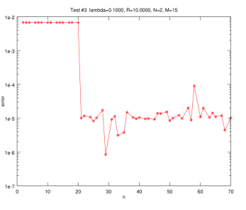
In all the experiments presented in Figures 1 and 2 below, we have fixed an a-priori randomly chosen exponential polynomial $H(s)$, and modified the sampling set $S$ according to the description of each experiment below. The sampling values $\{H(s_{i}),\;s_{i}\in S\}$ have been perturbed by the (random) amount $\varepsilon_{1}\sim 10^{-8}$. Subsequently, the least-squares approximation to $H(s)$ has been obtained by the standard sequential quadratic programming algorithm (implemented by the function sqp in GNU Octave environment). The initial values for the algorithm have been taken to be equal to the true values perturbed by the (random) amount $\varepsilon_{2}$, specified in each experiment below. We have plotted the recovery error for one of the frequencies (specifically, $|\Delta\phi_{2}|$).

In the first experiment we changed the distance $d$ between $s_{2},\dots,s_{n-1}$, while keeping the endpoints $s_{1},\;s_{n}$ (and thereby the value of $R$) fixed. The number of points was chosen to be exactly $n=M(2N,\lambda,R)+1$. According to Proposition 4.1, in this case we have $\omega(S)=d$. As can be seen in Figure 1, the error is roughly proportional to ${1\over\omega(S)}$.

In the second experiment, we have kept the endpoints of the set $S$ fixed ($0$ and $R$), while increasing the number $n$ of (equispaced) points in $S$. According to Figure 2, a significant improvement in accuracy appears when the number of samples passes $M(2N,\lambda,R)$ which is $15$ in this case.