Existence and nonuniqueness of segregated solutions to a class of cross-diffusion systems

Abstract

We study the the Dirichlet problem for the cross-diffusion system

$$\partial_{t}u_{i}=\operatorname{div}\left(a_{i}u_{i}\nabla(u_{1}+u_{2})\right)+f_{i}(u_{1},u_{2}),\quad i=1,2,\quad a_{i}=const>0,$$

in the cylinder $Q=\Omega\times(0,T]$. The functions $f_{i}$ are assumed to satisfy the conditions $f_{1}(0,r)=0$, $f_{2}(s,0)=0$, $f_{1}(0,r)$, $f_{2}(s,0)$ are locally Lipschitz-continuous. It is proved that for suitable initial data $u_{0}$, $v_{0}$ the system admits segregated solutions $(u_{1},u_{2})$ such that $u_{i}\in L^{\infty}(Q)$, $u_{1}+u_{2}\in C^{0}(\overline{Q})$, $u_{1}+u_{2}>0$ and $u_{1}\cdot u_{2}=0$ everywhere in $Q$. We show that the segregated solution is not unique and derive the equation of motion of the surface $\Gamma$ which separates the parts of $Q$ where $u_{1}>0$, or $u_{2}>0$. The equation of motion of $\Gamma$ is a modification of the Darcy law in filtration theory. Results of numerical simulation are presented.

• Keywords: Nonlinear parabolic equation, cross-diffusion system, segregated solutions, Lagrangian coordinates.

• AMS: 35K55, 35K57, 35K65, 35R35

1 Introduction

In the context of Population Dynamics, Gurney and Nisbet [15] derived from microscopic considerations the density-dependent population flux

$$J(u)=c\nabla u+au\nabla u,$$

with positive constants $a$ and $c$. In this expression the term $c\nabla u$ reflects a random dispersal of the population, while the population pressure $au\nabla u$ prevents overcrowding. The corresponding evolution equation has the form

$$\partial_{t}u-\operatorname{div}J(u)=u\left(\alpha-\frac{u}{\beta}\right),$$ (1)

where the right-hand side is the logistic growth term, $\alpha>0$ is the intrinsic growth rate and $\beta>0$ is the carrying capacity.

Various generalizations of this model were proposed, from different points of view, by Shigesada et al. [20], Busenberg and Travis [5], or [16, 11], among others, and have given rise to the so-called cross-diffusion models. The authors of [5] assume that the individual population flow $J_{i}$ is proportional to the gradient of a potential function $\Psi$ which depends only on the total population density $U=u_{1}+u_{2}$:

$$J_{i}(u_{1},u_{2})=a\frac{u_{i}}{U}\nabla\Psi(U).$$

In this model the collective flow is still given in the form (1): $J(U)=a\nabla\Psi(U)$ with $c=0$. Assuming the power law $\Psi(s)=s^{2}/2$, we arrive at the individual population flows given by

$$J_{i}(u_{1},u_{2})=au_{i}\nabla U.$$

This model was introduced by Gurtin and Pipkin [16] and mathematically analyzed by Bertsch et al. [2, 4]. As remarked in [16], when considering a set of species with different characteristics, such as size, behavior with respect to overcrowding, etc., it is natural to assume that instead of the total population density $u_{1}+u_{2}$ the individual flows $J_{i}$ depend on a general linear combination of both population densities, possibly different for each population. This assumption leads to the following expressions for the flows:

$$J_{i}(u_{1},u_{2})=u_{i}\nabla(a_{i1}u_{1}+a_{i2}u_{2}).$$ (2)

A more general evolution problem which included the flows of this type has been analyzed in [13]. A finite element fully discretized scheme was used to prove the existence of solutions under rather general assumptions on the data.

The present article addrresses the singular case $a_{ij}=a_{i}$ for $i,j=1,2$. Due to the loss of ellipticity of the diffusion matrix, this case is more complicated for the study. One of the possible approaches consists in considering the contact-inhibition problem, see [6], assuming that the components of the solution are initially segregated:

$$\operatorname{supp}u_{1}(x,0)\cup\operatorname{supp}u_{2}(x,0)=\Omega,\quad\operatorname{supp}u_{1}(x,0)\cap\operatorname{supp}u_{2}(x,0)=\Gamma_{0},$$ (3)

where $\Omega\subset\mathbb{R}^{n}$ is the problem domain and $\Gamma_{0}\in\Omega$ is a given hypersurface. In the one-dimensional case $\Omega=(-L,L)$ and $\Gamma_{0}=x_{c}\in(-L,L)$. A segregated solution $\mathbf{u}=(u_{1},u_{2})$ of the cross-diffusion system

$$\partial_{t}\mathbf{u}=\operatorname{div}\left(\mathbf{u}\nabla(A\cdot\mathbf{u}^{\perp})\right)+\mathbf{f}(\mathbf{u}),\quad\mathbf{f}=(f_{1},f_{2}),$$ (4)

with a $2\times 2$ matrix $A$, is a solution which possesses the following property: $u_{1}\cdot u_{2}=0$ and $u_{1}+u_{2}>0$ everywhere in the problem domain (we tacitly assume here that the solution is so regular that these conditions make sense). The problem of existence of segregated solutions of the cross-diffusion system (4) in the singular case $a_{ij}=1$ for $i,j=1,2$ was studied by Bertsch et.al. in [4]. It is proved that for suitable initial data the Cauchy problem for system (4) has a segregated solution. In [3] (see also [2]), the existence of segregated solutions was proved in the case $n=1$ for the system

$$u_{it}=a_{i}\left(u_{i}\phi_{x}(u_{1}+u_{2})\right)+f_{i}(u,v),\quad i=1,2,\quad a_{i}=const>0,$$ (5)

in the rectangular domain $(-L,L)\times(0,T]$ under the zero-flux boundary conditions for $u_{1}+u_{2}$ on the lateral boundaries. The proofs in [3, 4] rely on the observation that the introduction of the new thought function $w:=u_{1}+u_{2}$ transforms systems (4), (5) into systems composed of a parabolic equation for $w$ and a transport equation for the function $r:=u_{2}/w$ with the velocity field defined by $\nabla w$. Apart from the possibility to show the existence of segregated solutions, this method allowed the authors of [3] to derive the equation of motion of the curve $x=\zeta(t)$ separating the parts of the problem domain where either $u_{1}>0$, or $u_{2}>0$. The question of uniqueness of the segregated solutions for systems (4), (5) was left open.

2 Formulation of the problem and main results

Let $\Omega\subset\mathbb{R}^{n}$ be a bounded domain. We consider the problem of finding nonnegative functions $(u,v)$ satisfying the conditions

$$\begin{cases}&u_{t}=\operatorname{div}\left(a_{+}u\nabla(u+v)\right)+f_{+}(u,v)\quad\text{in $D=\Omega\times(0,T]$},\\ &v_{t}=\operatorname{div}\left(a_{-}v\nabla(u+v)\right)+f_{-}(u,v)\quad\text{in $D$},\quad a_{\pm}=const>0,\\ &\text{$u+v=h$ on $\partial\Omega\times(0,T]$},\\ &\text{$u(x,0)=u_{0}(x)$, $v(x,0)=v_{0}(x)$ in $\Omega$}.\end{cases}$$ (6)

It is assumed that the initial data are smooth and segregated:

$$\begin{cases}&\text{$u_{0}\geq 0$ and $v_{0}\geq 0$, $u_{0}\cdot v_{0}=0$ in $\overline{\Omega}$},\\ &\text{${C}^{-1}\leq u_{0}+v_{0}\leq C$ in $\Omega$, $\;C=const>1$},\\ &\text{$u_{0}+v_{0}\in C^{2+\alpha}(\overline{\Omega})$}.\end{cases}$$ (7)

Moreover, we assume that the supports of $u_{0}$ and $v_{0}$ are separated by a smooth simple-connected hypersurface $\Gamma_{0}$,

$$\Gamma_{0}=\partial\overline{\{x\in\Omega:\,v_{0}(x)>0\}},\qquad\Gamma_{0}\cap\partial\Omega=\emptyset,$$

which means that the domain $\Omega$ is split into two parts: the annular domain $\Omega_{+}$, bounded by $\partial\Omega$ and $\Gamma_{0}$ (where $v_{0}=0$, $u_{0}>0$), and its complement $\Omega_{-}$ (where $u_{0}=0$, $v_{0}>0$). The functions $f_{\pm}(q,r)$ are assumed to satisfy the conditions

$$\begin{cases}&f_{+}(0,r)=0,\quad\text{$f_{+}(q,0)$ is locally Lipschitz-continuous for $q\geq 0$},\\ &f_{-}(q,0)=0,\quad\text{$f_{-}(0,r)$ is locally Lipschitz-continuous for $r\geq 0$},\end{cases}$$ (8)

an example of admissible $f_{\pm}$ is furnished by the functions

$$f_{+}(q,r)=q(\alpha_{+}-\beta_{+}q-\gamma_{+}r),\quad f_{-}(q,r)=r(\alpha_{-}-\beta_{-}q-\gamma_{-}r),$$

$\alpha_{\pm},\beta_{\pm},\gamma_{\pm}=const>0$. Our aim is to construct a segregated solution of problem (6). To this end we consider the initial and boundary value problem for function $w=u+v$. If problem (6) admits a segregated solution such that $u+v>0$ and $u\cdot v=0$ everywhere in $\overline{D}$, it is necessary that $w$ satisfies the conditions

$$\begin{cases}&w_{t}=\operatorname{div}\left(a\,w\nabla w\right)+f(w)\quad\text{in $D=\Omega\times(0,T]$},\\ &\text{$w=h$ on $\partial\Omega\times(0,T]$},\\ &\text{$w(x,0)=w_{0}:=u_{0}+v_{0}$ in $\Omega$}\end{cases}$$ (9)

with the coefficient $a$ and the right-hand side $f$ defined by

$$a=\begin{cases}a_{+}&\text{if $u>0$},\\ a_{-}&\text{if $v>0$},\end{cases}\qquad f(w)=\begin{cases}f_{+}(w,0)&\text{$u>0$},\\ f_{-}(0,w)&\text{if $v>0$}.\end{cases}$$ (10)

Problem (9) is regarded as the initial and boundary value problem for a parabolic equation with discontinuous data. If there is a continuous in $D$ solution $w$, and if there exists a continuous bijective transformation $\Gamma_{0}\mapsto\Gamma_{t}$ of the initially given surface $\Gamma_{0}$, we may try to define a solution of the original problem (6) by the equalities

$$w(x,t)=\begin{cases}v(x,t)&\text{in the domain $\Omega^{-}(t)$ bounded by $\Gamma_{t}$, $t\in[0,T]$},\\ u(x,t)&\text{in the complement $\Omega^{+}(t)$ of $\Omega^{-}(t)$ in $\Omega$}.\end{cases}$$

Definition 2.1.

A pair $(w,\Gamma)$ is called weak solution of problem (9) if

1. $\Gamma$ is a $C^{1}$ hypersurface, the mapping $\Gamma_{0}\mapsto\Gamma_{t}=\Gamma\cap\{t=const\}$ is a bijection for $t\in[0,T]$,

2. $\forall\;t\in[0,T]$ the surface $\Gamma_{t}$ is the common boundary of the domains $\Omega^{\pm}(t)$,

   $$\Omega=\Omega^{+}(t)\cup\Gamma_{t}\cup\Omega^{-}(t),$$

   where $\Omega^{+}(t)$ is an annular domain bounded by $\partial\Omega$ and $\Gamma_{t}$, $\Omega^{-}(t)$ is the complement of $\Omega^{+}(t)$ in $\Omega$,

3. $w\in C^{0}(\overline{D})\cap L^{2}(0,T;H^{1}(\Omega^{\pm}(t)))$,

4. for every $\phi(x,t)\in C^{1}(\overline{D})$, such that $\phi(x,T)=0$, $\phi=0$ on $\partial\Omega\times[0,T]$,

   $$\int_{D}\left(w\phi_{t}-aw\nabla w\cdot\nabla\phi+f(w)\,\phi\right)\,dxdt+\int_{\Omega}w_{0}\phi(x,0)dx=0.$$ (11)

To construct a solution of problem (9) we proceed in two steps. The first step consists in the direct construction of the surface $\Gamma$ and the corresponding solution $w$ in a vicinity of $\Gamma$. This is done by means of a special coordinate transformation similar to introduction of a system of Lagrangian coordinates frequently used in continuum mechanics. Once the local solution is constructed, we continue it to the rest of the problem domain and then check that this continuation is the thought solution of problem (9).

Theorem 2.2 (Local in time existence-1).

Let conditions (7), (8) be fulfilled. Assume that the data of problem (9) satisfy the following conditions:

1. $\partial\Omega,\,\Gamma_{0}\in C^{2+\alpha}$, $w_{0}\in C^{2+\alpha}(\Omega)$ with some $\alpha\in(0,1)$,

2. $\Gamma_{0}$ is a level surface of $w_{0}$,

3. $h(x,t)>0$ on $\partial\Omega\times[0,T]$, $h(x,t)$ and $w_{0}(x)$ satisfy the first-order compatibility conditions on $\partial\Omega\times\{t=0\}$.

Then for every $\Phi(t)\in C^{1}[0,T]$

1. there exists $T^{\ast}\leq T$ such that in the cylinder $\Omega\times(0,T^{\ast}]$ problem (9) has a solution $w(x,t)$ in the sense of Definition 2.1, which satisfies the condition $w=\Phi(t)$ on $\Gamma_{t}$,

2. the solution $w$ represents the segregated solution $(u,v)$ of system (6): $w=u+v$, $u\equiv 0$ in $\Omega^{-}(t)\times[0,T^{\ast}]$, $v\equiv 0$ in $\Omega^{+}(t)\times[0,T^{\ast}]$.

The method of construction allows us to present the surface $\Gamma$ explicitly and to derive the equation of motion of $\Gamma_{t}$, which is similar to the Darcy law in filtration theory.

Theorem 2.3 (The interface equation).

Under the conditions of Theorem 2.2 there exists an annular domain $\omega^{+}(0)$, bounded by $\Gamma_{0}$ and a smooth hypersurface $\partial\omega^{+}(0)$, $\partial\omega^{+}(0)\cap\partial\Omega=\emptyset$, $\partial\omega^{+}(0)\cap\Gamma_{0}=\emptyset$, and a function $U(y,t)$ such that

$$U\in W^{4}_{q}(\omega^{+}(0)\times[0,T^{\ast}]),\quad U_{t}\in W^{2}_{q}(\omega^{+}(0)\times[0,T^{\ast}]),\quad\text{$U(y,0)=0$ in $\overline{\omega}^{+}(0)$}$$

with some $q>n+2$, and $\Gamma$ is parametrized by the equalities

$$\Gamma=\{(x,t):\,x=y+\nabla U(y,t),\,y\in\Gamma_{0}\},\quad t\in[0,T^{\ast}].$$

Moreover, the velocity of advancement of the surface $\Gamma_{t}$ in the normal direction $\mathbf{n}_{x}$ is defined by the equation

$$\mathbf{v}\cdot\mathbf{n}_{x}=(-a_{+}\nabla u+\nabla p)\cdot\mathbf{n}_{x}|_{\Gamma_{t}}\quad(\text{the modified Darcy law}),$$ (12)

where $p$ is a solution of the elliptic equation

$$\begin{cases}&\text{$\operatorname{div}\left(u\nabla p\right)=f_{+}(u)$ in $\omega^{+}(t)=\{x\in\Omega:\,x=y+\nabla U,\,y\in\omega^{+}(0)\}$},\\ &\text{$p=0$ on $\Gamma_{t}$ and $\partial\omega^{+}(t)$}.\end{cases}$$

Corollary 1.

The components $u$ and $v$ of the solution $w=u+v$ to problem (9) constructed in Theorem 2.2 can be characterized in the following way:

1. $u,\,v\in L^{\infty}(D)$, $u\geq 0,\,v\geq 0$ in $D$,

2. $u+v\in C^{0}(\overline{D})$, $u+v\in L^{2}(0,T;H^{1}(\Omega))$,

3. for every test-function $\phi\in C^{1}(\overline{D})$, $\phi(x,T)=0$, $\phi=0$ on $\partial\Omega\times[0,T]$,

   $$\int_{D}\left(u\phi_{t}-a_{+}u\nabla(u+v)\cdot\nabla\phi+f_{+}(u)\,\phi\right)\,dxdt+\int_{\Omega}u_{0}\phi(x,0)dx=0,$$ (13)

   $$\int_{D}\left(v\phi_{t}-a_{-}v\nabla(u+v)\cdot\nabla\phi+f_{-}(v)\,\phi\right)\,dxdt+\int_{\Omega}v_{0}\phi(x,0)dx=0$$ (14)

(cf. with Definition 3.1 in [4]). The proof of this assertion is given in the end of Section 5.

Theorem 2.4 (Nonuniqueness).

Under the conditions of Theorem 2.2 the segregated solution of probem (6) is not unique.

The assertion of Theorem 2.4 is an immediate byproduct of Theorem 2.2. Indeed: given $u_{0}$, $v_{0}$ and a level surface $\Gamma_{0}$ of the function $w_{0}=u_{0}+v_{0}$, for every smooth $\Phi(t)$ such that $\Phi(0)=w_{0}|_{\Gamma_{0}}$ we obtain a new solution of problem (6) corresponding to the same initial data and satisfying the condition $w=\Phi(t)$ on $\Gamma_{t}$.

The assumptions that $w=\Phi(t)$ on $\Gamma_{t}$ and that $\Gamma_{0}$ is a level surface of $w_{0}=u_{0}+v_{0}$ are not essential for the proof of Theorem 2.2 and were included in order to make evident nonuniqueness of segregated solutions of problem (9).

Theorem 2.5 (Local in time existence-2).

Let conditions (7), (8) be fulfilled. Assume that the data of problem (9) satisfy the following conditions:

1. $\partial\Omega,\,\Gamma_{0}\in C^{2+\alpha}$, $w_{0}\in C^{2+\alpha}(\Omega)$ with some $\alpha\in(0,1)$,

2. $h(x,t)>0$, $h$ and $w_{0}$ satisfy the first-order compatibility conditions on $\partial\Omega\times\{t=0\}$.

Then there exists $T^{\ast}\leq T$ such that in the cylinder $\Omega\times(0,T^{\ast}]$ problem (9) has a solution in the sense of Definition 2.1. The solution $w$ of problem (9) represents the segregated solution $(u,v)$ of system (6): $w=u+v$, $u\equiv 0$ in $\Omega^{-}(t)\times[0,T^{\ast}]$, $v\equiv 0$ in $\Omega^{+}(t)\times[0,T^{\ast}]$. Moreover, for the interface of the constructed solution Theorem 2.3 holds.

Remark 1.

It is worth noting here that the choice of the Dirichlet boundary condition in (6) is mostly the question of convenience. The assertions of Theorems 2.2-2.5 remain true if the boundary condition in (6) is substituted by any other condition which allows one to guarantee that the auxiliary problem (54) below has a regular solution. In particular, we may pose the no-flux conditions for $u+v$ on $\partial\Omega\times[0,T]$.

The proofs of the main results are based on a special nonlocal coordinate transformation which is similar to introduction of the system of Lagrangian coordinates in continuum mechanics. The change of independent variables allows us to reduce the construction of the moving boundary $\Gamma$ (the interface) to a problem posed in a time-independent domain. We follow the ideas of [7, 8], see also [22, 21, 23] where the method of Lagrangian coordinates was applied to the study of free boundary problems for nonlinear parabolic equations with degeneracy on the interface.

Organization of the paper. In Section 3 we introduce a local system of Lagrangian coordinates. In the new coordinate system the problem of finding the surface $\Gamma$ and the solution of problem (9) in a vicinity of $\Gamma$ transforms into an equivalent problem posed in a time-independent cylinder. In the new formulation the interface $\Gamma$ becomes a vertical surface. The new problem is a system of nonlinear evolution equations which is solved in Section 4. In Section 5 we give the proofs of the main theorems. Finally in Section 6 we give an account of the available results on the problems of the type (5) without the contact inhibition assumption and present some results on the numerical simulation of solution to system (6) which correspond to the segregated initial data.

3 Local system of lagrangian coordinates

Let us consider the following auxiliary problem: to find a strictly positive function $w(x,t)$, a family of annular domains $\{\omega^{\pm}(t)\}_{t>0}$, and the surface

$$\Gamma=\bigcup_{t>0}\Gamma_{t},\qquad\Gamma_{t}=\overline{\omega}^{+}(t)\cap\overline{\omega}^{-}(t),$$

satisfying the conditions

$$\begin{cases}&\partial_{t}w-\operatorname{div}(a\,w\,\nabla w)=f(w)\quad\text{in $\mathcal{C}^{\pm}=\bigcup_{t>0}\omega^{\pm}(t)$},\\ &[w]|_{\Gamma_{t}}=0,\\ &\text{$w(x,0)=w_{0}(x)$ in $\omega^{\pm}(0)$},\\ &\displaystyle\int_{\omega^{\pm}(t)}w(x,t)\,dx=\int_{\omega^{\pm}(0)}w_{0}(x)\,dx\quad\forall\,t\in(0,T]\end{cases}$$ (15)

Here and throughout the rest of the paper the symbol $[\phi]_{\gamma}$ means the jump of the function $\phi$ across the surface $\gamma$. The surface $\Gamma_{0}$ is the common boundary of the annular domains $\omega^{\pm}(0)$. The exterior boundary of $\omega^{+}(0)$ is denoted by $\partial\omega^{+}(0)$, $\partial\omega^{-}(0)$ stands for the interior boundary of $\omega^{-}(0)$. Notice that problem (15) includes three unknown boundaries: the interface $\Gamma$ and $\bigcup\limits_{t>0}\partial\omega^{\pm}(t)$.

We will use the notations $\omega(t)=\omega^{+}(t)\cup\Gamma_{t}\cup\omega^{-}(t)$ and $\mathcal{C}=\mathcal{C}^{+}\cup\mathcal{C}^{-}$.

Definition 3.1.

A pair $(w,\,\mathcal{C})$ is called weak solution of problem (15) if

• $w\in C^{0}(\overline{\mathcal{C}})\cap L^{2}(0,T;H^{1}(\omega(t)))$,

• $\forall\,\phi\in C^{1}(\overline{\mathcal{C}})$, such that $\phi(x,T)=0$ and $\phi=0$ on $\partial\omega^{\pm}(t)\times[0,T]$,

  $$\begin{split}\int_{\mathcal{C}}(w\,\phi_{t}-a\,w\,\nabla w\cdot\nabla\phi+\phi\,f)\,dxdt&+\int_{\omega(0)}\phi(x,0)w_{0}\,dx=0.\end{split}$$ (16)

3.1 A coordinate transformation in a moving annular domain

Let us consider the problem of defining the family of transformations $X(y,t):\,S(0)\mapsto S(t)$ of an open annular set $S(0)\subset\mathbb{R}^{n}$ and a function $w(x,t)$ according to the following conditions:

• for every $t>0$

  $$\text{$X(y,t):\,\overline{S(0)}\mapsto\overline{S(t)}\subset\mathbb{R}^{n}$ is a diffeomorphism},$$ (17)

  that is $S(t)=X(S(0),t)$, $S(0)=X^{-1}(S(t),t)$, $\partial S(t)=X(\partial S(0),t)$,

• the deformation of $S(t)$ is governed by the differential equation

  $$\begin{cases}&\operatorname{div}_{x}\,(w\,(X_{t}(y,t)-\mathbf{v}(X(y,t),t)))=0\quad\text{for a.e.}\,y\in S(0),\,t>0,\\ &X(y,0)=y\in S(0),\end{cases}$$ (18)

  with a given vector-field $\mathbf{v}(x,t):\,S(t)\times[0,T]\mapsto\mathbb{R}^{n}$ in the sense that for every $\phi\in C^{1}(0,T;C_{0}^{1}(S(t)))$

  $$\int_{S(t)}w\nabla\phi\cdot(X_{t}(y,t)-\mathbf{v}(X(y,t),t))\,dx=0,\quad t>0,$$

• for every subset $\sigma(0)\subset S(0)$ its image $\sigma(t)$ at the instant $t\geq 0$ is connected with the function $w(x,t)$ by the formula

  $$\int_{\sigma(0)}w(x,0)\,dx=\int_{\sigma(t)}w(x,t)\,dx.$$ (19)

Let $J$ be the Jacobian matrix of the mapping $y\to X(y,t)$, $|J|\not=0$ because of (17). By agreement we always denote

$$\widetilde{g}(y,t)=\left.g(x,t)\right|_{x=X(y,t)},$$

so that $\widetilde{w}(y,t)\equiv w[X(y,t),t]\equiv w(x,t)$. Take an arbitrary set $\sigma(0)\subseteq S(0)$ and denote $\sigma(t)=X(\sigma(0),t)$. For a.e. $t>0$

$$\begin{split}0&=\dfrac{d}{dt}\left(\int_{\sigma(t)}w(x,t)\,dx\right)\\ &=\dfrac{d}{dt}\left(\int_{\sigma(0)}\widetilde{w}(y,t)\,|J|\,dy\right)=\int_{\sigma(0)}\dfrac{d}{dt}\left(\widetilde{w}(y,t)\,|J|\right)\,dy,\end{split}$$ (20)

provided that $|J|$ is continuous as a function of $y$. Since $\sigma(0)$ is arbitrary and $|J(y,0)|=1$, it is necessary that

$$\widetilde{w}(y,t)\,|J(y,t)|=w(y,0)\quad\text{for a.e. $y\in S(0)$, $t>0$}.$$ (21)

Lemma 3.2.

Assume that

1. $X$ satisfy (17), $|J(y,t)|\in C^{0}(S(0))$ and $|J(y,t)|\not=0$ in $S(0)$ for a.e. $t\in(0,T)$,

2. equations (18) and (21) are fulfilled a.e. in the cylinder $S(0)\times(0,T)$,

3. $\widetilde{w}\cdot(X_{t}-\mathbf{v}(X,t))\in(L^{\infty}(S(0)))^{n}$ for a.e. $t\in(0,T)$,

4. $\partial S(t)\in Lip$ for a.e. $t\in(0,T).$

Then the function $w(x,t)|_{x=X(y,t)}=\widetilde{w}(y,t)$ defined by (21) satisfies the conditions

$$\begin{cases}&w_{t}-\operatorname{div}\,(w\,\mathbf{v}(x,t))=0\quad\text{in $\mathcal{D}\equiv\bigcup_{t\in(0,T)}X(S(0),t)$},\\ &\text{$w(x,0)=w_{0}(x)$ in $S(0)$}\end{cases}$$ (22)

in the following sense: $\forall\,\phi\in C^{1}(0,T;C_{0}^{1}(\mathbb{R}^{n}))$, $\phi(x,T)=0$, $\phi=0$ on $\partial S(t)\times[0,T]$,

$$\begin{split}\int_{S(0)}w_{0}(x)\,\phi(x,0)\,dx&+\int_{\mathcal{D}}w\,\left(\phi_{t}+\nabla_{x}\phi\cdot\mathbf{v}(x,t)\right)\,dxdt=0.\end{split}$$ (23)

Proof.

By [10, Th.2.2] for a.e. $t>0$ the field $F:=w\,(X_{t}-\mathbf{v}(X,t))$ has the normal traces on every Lipschitz-continuous surface in $\overline{S(t)}$ and the Green-Gauss formulas hold: for every $\phi\in C^{1}(0,T;C_{0}^{1}(S(t)))$

$$0=\int_{S(t)}\phi\,\operatorname{div}\,F\,dx=-\int_{S(t)}\nabla\phi\cdot F\,dx.$$

Let us denote $D_{T}=S(0)\times(0,T]$. Notice that for every test-function $\phi\in C^{\infty}(0,T;C_{0}^{1}(S(t)))$, vanishing as $t=T$,

$$\left.\dfrac{d}{dt}\phi(x,t)\right|_{x=X(y,t)}=\widetilde{\phi}_{t}(y,t)+\widetilde{\nabla_{x}\phi(x,t)}\cdot X_{t}.$$

Then

$$\begin{split}-\int_{S(0)}w_{0}(y)\,\phi(y,0)\,dy&=\int_{0}^{T}\dfrac{d}{dt}\left(\int_{S(t)}w(x,t)\,\phi(x,t)\,dx\right)\,dt\\ &=\int_{0}^{T}\dfrac{d}{dt}\left(\int_{S(0)}\widetilde{w}(y,t)\,\widetilde{\phi}(y,t)\,|J|\,dy\right)\,dt\\ &=\int_{D_{T}}\dfrac{d}{dt}\left(\widetilde{w}(y,t)\,\widetilde{\phi}(y,t)\,|J|\right)\,dydt\\ &=\int_{D_{T}}\left[\dfrac{d}{dt}\left(\widetilde{w}(y,t)|J|\right)\widetilde{\phi}+\widetilde{w}\,(\widetilde{\phi_{t}}+\widetilde{\nabla_{x}\phi}\cdot X_{t})\,|J|\right]\,dydt.\end{split}$$

Using (21) we obtain

$$\begin{split}-\int_{S(0)}w_{0}(y)\,\phi(y,0)\,dy&=\int_{D_{T}}\widetilde{w}\,(\phi_{t}+\widetilde{\nabla_{x}\phi}\cdot X_{t})\,|J|\,dydt\\ &=\int_{D_{T}}\widetilde{w}\,\left(\widetilde{\phi_{t}}+\widetilde{\nabla_{x}\phi}\cdot\mathbf{v}(X,t)\right)\,|J|\,dydt\\ &=\int_{0}^{T}\int_{S(t)}w\,\left(\phi_{t}+\nabla_{x}\phi\cdot\mathbf{v}(x,t)\right)\,dxdt.\end{split}$$ (24)

∎

Theorem 3.3.

Assume that the domain $\omega(0)$ is split into two annular domains $\omega^{\pm}(0)$ by the Lipschitz-continuous surface $\Gamma_{0}$ such that $\Gamma_{0}\cap\partial\omega^{\pm}(0)=\emptyset$. If the conditions of Lemma 3.2 are fulfilled in each of the domains $\omega^{\pm}(0)$ and if

1. $\lim\limits_{\omega^{+}(0)\ni y\to y_{0}\in\Gamma_{0}}|J(y,t)|=\lim\limits_{\omega^{-}(0)\ni y\to y_{0}\in\Gamma_{0}}|J(y,t)|\quad\forall\,y_{0}\in\Gamma_{0},\;t\in[0,T]$,

2. $\mathbf{v}\in C^{0}(\overline{\omega^{+}(t)\cup\omega^{-}(t)})\times[0,T];\,\mathbb{R}^{n})$,

then $w(x,t)$ defined by (21) satisfies conditions (22) in the sense of (23).

Proof.

By Lemma 3.2 problem (22) has solutions $w^{\pm}$ in each of the domains $\mathcal{C}^{\pm}$. By virtue of condition (ii) the images of the surface $\Gamma_{0}$ under the mappings $X^{+}$ and $X^{-}$ coincide, which means that $\Gamma_{t}=\overline{\mathcal{C}}^{+}\cap\overline{\mathcal{C}}^{+}$. The function $w(x,t)=\widetilde{w}(y,t)$ defined by (21) in each of the domains $\mathcal{C}^{\pm}$ is continuous across the surface $\Gamma_{t}$ because of assumption (i). Finally, to get (22) we gather relations (24), corresponding to the domains $\omega^{\pm}(0)$. ∎

Theorem 3.3 will be used in the proof of Theorem 2.5. In the proof of Theorem 2.2 we rely on the following version of Theorem 3.3.

Theorem 3.4.

The assertion of Theorem 3.3 remains true if condition (ii) is substituted by the conditions

• $\quad w(x,t)=\Phi(t)$ on $\Gamma_{t}$, $\qquad[\mathbf{v}\cdot\mathbf{n}_{x}]_{\Gamma_{t}}=0$,

where $\mathbf{n}_{x}$ denotes the unit normal vector directed inward $\omega^{-}(t)$, and $\Phi(t)$ is a given strictly positive function.

Proof.

The assertion follows from Lemma 3.2: although the tangential component of the velocity is no longer continuous across $\Gamma_{t}$, the assumption $w=\Phi(t)$ on $\Gamma_{t}$ provides continuity of the flux $w\,(\mathbf{v}\cdot\mathbf{n}_{x})$ across $\Gamma_{t}$. ∎

3.2 Potential flows

Let us now search for the fields $X(y,t)$ and $\mathbf{v}(X,t)$ in the potential form:

$$\begin{split}&\text{$X(y,t)=y+\nabla_{y}U$ in $\omega^{\pm}(0)\times[0,T]$},\\ &\text{$\mathbf{v}(x,t)=-a_{\pm}\,\nabla_{x}w+\nabla_{x}p$ in $\omega^{\pm}(0)\times[0,T]$},\\ &\text{$U=0$ on the parabolic boundaries of $\omega^{\pm}(0)\times[0,T]$},\end{split}$$ (25)

where $U(y,t)$ and $w(x,t)=\widetilde{w}(y,t)$ are scalar functions related by (21) and $p(x,t)$ is the new unknown. The parabolic boundary of a cylinder means “the lateral boundaries and the bottom”. For every $\phi\in C^{1}(0,T;C_{0}^{1}(\omega(t)))$, $\phi(x,T)=0$, $\phi=0$ on $\partial\mathcal{C}$,

$$\int_{\omega(0)}w_{0}\,\phi(x,0)\,dx+\int_{\mathcal{C}}\left(w\,\phi_{t}-a\,w\,\nabla_{x}\phi\cdot\nabla_{x}w\right)\,dx+\int_{\mathcal{C}}w\,\nabla_{x}\phi\cdot\nabla_{x}p\,dx=0.$$ (26)

Let us take for $p$ a solution of the elliptic equation endowed with the Dirichlet boundary conditions on $\partial\omega^{\pm}(t)$ and satisfying the additional condition on $\Gamma_{t}$, which provides continuity of the flux $\Phi(t)\,\left(\mathbf{v}\cdot\mathbf{n}_{x}\right)$ across the moving boundary:

$$\begin{cases}&-\operatorname{div}_{x}\left(w\,\nabla_{x}p\right)=f(w)\quad\text{in $\omega^{\pm}(t)$},\\ &\text{$p=0$ on $\partial\omega^{\pm}(t)$},\\ &[\nabla_{x}p\cdot\mathbf{n}_{x}]_{\Gamma_{t}}=[a\,\nabla_{x}w\cdot\mathbf{n}_{x}]_{\Gamma_{t}}.\end{cases}$$ (27)

Then for every smooth $\phi$, such that $\phi(x,T)=0$, $\phi=0$ on $\partial\mathcal{C}$,

$$\int_{\omega(0)}w_{0}\,\phi(x,0)\,dx+\int_{\mathcal{C}}\left(w\,\phi_{t}-a\,w\,\nabla_{x}\phi\cdot\nabla_{x}w+f\,\phi\right)\,dx=0.$$ (28)

Let us formulate the conditions for $U$ and $P=\widetilde{p}$ in the time-independent annular cylinders

$$Q^{\pm}_{T}=\omega^{\pm}(0)\times[0,T].$$

Denote by $J$ the Jacobian matrix of the mapping $x=y+\nabla U$. Applying Lemma 3.2 we have that for every test-function $\phi(x,t)=\phi(X(y,t),t)=\widetilde{\phi}(y,t)$, $\phi\in C^{0}(0,T;C^{1}_{0}(\omega(t)))$, $\phi=0$ on $\partial\omega(t)$,

$$\begin{split}0&=\int_{\omega^{\pm}(t)}\phi\,\operatorname{div}_{x}\,(w\,(\nabla_{y}U_{t}+a_{-}\widetilde{\nabla_{x}w}-\widetilde{\nabla_{x}p})\,dx\\ &=-\int_{\omega^{\pm}(0)}\left[w_{0}((J^{-1})^{2}\cdot\nabla_{y}\widetilde{\phi})\cdot\left(J\cdot\nabla_{y}U_{t}+a\,\nabla_{y}\left(w_{0}|J|^{-1}\right)-\nabla_{y}\widetilde{p}\right)\right]\,dy.\end{split}$$

In particular, if $w_{0},\,J_{ij}\in C^{\alpha}(\omega^{\pm}(0))$, and if $|J|$ is separated away from zero, we may take for $\phi$ a solution of the problem

$$\begin{cases}&\text{$\operatorname{div}_{y}\left(w_{0}(J^{-1})^{2}\cdot\nabla_{y}\widetilde{\phi}\right)=\Delta_{y}\widetilde{\psi}$ in $\omega^{\pm}(0)$},\\ &\text{$\phi=0$ on $\partial\omega^{\pm}(0)$}\end{cases}$$

with an arbitrary $\psi\in C^{0}(0,T;C^{1}_{0}(\omega(0)))$, whence

$$\int_{\omega^{\pm}(0)}\psi\,\operatorname{div}_{y}\left(J\cdot\nabla_{y}U_{t}+a_{+}\nabla_{y}\left(w_{0}|J|^{-1}\right)-\nabla_{y}\widetilde{p}\right)\,dy=0$$

and

$$\begin{cases}&\qquad\mathcal{L}(U,\widetilde{p})\equiv\operatorname{div}_{y}\left(J\cdot\nabla_{y}U_{t}+a\nabla_{y}\left(w_{0}|J|^{-1}\right)-\nabla_{y}\widetilde{p}\right)=0\quad\text{in $Q^{\pm}_{T}$},\\ &(a)\quad\text{$U=0$ on the parabolic boundaries of $Q_{T}^{\pm}$},\\ &(b)\quad\text{$\Phi(t)|J|_{\Gamma_{0}}=\Phi(0)$ for all $t\in[0,T]$}.\end{cases}$$ (29)

The boundary condition (29) (b) follows from (21) and the condition $w=\Phi(t)$ on $\Gamma_{t}$. (If we assume the conditions of Theorem 2.5, this condition is omitted). Proceeding in the same way we transform the problem for $\widetilde{p}(y,t)=p(x,t)$ into the problem posed in the time-independent domains $\omega^{\pm}(0)$:

$$\begin{cases}&\qquad\mathcal{M}(\widetilde{p},U)\equiv-\operatorname{div}_{y}\left(w_{0}(J^{-1})^{2}\nabla_{y}\widetilde{p}\right)+{f}(w_{0}|J^{-1}|)|J|=0\\ &\qquad\qquad\qquad\text{in $\omega^{\pm}(0)$ for a.e. $t\in(0,T]$},\\ &(a)\quad\text{$\widetilde{p}=0$ on $\partial\omega^{\pm}(0)$},\\ &(b)\quad[J^{-1}\cdot\nabla_{y}\widetilde{p}\cdot\widetilde{\mathbf{n}}_{x}]_{\Gamma_{0}}=[a\,J^{-1}\cdot\nabla_{y}(w_{0}|J^{-1}|)\cdot\widetilde{\mathbf{n}}_{x}]_{\Gamma_{0}}.\end{cases}$$ (30)

Condition (30) (b) provides continuity of the normal component of the velocity $\mathbf{v}$ across the moving boundary $\Gamma_{t}$.

Theorem 3.5.

Let us assume that problem (29)-(30) has a solution $(U,\widetilde{p})$ such that the conditions of Lemma 3.2 are fulfilled with

$$X=y+\nabla_{y}U\quad\text{ and}\quad\mathbf{v}=-a\,\nabla_{x}w+\nabla_{x}p.$$ (31)

Then the function $w(x,t)$ defined by the formulas

$$\begin{cases}&\mathcal{C}^{\pm}=\left\{(x,t):\,x=y+\nabla_{y}U(y,t),\,(y,t)\in Q^{\pm}_{T}\right\},\\ &w(x,t)={w_{0}(y)}{|J^{-1}|},\end{cases}$$ (32)

is a solution of problem (15) in the sense of Definition 3.1. The moving boundaries of $\mathcal{C}$ and the interface $\Gamma$ are parametrized by the equations

$$x|_{\Gamma_{t}}=y|_{\Gamma_{0}}+\nabla_{y}U(y,t)|_{\Gamma_{0}},\qquad x|_{\partial\omega^{\pm}(t)}=y|_{\partial\omega^{\pm}(0)}+\nabla_{y}U(y,t)|_{\partial\omega^{\pm}(0)}.$$

The proof is an immediate byproduct of Theorem 3.4.

3.3 Splitting the problems in the annular cylinders $Q_{T}^{\pm}$

The next step is to split the nonlinear system (29)-(30) into two similar systems in the annular cylinders $Q_{T}^{\pm}$ which can be solved sequentially. Let us consider first the following problem for defining $(U^{+},P^{+})$:

$$\begin{cases}&\text{$\mathcal{L}(U^{+},P^{+})=0$ in $Q_{T}^{+}$},\\ &\text{$\mathcal{M}(P^{+},U^{+})=0$ in $\omega^{+}(0)$},\\ &\text{$U^{+}=0$ on the parabolic boundary of $Q_{T}^{+}$},\\ (\ast)&\text{$|J|=\dfrac{\Phi(0)}{\Phi(t)}\equiv\Psi(t)$ on $\Gamma_{0}\times[0,T]$},\\ &\text{$P^{+}=0$ on $\partial\omega^{+}(0)$ and $\Gamma_{0}$ for all $t\in[0,T]$}.\end{cases}$$ (33)

Let us assume that problem (33) has a solution $(U^{+},P^{+})$ which satisfies the regularity assumptions of Lemma 3.2. The function $P^{+}$ automatically satisfies then the boundary condition (30) (a) on the lateral boundaries of $Q_{T}^{+}$. Given a pair $(U^{+},P^{+})$, we may formulate the problem for $(U^{-},P^{-})$ in $Q_{T}^{-}$, which should include the conditions of zero jumps of density and the normal velocity across the interface $\Gamma_{t}$. The problem in $Q_{T}^{-}$ is formulated as follows:

$$\begin{cases}&\text{$\mathcal{L}(U^{-},P^{-})=0$ in $Q_{T}^{-}$},\\ &\text{$\mathcal{M}(P^{-},U^{-})=0$ in $\omega^{-}(0)$},\\ &\text{$U^{-}=0$ on the parabolic boundary of $Q_{T}^{-}$},\\ (\ast\ast)&\text{$|J^{-}|=\Psi(t)$ on $\Gamma_{0}\times(0,T]$},\\ &\text{$P^{-}=0$ on $\partial\omega^{-}(0)$},\\ &\text{$[J^{-1}\cdot\nabla_{y}P\cdot\widetilde{\mathbf{n}^{+}_{x}}]_{\Gamma_{0}}=[a\,J^{-1}\cdot\nabla_{y}(w_{0}|J^{-1}|)\cdot\widetilde{\mathbf{n}^{+}_{x}}]_{\Gamma_{0}}$ for $t\in[0,T]$},\end{cases}$$ (34)

where the upper index “+” indicates that the corresponding magnitudes are already defined by the functions $(U^{+},P^{+})$. By $\widetilde{\mathbf{n}^{+}_{x}}$ we denote the exterior normal vector to the hypersurface $\Gamma_{t}$ parametrized by the formula $X=(y+\nabla U^{+})|_{y\in\Gamma_{0}}$. The vector $\widetilde{\mathbf{n}^{+}}_{x}$ is well-defined if $\Gamma_{0}\in C^{2+\alpha}$ - see Remark 4 below. Once problems (33), (34) are solved, the functions

$$U=\begin{cases}U^{+}&\text{in $Q^{+}_{T}$},\\ U^{-}&\text{in $Q^{-}_{T}$},\end{cases}\qquad\qquad\widetilde{p}=\begin{cases}P^{+}&\text{in $Q^{+}_{T}$},\\ P^{-}&\text{in $Q^{-}_{T}$}\end{cases}$$

define a solution of problem (29)-(30).

Due to Theorem 3.5, to solve problem (15) it suffices to construct functions $U^{\pm}$, $P^{\pm}$ that satisfy the assumptions of Theorem 3.4 (or Theorem 3.3).

Remark 2.

Let the conditions of Theorem 2.5 be fulfilled. In order to construct a solution of problem (9) we omit condition $(\ast)$ in (33) and substitute condition $(\ast\ast)$ in (34) by

$$|J^{-}|=|J^{+}| \Gamma_{0}\times[0,T] (i)$$ on       (condition of Theorem 3.3) (35)

Condition $(ii)$ of Theorem 3.3 has to be checked a posteriori.

4 Problem in the annular cylinder $Q_{T}^{+}$

Nonlinear problems similar to (33), (34) were already studied in [7, 8]. By this reason we confine ourselves to presenting the main ideas of the proofs and omit the technical details.

We begin with problem (33) posed in $Q_{T}^{+}$. To decouple the system of equations for $U^{+}$ and $P^{+}$ we solve first the nonlinear equation $\mathcal{L}(U^{+},P)=0$ considering $P$ as a given function from a suitable function space, and then solve the linear elliptic equation $\mathcal{M}(P^{+},U)=0$ with a given $U$. The solutions of these equations generate an operator $\chi:\,(U,P)\mapsto(U^{+},P^{+})$. We show that the operator $\chi$ has a fixed point, which is the sought solution of system (33).

4.1 The function spaces

Let $q>n+2$. We introduce the Banach spaces

$$\begin{split}&\displaystyle\mathcal{Z}^{+}=\left\{U:\;\begin{array}[c]{l}U\in W^{4}_{q}(Q_{T}^{+}),\;U_{t}\in W^{2}_{q}(Q_{T}^{+}),\\ \mbox{$U=0$ on the parabolic boundary of $Q_{T}^{+}$}\end{array}\right\},\\ &\mathcal{Y}^{+}=\left\{f:\;f\in W^{2}_{q}(Q_{T}^{+})\right\},\\ &\mathcal{X}^{+}=\{\phi:\,\phi\in W^{2,1}_{q}(Q_{T}^{+}),\,\text{$\phi(y,0)=0$ in $\omega^{+}(0)$}\}\end{split}$$

with the norms

$$\|u\|^{(k)}_{q,Q_{T}^{+}}:=\|u\|_{W_{q}^{k}(Q_{T}^{+})}=\sum_{0\leq|\gamma|\leq k}\|D_{y}^{\gamma}u\|_{q,Q_{T}^{+}},$$

$$\|U\|_{\mathcal{Z}^{+}}=\|U\|_{q,Q_{T}^{+}}^{(4)}+\|U_{t}\|_{q,Q_{T}^{+}}^{(2)},\qquad\|f\|_{\mathcal{Y}^{+}}=\|f\|_{q,Q_{T}^{+}}^{(2)},\qquad\|\phi\|_{\mathcal{X}^{+}}=\|\phi\|_{W^{2,1}_{q}(Q_{T}^{+})}.$$

By $C^{\alpha}(Q^{+}_{T})$, $\alpha\in(0,1)$, we denote the space of Hölder-continuous functions equipped with the norm

$$\big{\langle}v\big{\rangle}_{Q^{+}_{T}}^{(\alpha)}=\sup_{Q_{T}^{+}}|v|+\sup_{(x,t),(y,\tau)\in Q^{+}_{T}}\dfrac{|v(x,t)-v(y,\tau)|}{|x-y|^{\alpha}+|t-\tau|^{\alpha/2}}.$$

The embedding theorems yield that since $D^{2}_{{y}}U\in W^{2,1}_{q}(Q_{T}^{+})$ with $q>n+2$, then

$$\forall\,U\in\mathcal{Z}^{+}\quad\sum_{|\gamma|=2,3}\big{\langle}D^{\gamma}_{{y}}U\big{\rangle}^{(\alpha)}_{Q^{+}_{T}}\leq C\|U\|_{\mathcal{Z}^{+}}$$ (36)

with some $\alpha\in(0,1)$ (see, e.g., [18, Ch.2, Lemma 3.3]). Since $U({y},0)=0$, it follows that

$$\sum_{|\gamma|=2,3}\sup_{Q_{T}^{+}}|D^{\gamma}_{{y}}U|\leq CT^{\alpha/2}\|U\|_{\mathcal{Z}^{+}}.$$ (37)

Denote by $J$ the Jacobi matrix of the transformation $y\mapsto y+\nabla U$ and represent it in the form $J=I+H(U)$, where $H(U)$ is the Hessian of $U$, $H_{ij}(U)=D^{2}_{ij}(U)$. Estimate (37) allows us to choose $T$ so small that for every $U\in\mathcal{Z}^{+}$, $\|U\|_{\mathcal{Z}^{+}}\leq 1$, the elements of the Jacobi matrix $J=I+H(U)$ and the Jacobian satisfy the estimates

$$\sup_{Q_{T}^{+}}|J_{ij}|\leq\delta_{ij}+C\,T^{\alpha/2},\qquad\sup_{Q_{T}^{+}}\left||J|-1\right|\leq C\,T^{\alpha/2}\|U\|_{\mathcal{Z}^{+}}$$ (38)

with an independent of $U$ constant $C$.

4.2 The nonlinear parabolic problem

Let $P\in\mathcal{Y^{+}}$ be given. Denote

$$\mathcal{H}(U)=(\mathcal{H}_{1}(U),\mathcal{H}_{2}(U)),\quad\begin{cases}\mathcal{H}_{1}(U)=\mathcal{L}(U,P)&\text{in $Q_{T}^{+}$},\\ \mathcal{H}_{2}(U)=|J|-\Psi(t)&\text{on $\Gamma_{0}\times[0,T]$}.\end{cases}$$

The solution of the nonlinear problem

$$\mathcal{H}(U)=0,\quad U\in\mathcal{Z^{+}}$$ (39)

is constructed by means of the modified Newton’s method.

Theorem 4.1.

[17, Ch. X] Let $\mathcal{X},\,\mathcal{Y}$ be Banach spaces. Assume that

1. the operator $\mathcal{H}(U):\,\mathcal{X}\mapsto\mathcal{Y}$ has the strong differential $\mathcal{H}^{\prime}(\cdot)$ in a ball $B_{r}(0)\subset\mathcal{X}$,

2. the operator $\mathcal{H}^{\prime}(V)$ is Lipschitz-continuous in $B_{r}(0)$,

   $$\|\mathcal{H}^{\prime}(U_{1})-\mathcal{H}^{\prime}(U_{2})\|\leq L\,\|U_{1}-U_{2}\|,\qquad L=const,$$

3. there exists the inverse operator $\left[\mathcal{H}^{\prime}(0)\right]^{-1}$ and

   $$\left\|\left[\mathcal{H}^{\prime}(0)\right]^{-1}\right\|=M,\qquad\left\|\left[\mathcal{H}^{\prime}(0)\right]^{-1}\langle\mathcal{H}(0)\rangle\right\|=\Lambda.$$

Then, if $\lambda=M\Lambda L<1/4$, the equation $\mathcal{H}(U)=0$ has a unique solution $U^{\ast}$ in the ball $B_{\Lambda t_{0}}(0)$, where $t_{0}$ is the least root of the equation $\lambda\,t^{2}-t+1=0$. The solution $U^{\ast}$ is obtained as the limit of the sequence

$$U_{n+1}=U_{n}-[\mathcal{H}^{\prime}(0)]^{-1}\langle\mathcal{H}(U_{n})\rangle,\qquad U_{0}=0.$$ (40)

Item (2) of Theorem 4.1 means that the strong and weak defferentials of $\mathcal{H}$ coincide and can be found by means of linearization of the operator $\mathcal{H}$ at the initial state $U_{0}=0$. Let us denote $J=I+H(U)$, where $H(U)$ is the Hessian matrix of $U$, $H_{ij}(U)=D^{2}_{ij}(U)$. We have to compute

$$\frac{d}{d\epsilon}\mathcal{H}(\epsilon U)=\frac{d}{d\epsilon}\operatorname{div}\left(\epsilon\,({I}+\epsilon\,{H}(U))\nabla U_{t}+\nabla\left(w_{0}\,|{I}+\epsilon{H}(U)|^{-1}\rangle-P\right)\right)$$

at $\epsilon=0$. Since ${H}(U)$ is symmetric, for every fixed $(y,t)\in Q_{T}^{+}$ the matrix $H(\epsilon\,U(y,t))$ is equivalent to the diagonal matrix with the eigenvalues $\lambda_{i}$, $i=1,\ldots,n$. It follows that $|I+\epsilon H(U)|=\prod\limits_{i=1}^{n}(1+\epsilon\lambda_{i})$ and

$$\left.\dfrac{d}{d\epsilon}\mathcal{H}_{2}(\epsilon U)\right|_{\epsilon=0}=\dfrac{d}{d\epsilon}|J||_{\epsilon=0}=\sum_{i=1}^{n}\operatorname{trace}\,H(U)=\Delta U.$$

It is easy to see now that

$$\left.\frac{d}{d\epsilon}\mathcal{H}_{1}(\epsilon\,U)\right|_{\epsilon=0}=\Delta\left(U_{t}-a_{+}w_{0}\,\Delta U\right)$$

and the linearized equation $\mathcal{H}^{\prime}(0)(U)=\left(\Delta f,\phi\right)$ takes the form: given $g\in\mathcal{Y}^{+}$, $\phi\in\mathcal{X}^{+}$, find a function $U\in\mathcal{Z}^{+}$ such that

$$\begin{cases}&\Delta\left(U_{t}-a_{+}w_{0}\Delta U\right)=\Delta g\in L^{q}(Q^{+}_{T}),\\ &\left(\Delta U-\phi\right)|_{\Gamma_{0}\times[0,T]}=0.\end{cases}$$ (41)

Lemma 4.2.

For every $(g,\phi)\in\mathcal{Y}^{+}\times\mathcal{X}^{+}$ problem $(\ref{eq:par-linear})$ has at least one solution $U\in\mathcal{Z}^{+}$ satisfying the estimate

$$\|U\|_{\mathcal{Z}^{+}}\leq C\,\left(\|g\|_{\mathcal{Y}^{+}}+\|\phi\|_{\mathcal{X^{+}}}\right),\quad C\equiv C\left(n,q,\sup w_{0},\inf w_{0},\|w_{0}\|^{(2)}_{q,\omega^{+}(0)}\right).$$ (42)

Proof.

The proof follows [7, Th. 9] with obvious modifications due to the form of the equation: instead of dealing with the heat equation now we have to study problem (41) for a linear uniformly parabolic equation. Let $U$ be a solution of the problem

$$\begin{cases}&U_{t}-a_{+}w_{0}\Delta U=g+G\in L^{q}(Q_{T}^{+}),\\ &\text{$U=0$ on the parabolic boundary of $Q_{T}^{+}$}\end{cases}$$

with a harmonic in $\omega^{+}(0)$ function $G$ to be defined. For every $g,\,G\in L^{q}(Q^{+}_{T})$ this problem has a unique solution $U\in W^{2,1}_{q}(Q_{T}^{+})$ which satisfies the estimate

$$\|U\|_{W^{2,1}_{q}(Q_{T}^{+})}\leq C\,(\|g\|_{q,Q_{T}^{+}}+\|G\|_{q,Q_{T}^{+}})$$ (43)

with a constant $C$ depending only on $q$, $n$, $\sup w_{0}$ and $\inf w_{0}$ (see [18, Ch.4, Sec.9]). Let us take for $G$ the solution of the Dirichlet problem

$$\begin{cases}&\text{$\Delta G(\cdot,t)=0$ in $\omega^{+}(0)$},\\ &\text{$G(\cdot,t)+g(\cdot,t)=0$ on $\partial\omega^{+}(0)$},\\ &\text{$G(\cdot,t)+g(\cdot,t)=a_{+}w_{0}(\cdot)\phi(\cdot,t)$ on $\Gamma_{0}$}.\end{cases}$$

(The boundary conditions are understood in the sense of traces). The function $G$ is uniquely defined and satisfies the estimate

$$\|G(\cdot,t)\|_{W^{2}_{q}(\omega^{+}(0))}\leq C\,\left(\|g(\cdot,t)\|_{W_{q}^{2}(\omega^{+}(0))}+\|\phi(\cdot,t)\|_{W_{q}^{2}(\omega^{+}(0))}\right)\quad\forall\,{\rm a.e.}\,t\in(0,T),$$

which gives

$$\|G\|_{W^{2}_{q}(Q_{T}^{+})}\leq C\left(\|g\|_{W^{2}_{q}(Q_{T}^{+})}+\|\phi\|_{W^{2}_{q}(Q_{T}^{+})}\right).$$

By construction

$$\Delta(U_{t}-a_{+}w_{0}\Delta U-g)=\Delta G=0$$

$U(y,0)=0$ and $U_{t}$ on $\partial\omega^{+}(0)\times[0,T]$. By the choice of $G$ the function $g+G$ has zero trace on $\partial\omega^{+}(0)\times[0,T]$, while $g+G-a_{+}w_{0}\phi$ has zero trace on $\Gamma_{0}\times[0,T]$. By virtue of the equation for $U$ we have that $\Delta U=0$ on $\partial\omega^{+}(0)\times[0,T]$ and $\Delta U=\phi$ on $\Gamma_{0}\times[0,T]$. It follows that $V=\Delta U$ solves the problem

$$\begin{cases}&V_{t}-a_{+}\Delta(w_{0}V)=\Delta g\in L^{q}(Q_{T}^{+})\quad\text{in $Q_{T}^{+}$},\\ &\text{$V=0$ on $\partial\omega^{+}(0)\times[0,T]$},\\ &\text{$V-\phi=0$ on $\Gamma_{0}\times[0,T]$}\end{cases}$$

and satisfies the estimate

$$\|\Delta U\|_{W_{q}^{2,1}(Q_{T}^{+})}=\|V\|_{W_{q}^{2,1}(Q_{T}^{+})}\leq C\left(\|\Delta g\|_{q,Q_{T}^{+}}+\|\phi\|_{W^{2}_{q}(Q_{T}^{+})}\right)$$

with $C$ depending also on $\|w_{0}\|^{(2)}_{q,\omega^{+}(0)}$ (see [18, Ch.4, Sec.9]). Gathering this estimate with (43) we obtain (42). ∎

Corollary 2.

$$\begin{split}&\left\|\left[\mathcal{H}^{\prime}(0)\right]^{-1}\right\|=M\leq C,\\ &\left\|\left[\mathcal{H}^{\prime}(0)\right]^{-1}\langle\mathcal{H}(0)\rangle\right\|=\Lambda\leq C\left(a_{+}T^{1/q}\|\Delta w_{0}\|_{q,\omega^{+}(0)}+\|P\|_{\mathcal{Y}^{+}}\right)\\ &\qquad\qquad+T^{1/q}|\omega^{+}(0)|\left(\max_{[0,T]}|1-\Psi(t)|+\max_{[0,T]}|\Psi^{\prime}(t)|\right)\end{split}$$

with the constant $C$ from (42).

Proof.

The estimates follow from (42) and the equalities $\mathcal{H}_{1}(0)=a_{+}\Delta w_{0}-\Delta P$, $\mathcal{H}_{2}(0)=1-\Psi(t)$. ∎

To prove the existence of a unique solution of the equation $\mathcal{H}(U)=0$ in $\mathcal{Z}^{+}$ amounts to checking Lipshitz-continuity of the linearized operator

$$\begin{split}\mathcal{H}^{\prime}(V)(U)&=\operatorname{div}\Big{(}{H}(U)\,\nabla V_{t}+({I}+{H}(V))\,\nabla U_{t}\Big{)}\\ &\qquad\qquad\qquad-a_{+}\nabla\left(\operatorname{trace}\,\left[({I}+{H}(V))^{-1}{H}(U)\right]\right),\\ \mathcal{H}^{\prime}_{2}(V)(U)&=\operatorname{trace}\left[(I+H(V))^{-1}H(U)\right],\end{split}$$

which can be done exactly as in [7] with the use of formulas (37):

$$\left\|(\mathcal{H}^{\prime}_{i}(V_{1})-\mathcal{H}^{\prime}_{i}(V_{2})\right)\langle U\rangle\|\leq L\|V_{1}-V_{2}\|_{\mathcal{Z}^{+}}\|U\|_{\mathcal{Z}^{+}}.$$ (44)

Theorem 4.3.

Let $P\in W^{2}_{q}(Q_{T}^{+})$ with $q>n+2$ and $\Psi(t)\in C^{1}[0,1]$. Then there exists $T_{\ast}\in(0,1)$ so small that $\lambda=M\,L\,\Lambda<1/4$ with the constants $\Lambda$, $M$ and $L$ from Corollary 2, and problem (39) has a unique solution

$$U\in{B}_{r}\quad\text{with}\quad r<2\,\Lambda.$$ (45)

Remark 3.

Under the conditions of Theorem 3.3 problem (39) transforms into the problem $\mathcal{H}_{1}(U)=0$, $U\in\mathcal{Z}^{+}$, and the linearized problem (41) takes the form: find $U\in\mathcal{Z}^{+}$ such that

$$\Delta\left(U_{t}-a_{+}w_{0}\Delta U\right)=\Delta g\in L^{q}(Q^{+}_{T}).$$

We may take for a solution the solution of (39) with $\phi\equiv 0$. The estimates of Corollary 2 change in the obvious way,:

$$\left\|\left[\mathcal{H}^{\prime}(0)\right]^{-1}\langle\mathcal{H}(0)\rangle\right\|=\Lambda\leq C\left(a_{+}T^{1/q}\|\Delta w_{0}\|_{q,\omega^{+}(0)}+\|P\|_{\mathcal{Y}^{+}}\right).$$

4.3 Linear elliptic problem

Given $U\in\mathcal{Z}^{+}$, we consider now the equation $\mathcal{N}(P)\equiv\mathcal{M}(P^{+},U)=0$ in $Q_{T}^{+}$ under the homogeneous Dirichlet boundary conditions on $\partial\omega^{+}(0)$ and $\Gamma_{0}$:

$$\begin{cases}&\mathcal{N}(P)\equiv-\operatorname{div}_{y}\left(w_{0}(J^{-1})^{2}\nabla_{y}P\right)+{f}_{+}(w_{0}|J^{-1}|)|J|=0\\ &\qquad\qquad\qquad\text{in $\omega^{+}(0)$, $t\in[0,T]$},\\ &\text{$P=0$ on $\partial\omega^{+}(0)$ and $\Gamma_{0}$, $t\in[0,T]$}.\end{cases}$$ (46)

Lemma 4.4.

Let $w_{0},\,D_{x_{i}}w_{0}\in L^{q}(\omega^{+}(0))$ and let $f_{+}$ be locally Lipschitz-continuous. Then for every $U\in\mathcal{Z}^{+}$ with $\|U\|_{\mathcal{Z}^{+}}\leq 1$ problem (46) has a unique solution $P(\cdot,t)\in W^{2}_{q}(\omega^{+}(0))$ such that

$$\|P(\cdot,t)\|^{(2)}_{q,\omega^{+}(0)}\leq C\|f_{+}(w_{0}|J|^{-1})\|_{q,\omega^{+}(0)}\quad\text{for a.e. $t\in(0,T)$}$$ (47)

and

$$\|P\|_{\mathcal{Y}^{+}}\leq C\,T^{1/q}\sup_{(0,T)}\|f_{+}(w_{0}|J|^{-1})\|_{q,\omega^{+}(0)}$$ (48)

with a constant $C$ depending on $n$, $q$, $\sup w_{0}$, $\inf w_{0}$, $\|\nabla w_{0}\|_{q,\omega^{+}(0)}$.

Proof.

Using (38) we choose $T$ be so small that $||J|-1|\leq\dfrac{1}{2}$, which entails the inequalities

$$\dfrac{1}{2}\leq|J|\leq\dfrac{3}{2},\qquad\dfrac{2}{3}\leq|J^{-1}|\leq 2\quad\text{in $Q_{T}^{+}$}.$$

Moreover, by virtue of (38) $J$ is strictly positive definite for small $t$. For every fixed $t$ the existence of a solution to problem (46) follows immediately from the standard elliptic theory - see, e.g., [19, Ch. 3, Sec. 5, 15]) or [14]. The second estimate follows upon integration of (47) over the interval $(0,T)$. ∎

For $t=0$ problem (46) takes the form

$$\begin{cases}&-\operatorname{div}_{y}\left(w_{0}\nabla_{y}P_{0}\right)+{f}_{+}(w_{0})=0\quad\text{in $\omega^{+}(0)$},\\ &\text{$P_{0}=0$ on $\partial\omega^{+}(0)$ and $\Gamma_{0}$}.\end{cases}$$ (49)

Lemma 4.5.

Under the conditions of Lemma 4.4

$$\|P(\cdot,t)-P_{0}\|^{(2)}_{q,\omega^{+}(0)}\leq C\,t^{\alpha/2}\|U\|_{\mathcal{Z}^{+}}.$$

Proof.

The function $P-P_{0}$ solves the problem

$$\text{$-\operatorname{div}_{y}\left(w_{0}(J^{-1})^{2}\nabla_{y}(P-P_{0})\right)=F$ in $\omega^{+}(0)$},\qquad\text{$P-P_{0}=0$ on $\partial\omega^{+}(0)$ and $\Gamma_{0}$}$$

with the right-hand side

$$\begin{split}F&=-({f}_{+}(w_{0}|J^{-1}|)|J|-f_{+}(w_{0}))-\operatorname{div}_{y}\left(w_{0}(I-(J^{-1})^{2})\nabla_{y}P_{0}\right)\\ &=-({f}_{+}(w_{0}|J^{-1}|)-f_{+}(w_{0}))+f_{+}(w_{0})(|J|-1)-\operatorname{div}_{y}\left(w_{0}(I-(J^{-1})^{2})\nabla_{y}P_{0}\right)\end{split}$$

Since $f$ is locally Lipschitz-continuous, it follows from (37) and (38) that

$$\|F(\cdot,t)\|_{q,\omega^{+}(0)}\leq C\,T^{\alpha/2}\|U\|_{\mathcal{Z}^{+}}$$

with a constant $C$ depending also on the Lipshitz constant of $f(s)$ on the interval $|s|\leq 2\sup w_{0}$. The required estimate follows now from (47). ∎

4.4 Solution of the nonlinear system (33)

Following [7] we consider the sequences $\{U_{k}\}$, $\{P_{k}\}$ defined as follows: $U_{0}=0$, $P_{0}$ is the solution of problem (49), for every $k\geq 1$ $U_{k}$ is the solution of (33) with $P=P_{k}$, $P_{k+1}$ is the solution of problem (46) with $U=U_{k}$. Gathering the estimates on the solutions of problems (33), (46) we find that independently of $k$

$$\begin{split}&\|U_{k}\|_{\mathcal{Z}^{+}}\leq C\left(a_{+}T^{1/q}\|\Delta w_{0}\|_{q,\omega^{+}(0)}+\|P_{k}\|_{\mathcal{Y}^{+}}\right),\qquad\|P_{k}\|_{\mathcal{Y}^{+}}\leq C\,R\,T^{1/q}\end{split}$$

with $R=\sup\{|f(s)|:\;|s|\leq 2\sup w_{0}\}$, provided that $T$ is sufficiently small. It follows that, up to subsequences,

$$\begin{split}&\text{$U_{k}\rightharpoonup U$ in $\mathcal{Z}^{+}$},\quad\text{$P_{k}\rightharpoonup P$ in $\mathcal{Y}^{+}$},\\ &\text{$D_{i}P_{k}\to D_{i}P$,$\quad D^{2}_{ij}U_{k}\to D^{2}_{ij}U$ in $C^{\alpha^{\prime},\alpha^{\prime}/2}(\overline{D}_{T}^{+})$}\end{split}$$ (50)

with some $\alpha^{\prime}\in(0,1)$. Denote

$$J_{k}=(I+H(U_{k})),\qquad\mathbf{v}_{k}=J_{k}^{-1}\nabla\left(a_{+}\,w_{0}|J_{k}|^{-1}-P_{k}\right).$$

By the method of construction

$$\int_{\omega^{+}(0)}\eta\operatorname{div}\left(w_{0}\left(\,J_{k}\nabla U_{k,t}-\mathbf{v}_{k}\right)\right)\,d{y}=0$$

for every smooth test-function $\eta$. Passing to the limit as $k\to\infty$ we find that $(U,P)$ is the solution of problem (33). Moreover, the constructed solution possesses the regularity properties required in Lemma 3.2.

Theorem 4.6.

Let $w_{0}\in W^{2}_{q}(\omega^{+}(0))$ be strictly positive in $\overline{\omega^{+}(0)}$, $f$ be Lipschitz-continuous on the interval $|s|\leq 2\sup w_{0}$, and let $\partial\omega^{+}(0),\Gamma_{0}\in C^{2+\beta}$ with some $\beta\in(0,1)$. There exists $T^{\ast}$, depending on $\|w_{0}\|^{(2)}_{q,\omega^{+}(0)}$, $n$, $q$, $a_{+}$, $\beta$ and the Lipschitz constant of $f$ such that in the cylinder $\omega^{+}(0)\times(0,T^{\ast}]$ problem (33) has a unique solution $U\in\mathcal{Z}^{+}$, $P\in\mathcal{Y}^{+}$.

Remark 4.

The normal vector $\mathbf{n}_{x}$ is well-defined because $\Gamma_{0}\in C^{2+\alpha}$ and $\mathbf{v}=J^{-1}\nabla\left(a_{+}\,w_{0}|J|^{-1}-P\right)$ is continuous in $t$ due to (37) and Lemma 4.5.

By the method construction, the obtained solution satisfies all the conditions of Lemma 3.2 except bijectivity of the mappings $\partial\omega^{+}(0)\mapsto X(\partial\omega^{+}(0),t)=\partial\omega^{+}(t)$, $\Gamma_{0}\mapsto X(\Gamma_{0},t)=\Gamma_{t}$, which has to be checked independently.

Lemma 4.7.

Under the conditions of Theorem 4.6 the value of $T^{\ast}$ can be chosen so small that for every points $y,\,z\in\omega^{+}(0),\,\Gamma_{0}$

$$|X(y,t)-X(z,t)|\geq\mu\,|y-z|$$

with an independent of $y,z$ constant $\mu\in(0,1)$.

Proof.

Let us fix an arbitrary pair of points $y,z\in\Gamma_{0}$ and connect them by a Lipschitz-continuous curve $l(y,z)\subset\omega^{+}(0)$. Since $\Gamma_{0}$ is smooth, we can choose $l(y,z)$ in such a way that its length $|l(y,z)|$ satisfies the estimates $\kappa_{1}|y-z|\leq|l(y,z)|\leq\kappa_{2}|y-z|$ with finite constants $\kappa_{i}$ depending only on module of continuity of the parametrization of $\Gamma_{0}$. By the definition

$$X(y,t)-X(z,t)=(y-z)+\nabla(U(y,t)-U(z,t))=(y-z)+\int_{l(y,z)}\dfrac{d}{dl}(\nabla U)\,ds$$

and by virtue of (37)

$$|X(y,t)-X(z,t)|\geq|y-z|-\sum_{|\gamma|=2}\sup_{Q_{T}^{+}}|D^{\gamma}U||l(y,z)|\geq|y-z|\left(1-C\,\kappa_{2}\,T^{\alpha/2}\right).$$

∎

4.5 Problem in the cylinder $Q^{-}_{T}$ and a local solution of the free-boundary problem

To construct a solution of problem (34) we follow the same scheme that was used to find a solution of problem (33). The only difference is that now the solution $P^{-}$ of the linear elliptic problem has to satisfy the Neumann boundary condition on $\Gamma_{0}$. Let us define the function spaces $\mathcal{Z}^{-}$, $\mathcal{Y}^{-}$ , $\mathcal{X}^{-}$, where the upper index means that we consider the functions defined on $Q_{T}^{-}=\omega^{-}(0)\times[0,T]$. Problem (34) is split into the problems for defining $U^{-}$ and $P^{-}$. The first step is to find a solution $U^{-}$ of the problem

$$\begin{cases}&\text{$\mathcal{L}(U^{-},P^{-})=0$ in $Q_{T}^{-}$},\\ &\text{$U^{-}=0$ on the parabolic boundary of $Q_{T}^{-}$},\\ &\text{$|J^{-}|=\Psi(t)$ on $\Gamma_{0}\times(0,T]$}\end{cases}$$ (51)

with a given $P^{-}\in W_{q}^{2}(Q_{T}^{-})$. The boundary condition for $|J^{-}|$ is substituted (35) in case of Theorem 2.5. Repeating the proof of Theorem 4.3 we arrive at the following assertion.

Lemma 4.8.

Let $P^{-}\in W^{2}_{q}(Q_{T}^{-})$ with $q>n+2$ and $\Psi(t)\in C^{1}[0,1]$. Then there exists $T_{\ast}\in(0,1)$ so small that problem (51) has a unique solution $U^{-}\in\mathcal{Z}^{-}$ such that $\|U^{-}\|_{\mathcal{Z^{-}}}\leq r^{\prime}<1$ and $r^{\prime}\to 0$ as $T_{\ast}\to 0$.

The second step is to solve the problem

$$\begin{cases}&\text{$\mathcal{M}(P^{-},U^{-})=0$ in $\omega^{-}(0)$},\\ &\text{$P^{-}=0$ on $\partial\omega^{-}(0)$},\quad\text{$(J^{-})^{-1}\cdot\nabla_{y}P^{-}\cdot\widetilde{\mathbf{n}^{+}_{x}}=S$ on $\Gamma_{0}$}\end{cases}$$ (52)

with given $U^{\pm}\in\mathcal{Z}^{\pm}$, $P^{+}\in W_{q}^{2}(Q_{T}^{+})$ and

$$S=(J^{+})^{-1}\cdot\nabla_{y}P^{-}\cdot\widetilde{\mathbf{n}^{+}_{x}}+[a\,J^{-1}\cdot\nabla_{y}(w_{0}|J^{-1}|)\cdot\widetilde{\mathbf{n}^{+}_{x}}]_{\Gamma_{0}}.$$

Lemma 4.9.

Let $U^{\pm}\in\mathcal{Z}^{\pm}$, $P^{+}\in W_{q}^{2}(Q_{T}^{+})$. If $f_{-}$ is locally Lipschitz-continuous, then for a.e. $t\in(0,T)$ problem $(\ref{eq:P^-})$ has a solution $P(\cdot,t)\in W^{2}_{q}(\omega^{-}_{0})$ which satisfies the estimates

$$\|P\|_{\mathcal{Y}^{-}}\leq C\,\left(\|U\|_{\mathcal{Z}^{+}}+\|U\|_{\mathcal{Z}^{-}}+\|P^{+}\|_{\mathcal{Y}^{+}}+T^{1/q}\max_{[0,T]}|\Psi^{\prime}(t)|\right)$$ (53)

with an absolute constant $C$.

Proof.

The existence of a solution of problem (52) satisfying (53) follows from the classical elliptic theory - see, e.g., [19, Ch. 3, Sec. 5-6, 15]) or [14]. ∎

Recall that in the case of Theorem 2.5 the corresponding estimate (53) is independent of $\Phi(t)$.

The next step consists in checking the convergence of the iteratively defined sequences $\{U_{k}^{-}\}$, $\{P_{k}^{-}\}$: $U_{0}^{-}=0$, $P^{-}_{0}$ is the solution of problem (52) with $U^{-}=0$, for every $k\geq 1$ $U^{-}_{k}$ is the solution of (51) with $P=P^{-}_{k}$, $P^{-}_{k+1}$ is the solution of problem (52) with $U^{-}=U^{-}_{k}$. This is done exactly as in the proof of Theorem 4.6.

Lemma 4.10.

Let $w_{0}\in W^{2}_{q}(\omega^{\pm}(0))$ be strictly positive in $\overline{\omega(0)}$, $f$ be Lipschitz-continuous on the interval $|s|\leq 2\sup w_{0}$, and let $\partial\omega^{\pm}(0),\Gamma_{0}\in C^{2+\beta}$ with some $\beta\in(0,1)$. There exists $T^{\ast}$, depending on $\|w_{0}\|^{(2)}_{q,\omega(0)}$, $n$, $q$, $a_{\pm}$, $\beta$ and the Lipschitz constant of $f$ such that problems (33), (34) have unique solutions $(U^{\pm},P^{\pm})\in\mathcal{Z}^{\pm}\times\mathcal{Y}^{\pm}$.

Finally, we repeat the proof of Lemma 4.7 to ensure the bijectivity of the mapping $y\mapsto X(t,t):=y+\nabla U$ for $y\in\overline{\omega}^{-}(0)$. The assertion of Theorem 3.5 follows now if we define

$$U=\begin{cases}U^{+}&\text{in $Q_{T}^{+}$},\\ U^{-}&\text{in $Q_{T}^{-}$},\end{cases}\qquad P=\begin{cases}P^{+}&\text{in $Q_{T}^{+}$},\\ P^{-}&\text{in $Q_{T}^{-}$}.\end{cases}$$

5 Proofs of the main results

5.1 Continuation to the rest of the cylinder. Proof of Theorem 2.2

Let us denote by $\Sigma^{\pm}$ the images of the surfaces $\partial^{\pm}\omega(0)$ under the mapping $y\mapsto X(y,t)$. According to Theorem 3.5 the pair $(w,\mathcal{C})$ defined by formulas (32) is a solution of problem (15) in the sense of Definition 3.1. Let us take a smooth simply connected surface $\gamma\subset\omega^{+}(0)$ such that $\gamma\cap\Gamma_{0}=\emptyset$ and $\gamma\cap\partial\omega^{+}(0)=\emptyset$. By continuity of the mapping $y\mapsto y+\nabla U$, there is $T^{+}$ such that $\Sigma^{+}$ and $\Gamma_{t}$ do not touch the vertical surface $S=\gamma\times[0,T^{+}]$, so that $S\subset\mathcal{C}^{+}$. Since $w_{0}>0$ in $\omega^{+}(0)$, the function $w$ constructed in Theorem 3.5 is strictly positive in $\mathcal{C}^{+}$ and is a weak solution of the uniformly parabolic equation. The local regularity results for the solutions of uniformly parabolic quasilinear equations [18, Ch. 6, Sec. 4] imply that $w\in C^{2+\beta,(2+\beta)/2}_{x,t}$ in a vicinity of $S$. Let us set $\psi=w|_{S}\in C^{2+\beta,(2+\beta)/2}(S)$, denote by $\mathcal{A}$ the annular cylinder with the lateral boundaries $\partial\Omega\times[0,T^{+}]$ and $S$, and consider the following problem:

$$\left\{\begin{array}[c]{ll}&u_{t}=\operatorname{div}(a_{+}u\,\nabla u)+f_{+}(u)\quad\mbox{in $\mathcal{A}$},\\ &\mbox{$u=\psi$ on $S$},\quad\mbox{$u=h$ on $\partial\Omega\times[0,T^{+}]$},\\ &\mbox{$u({x},0)=w_{0}$ in $\overline{\mathcal{A}}\cap\{t=0\}$}.\end{array}\right.$$ (54)

This problem has a unique solution $u\in C^{2+\beta,(2+\beta)/2}(\overline{\mathcal{A}})$, that is,

$$\left.D_{x}^{\kappa}D_{t}^{s}(u-w)\right|_{\Sigma}=0\quad\mbox{for $0\leq|\kappa|+2s\leq 2$}.$$

The required continuation to the exterior of $\mathcal{C}^{+}$ is now given by the formula

$$W=\left\{\begin{array}[c]{ll}w({x},t)&\mbox{in $\mathcal{C}^{+}\setminus\mathcal{A}$},\\ u({x},t)&\mbox{in $\mathcal{A}$},\end{array}\right.$$

The continuation from $\mathcal{C}^{-}$ is constructed likewise.

5.2 Proof of Corollary 1

The proof if a byproduct of the proof of Theorem 2.2. Items (1)-(2) follows directly from Theorem 2.2. By Lemma 3.2 $u$ is obtained as the solution of problem (22) in the moving domain $\mathcal{C}^{+}$ and then continued across the exterior boundary of $\mathcal{C}^{+}$ up to the lateral boundary of $D$ by the solution of problem (54). Recall that by construction $u$ satisfies the equation

$$u_{t}+\operatorname{div}(u\mathbf{v})=0\quad\text{for a.e.}\,(x,t)\in\mathcal{C}^{+}$$

with $\mathbf{v}=-a_{+}\nabla u+\nabla p$ (see (31)). Let $S$ and $\mathcal{A}$ be the sets chosen in the proof Theorem 2.2, $\mathcal{A}_{0}=\overline{\mathcal{A}}\cap\{t=0\}$. By Lemma 3.2, for every $\phi\in C^{1}(\overline{Q}\setminus\mathcal{C}^{-})$, $\phi=0$ on $\partial\Omega\times[0,T]$, $u$ satisfies (23):

$$\begin{split}-\int_{S}\phi a_{+}u\nabla u\cdot\mathbf{n}^{+}\,dS&+\int_{\mathcal{C^{+}}\setminus\mathcal{A}}u\,\left(\phi_{t}+\nabla_{x}\phi\cdot\mathbf{v}(x,t)\right)\,dxdt\\ &+\int_{\omega(0)\setminus\mathcal{A}_{0}}u_{0}(x)\,\phi(x,0)\,dx=0.\end{split}$$

Continuing $u$ to $\mathcal{A}$ by the classical solution $\widetilde{u}$ of problem (54) we have

$$\begin{split}\int_{S}\phi a_{+}u\nabla u\cdot\mathbf{n}^{+}\,dS&+\int_{\mathcal{A}}\left(\widetilde{u}\phi_{t}+a_{+}\widetilde{u}\nabla_{x}\phi\cdot\nabla\widetilde{u}-f_{+}(\widetilde{u})\phi\right)\,dxdt\\ &+\int_{\mathcal{A}_{0}}u_{0}\,\phi(x,0)\,dx=0.\end{split}$$

Gathering these equalities and taking into account the definition of $p$, we obtain (13). Relation (14) follows by the same arguments.

5.3 Proof of Theorem 2.3

The assertion is an immediate byproduct of the method of construction of the solution to problem (9).

5.4 Proof of Theorem 2.5

The assertion of Theorem 2.5 will follow if we prove that the velocity given by formula (12) is continuous on $\Gamma_{t}$. The normal component of velocity is continuous on $\Gamma_{t}$ by the definition. Let us fix an arbitrary point $y_{0}\in\Gamma_{0}$ and denote by $x^{+}_{0}=X^{+}(y_{0},t)$ its image under the mapping $X^{+}=y+\nabla U^{+}$ in $Q_{T}^{+}$. By the definition, for every $t>0$

$$\mathbf{v}^{+}(x^{+}_{0},t)=X^{+}_{t}(y_{0},t)=\nabla_{y}U_{t}^{+}(y_{0},t).$$

Let $\tau(y_{0})$ be an arbitrary unit vector in the tangent plane to $\Gamma_{0}$ at the point $y_{0}$. Since $U^{+}_{t}=0$ on $\Gamma_{0}\times[0,T]$, we have

$$\text{$\nabla_{y}U^{+}_{t}(y_{0},t)\cdot\tau(y_{0})=0\quad$ and $\quad\mathbf{v}^{+}(x_{0}^{+},t)\cdot\tau(y_{0})=0$ for all $t>0$},$$

which means that for all $t>0$ the direction on the velocity $\mathbf{v}^{+}(X^{+}(y_{0}),t)$ coincides with $\mathbf{n}_{x}(y_{0})$. Repeating this argument we find that the direction of $\mathbf{v}^{-}(X^{-}(y_{0}),t)$ is also given by $\mathbf{n}_{x}(y_{0})$ for all $t>0$. Thus, the images $X^{\pm}(y_{0},t)$ of the point $y_{0}\in\Gamma_{0}$ move along the same line with the direction vector $\mathbf{n}_{x}(y_{0})$. Since $[\mathbf{v}(x_{0})]\cdot\mathbf{n}_{x}(x_{0})=0$ by construction, it is necessary that the tangent component of $\mathbf{v}$ is also continuous at $x_{0}$: every tangent vector $\tau(y_{0})$ can be represented in the form $\tau(y_{0})=\alpha\tau(x_{0})+\beta\,\mathbf{n}_{x}(x_{0})$ with $\alpha\not=0$ (for small $t$), whence

$$0=[\mathbf{v}(x_{0})]\cdot\tau(y_{0})=\alpha[\mathbf{v}(x_{0})]\cdot\tau(x_{0})+\beta\,[\mathbf{v}(x_{0})]\cdot\mathbf{n}_{x}(x_{0})=\alpha[\mathbf{v}(x_{0})]\cdot\tau(x_{0}).$$

6 Special cases

In this section, we review special cases of system (6) available in the literature. The first example concerns the possibility to construct a solution assuming that neither the contact inhibition assumption (3) on the initial data is fulfilled, nor that the matrix $A$ in (4) is positive definite. The second example is an explicit solution that corresponds to specific initial data generated by the self-similar Barenblatt solution of the porous medium equation. Finally we provide examples of numerical simulations.

6.1 The singular case without the contact-inhibition assumption

Given a fixed $T>0$ and a bounded set $\Omega\subset\mathbb{R}^{n}$, with $\partial\Omega\in C^{0,1}$, find $u_{i}:\Omega\times(0,T]=Q_{T}\to\mathbb{R}$, $i=1,2$, such that

$$\begin{cases}&\partial_{t}u_{i}-\operatorname{div}J_{i}(u_{1},u_{2})=u_{i}F_{i}(u_{1},u_{2})\quad\text{in $Q_{T}$},\\ &J_{i}(u_{1},u_{2})\cdot n=0\quad\text{on $\Gamma_{T}=\partial\Omega\times(0,T]$},\\ &u_{i}(\cdot,0)=u_{i0}\quad\text{in $\Omega$},\end{cases}$$ (55)

with the flows given by

$$J_{i}(u_{1},u_{2})=au_{i}\nabla(u_{1}+u_{2}),$$ (56)

and the Lotka-Volterra terms of the special type

$$F_{1}(u_{1},u_{2})=1-u_{1}-\alpha u_{2},\quad F_{2}(u_{1},u_{2})=\gamma(1-\beta u_{1}-u_{2}/k)$$ (57)

with positive constants $\alpha$, $\beta$, $\gamma$ and $k$.

Theorem 6.1 ([4]).

For $i=1,2$, let $u_{i0}\in C^{3}(\bar{\Omega})$ such that $u_{i0}\geq 0$ and $B_{0}\leq u_{10}+u_{20}\leq B_{0}^{-1}$, for some constant $B_{0}$. Then there exist a solution $u_{i}\in C^{2,1}([0,\infty)\times\Omega)$ of (55) with $J_{i}$ given by (56) and $F_{i}$ by (57).

The requirement of the strong regularity of the initial data is due to method of proof. Initially, the following formally equivalent system is solved for $u=u_{1}+u_{2}$ and $v=u_{1}/u$:

$$\begin{cases}&\partial_{t}u-\operatorname{div}(u\nabla u)=G_{1}(u,v)\quad\text{in $Q_{T}$},\\ &\partial_{t}v-\nabla u\cdot\nabla v=G_{2}(u,v)\quad\text{in $Q_{T}$},\\ &u\nabla u\cdot n=0\quad\text{on $\Gamma_{T}$},\\ &u_{0}(\cdot,0)=u_{10}+u_{20},\quad v_{0}(\cdot,0)=u_{10}/u\quad\text{in $\Omega$},\end{cases}$$ (58)

with some smooth functions $G_{1},\leavevmode\nobreak\ G_{2}$. The proof of existence of solutions of (58) is based on the Schauder fixed point theorem. In order to obtain the required compactness for the fixed point operator, the authors pass to the system of Lagrangian coordinates related to the flow $-\nabla u(t,x)$, and claim the strong regularity assumptions on the initial data.

A similar problem was studied in [13] under weaker assumptions on the initial data and with a more general flow of the type

$$J_{i}(u_{1},u_{2})=au_{i}\nabla(u_{1}+u_{2})+bqu_{i}+c\nabla u_{i}.$$ (59)

The existence was proved with a different method.

Theorem 6.2 ([13]).

Assume the following conditions: for $i=1,2$

1. the flows $J_{i}(u_{1},u_{2})$ are given by (59) with constant $a>0$, $c\geq 0$ and $b\in\mathbb{R}$, $q\in L^{2}(Q_{T})$ and $\operatorname{div}q\geq 0$ a.e. in $Q_{T}$,

2. $u_{i0}\in L^{\infty}(\Omega)$ with $u_{i0}\geq 0$, $u_{0}=u_{10}+u_{20}\in H^{2}(\Omega)$ with $u_{0}>\delta$ for some constant $\delta>0$, $\nabla u_{0}\cdot\mathbf{n}=0$ on $\partial\Omega$ (the compatibility condition),

3. $F_{1}(u_{1},u_{2})=F_{2}(u_{1},u_{2})=F(u_{1}+u_{2})$ with $F\in C^{0}(\mathbb{R}_{+})$, $\forall s\geq 0,\leavevmode\nobreak\ F(\cdot,\cdot,s)\leq Cs$ with $C>0$.

Then problem (55) has a weak solution $(u_{1},u_{2})$ understood in the following sense:

• $u_{i}\geq 0$, $u_{i}\in L^{\infty}(Q_{T})\cap H^{1}(0,T;(H^{1}(\Omega))^{{}^{\prime}})$,

• for all $\varphi\in L^{2}(0,T;H^{1}(\Omega))$

  $$\int_{0}^{T}\langle\partial_{t}u_{i},\varphi\rangle+\int_{Q_{T}}J_{i}(u_{1},u_{2})\cdot\nabla\varphi=\int_{Q_{T}}u_{i}F(u_{1}+u_{2})\leavevmode\nobreak\ \varphi,$$ (60)

  where $\langle\cdot,\cdot\rangle$ denotes the duality product of $(H^{1}(\Omega))^{{}^{\prime}}\times H^{1}(\Omega)$,

• the initial conditions in (55) are satisfied in the sense

  $$\lim_{t\to 0}\|u_{i}(\cdot,t)-u_{i0}\|_{(H^{1}(\Omega))^{{}^{\prime}}}=0\quad\text{as}\quad t\rightarrow 0.$$

The proof of this theorem is based on the following two observations. Firstly, note that if a weak solution of (55) does exist, then the addition of its components, $u=u_{1}+u_{2}$ satisfies the equation

$$\partial_{t}u-\operatorname{div}J(u)=uF(u)\quad\text{in $Q_{T}$}$$ (61)

with the flow

$$J(u)=u\big{(}a\nabla u+bq\big{)}+c\nabla u,$$ (62)

together with non-flow boundary conditions and the initial datum satisfying $u_{0}>0$ on $\Omega$. Existence and uniqueness of $L^{\infty}(Q_{T})\cap L^{2}(0,T;H^{2}(\Omega))$ positive solutions to this uniformly parabolic problem is a well-known issue, see, e.g., [18]. Then, the non-negativity of the solutions $u_{i}$ of problem (55) results in $u_{i}\in L^{\infty}(Q_{T})$, $i=1,2$, which is a property difficult to obtain directly from the analysis of system (55).

As a second observation, let us note that the usual approach to the proof of existence of solutions to cross-diffusion systems in the most conflicting case $c_{i}=0$ is based on justifying the use of $\log u_{i}$ as a test-function in (60) in order to obtain estimates from the addition of the resulting identities

$$\int_{\Omega}h(u_{i}(T,\cdot))+\int_{Q_{T}}\big{(}|\nabla u_{i}|^{2}+\nabla u_{1}\cdot\nabla u_{2}\big{)}\leq C,$$ (63)

with $h(u_{i})=u_{i}(\log u_{i}-1)+1$. However, in the present case the singularity of the diffusion matrix corresponding to (55) prevents us from obtaining the $L^{2}$ estimates for $\nabla u_{i}$ from (63). To circumvent this difficulty and keep at the same time the good properties derived for the addition of the components of a solution, the following perturbation of the original problem is introduced:

$$\partial_{t}u_{i}-\operatorname{div}J_{i}^{(\delta)}(u_{1},u_{2})=u_{i}F(u)\quad\text{in $Q_{T}$}$$

with

$$J_{i}^{(\delta)}(u_{1},u_{2})=J_{i}(u_{1},u_{2})+\frac{\delta}{2}\Delta(u_{i}u),$$ (64)

subject to the non-flow boundary conditions. Using results of [12] one may deduce the existence of a sequence of non-negative functions $(u_{1}^{(\delta)},u_{2}^{(\delta)})$. Moreover, it turns out that the sum $u_{1}^{(\delta)}+u_{2}^{(\delta)}$ is uniformly bounded in $L^{\infty}(Q_{T})$. This fact allows one to pass to the limit, which leads to the assertion of Theorem 6.2. The difficulties in identifying the limit of the sequence of solutions to the approximated problems are delivered by the diffusive and the Lotka-Volterra terms

$$\int_{Q_{T}}u_{i}^{(\delta)}\nabla{(u_{1}^{(\delta)}+u_{2}^{(\delta)})}\cdot\nabla\varphi,\qquad\int_{Q_{T}}u_{i}^{(\delta)}F_{i}(u_{1}^{(\delta)},u_{2}^{(\delta)})\varphi.$$

Since the $L^{\infty}(Q_{T})$ weak-$*$ convergence is the only convergence for the independent components $u_{i}^{(\delta)}$ obtained from the approximated problems, stronger conditions on the data of the problems for $u_{1}^{(\delta)}+u_{2}^{(\delta)}$ are required in order to pass to the limit. To be precise, one needs the strict positivity and $H^{2}(\Omega)$ regularity of the initial data. Notice, however, that if a strong convergence of $u_{i}^{(\delta)}$ in, for instance, $L^{1}(Q_{T})$ is proven, then the assumptions on $u_{01}+u_{02}$ may be weakened in such a way that just the usual $L^{2}(Q_{T})$ weak convergence of $\nabla{(u_{1}^{(\delta)}+u_{2}^{(\delta)})}$ holds. In addition, in this case some other restrictions on the coefficients, such as the equality of the diffusive terms $a_{1}=a_{2}$, or the restriction on the form of the Lotka-Volterra terms, can be removed. In the one-dimensional case Bertsch et al. [3] proved $BV(Q_{T})$ uniform estimates for the vanishing viscosity approximation to (58), which allowed one to get strong convergence in $L^{1}(Q_{T})$. However, these estimates depend on the $L^{2}(Q_{T})$-norm of the Laplacian of the sum, thus leading to similar regularity assumptions on the initial data. Let us finally notice that, due to the discontinuities arising in the limit problem, the uniform estimate for $u_{1}^{(\delta)}+u_{2}^{(\delta)}$ in $SBV(Q_{T})$ is the strongest estimate that can be expected.

6.2 A constructive example for the contact-inhibition problem

We consider a particular situation of the contact-inhibition problem in which an explicit solution of (55) may be computed in terms of a suitable combination of the Barenblatt explicit solution of the porous medium equation, the Heavyside function and the trajectory of the contact-inhibition point. To be precise, we construct a solution to the problem

$$\partial_{t}u_{i}-(u_{i}(u_{1}+u_{2})_{x})_{x}=0 \text{in }(-R,R)\times(0,T)=Q_{T},$$ (65)

$$u_{i}(u_{1}+u_{2})_{x}=0 \text{on }\{-R,R\}\times(0,T),$$ (66)

with

$$u_{10}(x)=H(x-x_{0})B(x,0),\quad u_{20}(x)=H(x_{0}-x)B(x,0).$$ (67)

Here, $H$ is the Heavyside function and $B$ is the Barenblatt solution of the porous medium equation corresponding to the initial datum $B(x,-t^{*})=\delta_{0}$, i.e.

$$B(x,t)=2(t+t^{*})^{-1/3}\big{[}1-\frac{1}{12}x^{2}(t+t^{*})^{-2/3}\big{]}_{+}.$$

For simplicity, we consider problem (65)-(67) for $T>0$ such that $R(T)<R^{2}$, with $R(t)=\sqrt{12}(t+t^{*})^{1/3}$, so that $B(R,t)=0$ for all $t\in[0,T]$. The point $x_{0}$ is the initial contact-inhibition point, for which we assume $|x_{0}|<R(0)$, i.e. it belongs to the interior of the support of $B(\cdot,0)$, implying that the initial mass of both populations is positive.

Theorem 6.3.

The functions

$$u_{1}(x,t)=H(x-\eta(t))B(x,t),\quad u_{2}(x,t)=H(\eta(t)-x)B(x,t),$$

with $\eta(t)=x_{0}(t/t^{*})^{1/3}$, are a weak solution of problem (65)-(67) in the following sense:

$$\int_{-R}^{R}\big{(}(u_{i}\varphi)(\cdot,T)-u_{i0}\varphi(\cdot,0)\big{)}-\int_{Q_{T}}u_{i}(\varphi_{t}-(u_{1}+u_{2})_{x}\varphi_{x})=0$$

for all $\varphi\in H^{1}(Q_{T})$.

Let $H_{\epsilon}$ the regularization of the Heavyside function taking the values $\left\{1,\frac{1}{2}(1-x/\epsilon),0\right\}$ in the intervals $(-R,-\epsilon)$, $(-\epsilon,\epsilon)$ and $(\epsilon,R)$, respectively, for $\epsilon>0$ small. The proof of the above theorem is based on the approximation result given in the next lemma.

Lemma 6.4.

Let $u_{i}^{\epsilon}:[0,T]\times[-R,R]$, $i=1,2$, be given by

$$u_{1}^{\epsilon}(x,t)=H_{\epsilon}(x-\eta(t))B(x,t),\quad u_{2}^{\epsilon}(x,t)=H_{\epsilon}(\eta(t)-x)B(x,t)$$ (68)

with $\eta(t)=x_{0}(t/t^{*})^{1/3}$. Then

$$\left|\int_{-R}^{R}\big{(}(u_{i\epsilon}\varphi)(\cdot,T)-(u_{i\epsilon}\varphi)(\cdot,0)\big{)}-\int_{Q_{T}}u_{i}^{\epsilon}(\varphi_{t}-(u_{1}^{\epsilon}+u_{2}^{\epsilon})_{x}\varphi_{x})\right|\leq C\epsilon$$

for all $\varphi\in H^{1}((t^{*},T)\times(-R,R))$.

Proof.

Observe that $u_{i}^{\epsilon}$ are continuous and bounded in $\Omega\times(t^{*},T)$, and satisfy $u_{1}^{\epsilon}+u_{2}^{\epsilon}=B$. Therefore, $u_{1}^{\epsilon}+u_{2}^{\epsilon}\in L^{2}(t^{*},T;H^{1}(-R,R))$ uniformly in $\epsilon$. Let $\varphi\in H^{1}(Q_{T})$. Using $\varphi_{\epsilon}(x,t)=\varphi(x,t)H_{\epsilon}(x-\eta(t))$ as the test-function in the weak formulation of the problem satisfied by the Barenblatt solution in $Q_{T}$ we obtain

$$\int_{-R}^{R}\big{(}(H_{\epsilon}B\varphi)(\cdot,T)-(H_{\epsilon}B\varphi)(\cdot,t^{*})\big{)}-\int_{Q_{T}}H_{\epsilon}B(\varphi_{t}-B_{x}\varphi_{x})=I^{1}_{\epsilon},$$

with

$$I^{1}_{\epsilon}=-\int_{Q_{T}}\varphi(x,t)B(x,t)H^{\prime}_{\epsilon}(x-\eta(t))\big{(}\eta^{\prime}(t)+B_{x}(x,t)\big{)}dxdt.$$

Since $|x_{0}|<R(0)$, we have $\eta(t)<R-\epsilon$, for $\epsilon$ small enough and $t\in(0,T)$, and then using the explicit expression of $B_{x}$ and $\eta^{\prime}(t)$ we deduce

$$I_{\epsilon}^{1}=\frac{1}{6\epsilon}\int_{0}^{T}\int_{-\epsilon}^{\epsilon}y\varphi(y+\eta(t),t)B(y+\eta(t),t)dydt.$$

Since $\varphi$ and $B$ are uniformly bounded in $L^{\infty}$, we obtain

$$|I^{1}_{\epsilon}|\leq C\epsilon,$$ (69)

with $C>0$ independent of $\epsilon$. The computation using $\varphi(x,t)H_{\epsilon}(\eta(t)-x)$ as test function gives similar results for some $I_{\epsilon}^{2}$ satisfying the same estimate (69) than $I_{\epsilon}^{1}$. Observing that functions (68) satisfy $u_{1}^{\epsilon}+u_{2}^{\epsilon}=B$, we finish the proof. ∎

Proof of Theorem 6.3.

Since $u_{i}^{\epsilon}$ are uniformly bounded in $L^{\infty}(Q_{T})$ we may perform the limit $\epsilon\to 0$ to deduce, on one hand, the existence of $u_{i}\in L^{\infty}(Q_{T})$ such that

$$\int_{-R}^{R}\big{(}(u_{i}\varphi)(\cdot,T)-u_{0i}\varphi(\cdot,0)\big{)}-\int_{Q_{T}}u_{i}(\varphi_{t}-(u_{1}+u_{2})_{x}\varphi_{x})=0.$$

On the other hand, taking the limit of expressions (68) we get

$$u_{1}(x,t)=H(x-\eta(t))B(x,t),\quad u_{2}(x,t)=H(\eta(t)-x)B(x,t).$$

∎

Remark 5.

The problem solved by $\eta$ is related to $B$ by the ODE problem

$$\left\{\begin{array}[]{ll}\eta^{\prime}(t)=-B_{x}(t,\eta(t))&\text{for }t\in(0,T),\\ \eta(0)=x_{0},\end{array}\right.$$

which ensures the mass conservation for each component. Indeed, defining

$$M_{i}(t)=\int_{-R}^{R}u_{i}(x,t)dx=\int_{-R}^{\eta(t)}B(x,t)dx,$$

we find, using the equation satisfied by $B$ and its boundary conditions

$$\begin{split}M^{\prime}_{i}(t)&=\int_{-R}^{\eta(t)}B_{t}(x,t)dx+\eta^{\prime}(t)B(\eta(t),t)\\ &=B(\eta(t),t)B_{x}(\eta(t),t)+\eta^{\prime}(t)B(\eta(t),t)=0.\end{split}$$

Remark 6.

It is not difficult to extend the above construction to other one-dimensional problems. For instance, for problem (55) we may consider the solution $u$ of (61)-(62) and the corresponding approximations of the type (68). Then, to handle the integrals $I_{\epsilon}^{i}$, we first observe that for $\epsilon\to 0$ we get

$$I^{1}_{\epsilon}\to-\int_{0}^{T}\varphi(\eta(t),t)B(\eta(t),t)\big{(}\eta^{\prime}(t)+G(\eta(t),t)\big{)}dt,$$

with $G=au_{x}+bq+c(\log(u))_{x}.$ Therefore, if the ODE problem

$$\left\{\begin{array}[]{ll}\eta^{\prime}(t)=-G(t,\eta(t))&\text{for }t\in(0,T),\\ \eta(0)=x_{0},\end{array}\right.$$ (70)

is solvable, a solution for problem (55) may be constructed. Typical conditions on $G$ for (70) to be solvable are given in terms of Sobolev or BV regularity in space for $G$ and $L^{1}(0,T;L^{\infty}(-R,R))$ regularity for the divergence of $G$, $G_{x}$ in the one-dimensional case, see [9, 1] for further details.

6.3 Numerical experiments

The discretization of (55) with the regularizing term given in (64) follows the standard Finite Element methodology. To construct a solution we apply the semi-implicit Euler scheme in time and a $\mathbb{P}_{1}$ continuous finite element approximation in space and then study the behavior of solutions as $\delta\to 0$, see [13] for the details.

Let $\tau>0$ be the time step of the discretization. For $t=t_{0}=0$, set $u_{\epsilon i}^{0}=u_{i}^{0}$. Then, for $n\geq 1$ the problem is to find $u_{\epsilon i}^{n}:(0,T)\times\Omega\to\mathbb{R}$ such that for, $i=1,2$,

$$\begin{array}[]{l}\frac{1}{\tau}\big{(}u^{n}_{\epsilon i}-u^{n-1}_{\epsilon i},\chi)^{h}+\big{(}J^{(\delta)}_{i}(\Lambda_{\epsilon}(u^{n}_{\epsilon 1}),\Lambda_{\epsilon}(u^{n}_{\epsilon 2}),\nabla u^{n}_{\epsilon 1},\nabla u^{n}_{\epsilon 2}),\nabla\chi\big{)}^{h}=\\[8.61108pt] \hskip 28.45274pt=\big{(}\alpha_{i}u^{n}_{\epsilon i}-\lambda_{\epsilon}(u^{n}_{\epsilon i})(\beta_{i1}\lambda_{\epsilon}(u^{n-1}_{\epsilon 1})+\beta_{i2}\lambda_{\epsilon}(u^{n-1}_{\epsilon 2})),\chi\big{)}^{h},\end{array}$$ (71)

for every $\chi\in S^{h}$, the finite element space of piecewise $\mathbb{P}_{1}$-elements. Here, $(\cdot,\cdot)^{h}$ stands for a discrete semi-inner product on $\mathcal{C}(\overline{\Omega})$. The parameter $\epsilon>0$ makes reference to the regularization introduced by functions $\lambda_{\epsilon}$ and $\Lambda_{\epsilon}$, which converge to the identity as $\epsilon\to 0$.

Since (71) is a nonlinear algebraic problem, we use a fixed point argument to approximate its solution, $(u_{\epsilon 1}^{n},u_{\epsilon 2}^{n})$, at each time slice $t=t_{n}$, from the previous approximation $u_{\epsilon i}^{n-1}$. Let $u_{\epsilon i}^{n,0}=u_{\epsilon i}^{n-1}$. Then, for $k\geq 1$ the problem is to find $u_{\epsilon i}^{n,k}$ such that for $i=1,2$, and for all $\chi\in S^{h}$

$$\begin{array}[]{l}\frac{1}{\tau}\big{(}u^{n,k}_{\epsilon i}-u^{n-1}_{\epsilon i},\chi)^{h}+\big{(}J^{(\delta)}_{i}(\Lambda_{\epsilon}(u^{n,k-1}_{\epsilon 1}),\Lambda_{\epsilon}(u^{n,k-1}_{\epsilon 2}),\nabla u^{n,k}_{\epsilon 1},\nabla u^{n,k}_{\epsilon 2}),\nabla\chi\big{)}^{h}=\\[8.61108pt] \hskip 28.45274pt=\big{(}\alpha_{i}u^{n,k}_{\epsilon i}-\lambda_{\epsilon}(u^{n,k-1}_{\epsilon i})(\beta_{i1}\lambda_{\epsilon}(u^{n-1}_{\epsilon 1})+\beta_{i2}\lambda_{\epsilon}(u^{n-1}_{\epsilon 2})),\chi\big{)}^{h}.\end{array}$$

We use the stopping criteria $\max_{i=1,2}\|u_{\epsilon,i}^{n,k}-u_{\epsilon,i}^{n,k-1}\|_{\infty}<\text{tol}$, for empirically chosen values of tol, and set $u_{i}^{n}=u_{i}^{n,k}$.

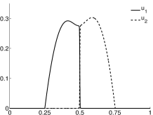
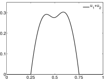
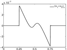
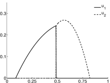
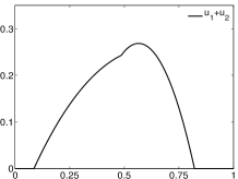
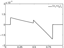
Figure 1: A transient state of solutions of Experiments 1 (first row) and 2 (second row). Left panel: solutions $(u_{1}^{(\delta)},u_{2}^{(\delta)})$. Center panel: The sum $u^{(\delta)}=u_{1}^{(\delta)}+u_{2}^{(\delta)}$. Right panel: the space derivative of the sum, $u_{x}^{(\delta)}$.

In the following experiments we take a uniform partition of $\Omega=(0,1)$ in $10^{3}$ subintervals and the time step $\tau=10^{-5}$. The drift and the linear diffusion coefficients are $b_{i}=c_{i}=0$, and the Lotka-Volterra terms, i.e. the right-hand side of (55) have the form $f_{i}(u_{1},u_{2})=u_{i}(\alpha_{i}-\beta_{i1}u_{1}-\beta_{i2}u_{2})$ with $\alpha_{1}=1,\leavevmode\nobreak\ \beta_{11}=1,\leavevmode\nobreak\ \beta_{12}=0.5,\leavevmode\nobreak\ \alpha_{2}=5,\leavevmode\nobreak\ \beta_{21}=1$,and $\beta_{22}=2$. For the initial data we take $u_{i0}=\exp((x-x_{i})^{2}/0.001)$, $f_{i}=0$ for $i=1,2$ with $x_{1}=0.4$ and $x_{2}=0.6$. Although the initial data do not satisfy the condition $u_{10}+u_{20}>0$ in $\Omega$, this does not seem to affect the convergence or stability of the algorithm for the cases under study. Finally, the tolerance parameter for the fixed point algorithm is set to $\text{tol}=10^{-4}$, and the perturbation parameter to $\delta=10^{-3}$.

We run two experiments according to different nonlinear diffusion matrices. In the first experiment, we set the same diffusion coefficient $a=1$ for both equations, which is the situation studied in Theorems 6.1 and 6.2. In the second experiment we take different diffusivities, $a_{1}=1$ and $a_{2}=3$, in the equations for $u_{1}$ and $u_{2}$ (see (55)). The aim of these experiments is to confirm numerically that, unlike the case of equal diffusivities, in our case the gradient of the sum $u_{1}+u_{2}$ may develop discontinuity. This property can be checked on Figure 1. In the first row we show the results for a transient state of the equal-diffusivities case. Although the independent components of the solution, $u_{1}$ and $u_{2}$ exhibit a discontinuity at the contact point, $x=0.5$, the sum $u_{1}+u_{2}$ is continuous and, as it can be seen in the right panel of the first row, the derivative seems to be continuous as well. In the second row of Figure 1 we show the results corresponding to the different diffusivities case. The behavior is clearly different. Although the continuity of $u_{1}+u_{2}$ still holds, a discontinuity of $(u_{1}+u_{2})_{x}$ at the contact point may be observed.

References

- [1] L. Ambrosio, Transport equation and Cauchy problem for BV vector fields, Invent. math. 158 (2004), 227–260.
- [2] M. Bertsch, M. E. Gurtin, D. Hilhorst, L. A. Peletier, On interacting populations that disperse to avoid crowding: preservation of segregation, J. Math. Biol. 23 (1985) 1–13
- [3] M.Bertsch, R.Dal Passo, M.Mimura A free boundary problem arising in a simplified tumour growth model of contact inhibition, Interfaces and Free Boundaries, 12 (2010) pp. 235–250.
- [4] M. Bertsch, D. Hilhorst, H. Izuhara, M. Mimura, A nonlinear parabolic-hyperbolic system for contact inhibition of cell-growth, Diff. Equ. Appl. 4 (2012) 137–157.
- [5] S. N. Busenberg, C. C. Travis, Epidemic models with spatial spread due to population migration, J. Math. Biol. 16 (1983) 181–198.
- [6] M. A. J. Chaplain, L. Graziano, L. Preziosi, Mathematical modelling of the loss of tissue compression responsiveness and its role in solid tumour development, Math. Med. Biol. 23(3) (2006) 197–229.
- [7] J.I.Díaz, S.Shmarev, Lagrangian approach to the study of level sets: application to a free boundary problem in climatology. Arch. Ration. Mech. Anal. 194 (2009), no. 1, 75–103.
- [8] J.I.Díaz, S.Shmarev, Lagrangian approach to the study of level sets. II. A quasilinear equation in climatology. J. Math. Anal. Appl. 352 (2009), no. 1, 475–495.
- [9] R. J. DiPerna, P. L. Lions, Ordinary differential equations, transport theory and Sobolev spaces, Invent. math. 98 (1989), 511–547.
- [10] G.-Q.Chen, H.Frid. Divergence-measure fields and hyperbolic conservation laws. Arch. Ration. Mech. Anal. 147 (1999), no. 2, 89–118.
- [11] G. Galiano, On a cross-diffusion population model deduced from mutation and splitting of a single species, Comput. Math. Appl. 64(6) (2012) 1927-1936.
- [12] G. Galiano, M. L. Garzón, A. Jüngel, Semi-discretization in time and numerical convergence of solutions of a nonlinear cross-diffusion population model, Numer. Math. 93(4) (2003) 655–673.
- [13] G. Galiano, V. Selgas, On a cross-diffusion segregation problem arising from a model of interacting particles. To appear in Nonlinear Anal. Real World Appl.
- [14] P.Grisvard, Elliptic problems in nonsmooth domains. Monographs and Studies in Mathematics, 24. Pitman (Advanced Publishing Program), Boston, MA, 1985. xiv+410 pp.
- [15] W. S. C. Gurtin, R. M. Nisbet, The regulation of inhommogeneous populations, J. Theor. Biol. 52 (1975) 441–457.
- [16] M. E. Gurtin, A. C. Pipkin, On interacting populations that disperse to avoid crowding, Q. Appl. Math. 42 (1984) 87–94.
- [17] A.Kolmogorov, S.Fomin. Elements of the theory of functions and functional analysis. Vol. 2: Measure. The Lebesgue integral. Hilbert space. Translated from the first (1960) Russian ed. by Hyman Kamel and Horace Komm Graylock Press, Albany, N.Y. 1961 ix+128 pp.
- [18] O. A. Ladyzhenskaya, V. A. Solonnikov, N. N. Ural’ceva Quasillinear Equations of Parabolic Type, Translations of Mathematical Monographs 23, American Mathematical Society, Providence, 1968.
- [19] O.Ladyzhenskaya, N.Ural’tseva, Linear and quasilinear elliptic equations. Translated from the Russian by Scripta Technica, Inc. Translation editor: Leon Ehrenpreis Academic Press, New York-London 1968 xviii+495 pp.
- [20] N. Shigesada, K. Kawasaki, E. Teramoto, Spatial segregation of interacting species, J. Theor. Biol. 79 (1979) 83–99.
- [21] S.Shmarev, Interfaces in solutions of diffusion-absorption equations in arbitrary space dimension. Trends in partial differential equations of mathematical physics, 257–273, Progr. Nonlinear Differential Equations Appl., 61, Birkhäuser, Basel, 2005.
- [22] S.Shmarev, Interfaces in multidimensional diffusion equations with absorption terms. Nonlinear Anal. 53 (2003), no. 6, 791–828.
- [23] S.Shmarev, J.L.Vazquez, The regularity of solutions of reaction-diffusion equations via Lagrangian coordinates. NoDEA Nonlinear Differential Equations Appl. 3 (1996), no. 4, 465–497.