Chaos and dynamical trends in barred galaxies: bridging the gap between $N$-body simulations and time-dependent analytical models

Abstract

Self-consistent $N$-body simulations are efficient tools to study galactic dynamics. However, using them to study individual trajectories (or ensembles) in detail can be challenging. Such orbital studies are important to shed light on global phase space properties, which are the underlying cause of observed structures. The potentials needed to describe self-consistent models are time-dependent. Here, we aim to investigate dynamical properties (regular/chaotic motion) of a non-autonomous galactic system, whose time-dependent potential adequately mimics certain realistic trends arising from $N$-body barred galaxy simulations. We construct a fully time-dependent analytical potential, modeling the gravitational potentials of disc, bar and dark matter halo, whose time-dependent parameters are derived from a simulation. We study the dynamical stability of its reduced time-independent 2-degrees of freedom model, charting the different islands of stability associated with certain orbital morphologies and detecting the chaotic and regular regions. In the full 3-degrees of freedom time-dependent case, we show representative trajectories experiencing typical dynamical behaviours, i.e., interplay between regular and chaotic motion for different epochs. Finally, we study its underlying global dynamical transitions, estimating fractions of (un)stable motion of an ensemble of initial conditions taken from the simulation. For such an ensemble, the fraction of regular motion increases with time.

1 Introduction

Orbits are the fundamental building blocks of any galactic structure and their properties give important insight for understanding the formation and evolution of such structures (Binney & Tremaine, 1987). Our understanding relies significantly on the adequacy and efficiency of the models used either in the time-dependent (TD) self-consistent models or in the rather ‘simpler’ analytical time-independent (TI) ones. The presence of chaos, manifested as unstable orbital motion, and expressed by exponential divergence of nearby trajectories, is broadly studied over the past years (for a good review on chaos in galaxies, see the book by Contopoulos, 2002). It is by now well accepted that the chaotic or regular nature of orbits influences the general stability of the $N$-body simulations, which is straightforwardly related to the underlying dynamics. Therefore, studying the general stability and the detailed structure of the phase (but also of the configuration) space of analytical models can be proven to be very useful, provided that these potentials are realistic in terms of representing density distribution profiles close to those derived by simulations.

The general nature of an orbit, in conservative (TI) systems, can only be one of the following: periodic (stable or unstable), quasi-periodic or chaotic (Lichtenberg & Lieberman, 1992). Nevertheless, there are cases where chaos can be characterized as weak, suggesting that orbits spend a significant fraction of their time in confined regimes and do not fill up phase space as ‘homogeneously’ as the strongly chaotic ones. In these case, the different rate of diffusion in the phase space plays an important role, associated for example the weak chaotic motion with barred or spiral galaxy features, giving rise to a number of interesting results (see e.g. Athanassoula et al., 2009, 2010, 2009; Harsoula & Kalapotharakos, 2009; Harsoula et al., 2011a, b; Contopoulos & Harsoula, 2013; Kaufmann & Contopoulos, 1996; Patsis et al., 1997; Patsis, 2006; Romero-Gómez et al., 2006, 2007; Tsoutsis et al., 2009; Brunetti et al., 2011; Bountis et al., 2012). There are also several results in the recent literature showing that strong local instability does not necessarily imply widespread diffusion in phase space (Cachucho et al., 2010; Giordano & Cincotta, 2004). In Contopoulos & Harsoula (2008, 2010) ‘stickiness’ was studied thoroughly in 2-degrees of freedom (d.o.f.) while in Katsanikas et al. (2011), Katsanikas & Patsis (2011), Katsanikas et al. (2011) and in Manos et al. (2012) the role of ‘sticky’ chaotic orbits and the diffusive behavior, in the neighborhood of invariant tori surrounding periodic solutions of the Hamiltonian in the vicinity of periodic orbits in conservative systems, was also studied.

Doubtless, the different rate of diffusion consists in a very important topic when studying chaotic motion in galactic systems. However, in this paper we mainly focus and concentrate on more general dynamical (in)stability trends using rather standard chaos detection techniques. Over the last years, many chaos detection methods have been developed and also compared, exploiting, in general, either the tangent dynamics of an orbit under study via the simultaneous evolution of its deviation vectors or the analysis of time series constructed by its coordinates. A complete list of all these techniques can be found, e.g. in Contopoulos (2002), in a review paper (Skokos, 2010) and more recently in Maffione et al. (2011, 2013) and references therein. Their efficiency and accuracy on the distinction between regular and chaotic motion has been thoroughly studied and discussed therein as well.

Recently, in Manos et al. (2013), a study was carried out focusing on the dynamics of a barred galaxy model containing a disc and a bulge component. Considering a TD analytical model – extending a TI one (Manos & Athanassoula, 2011) – whose mass parameters of the bar and disc potential vary linearly as functions of time (the one at expense of the other). Two very general conceivable cases in barred galaxies were analyzed: (a) a model where the mass of bar grows, considering a common trend found in $N$-body simulations due to the exchange of angular momentum (see e.g. Athanassoula & Misiriotis, 2002; Athanassoula, 2003) and (b) a case where the bar gets weaker by losing mass (see e.g. Combes, 2008, 2011). There, a new reliable way of using the Generalized Alignment Index (GALI) chaos detection method was used for estimating the relative fraction of chaotic vs. regular orbits in such TD potentials. We stress here that in the TD models, individual trajectories may display sudden transitions from regular to chaotic behavior and vice versa during their time evolution and in general the ‘sticky’ behaviour, as discussed in the literature, is less pronounced. This is also the typical case in the $N$-body simulations where, generally speaking, the motion may also be either: (i) regular throughout the whole evolution, (ii) chaotic throughout the whole evolution, (iii) alternate between chaotic and regular motion with simultaneously orbital shape change (but not necessarily), e.g. from disc to bar like, etc…

Completing furthermore the picture on previous studies on the study of (ir)regular motion in TD systems proposed for cosmological and galactic models, we could refer to a number of publications starting with the definition of the orbital complexity $n(k)$ of an orbital segment which corresponds to the number of frequencies in its discrete Fourier spectrum that contain a $k$-fraction of its total power, used by Kandrup et al. (1997); Siopis et al. (1998). The quantity $n(k)$ was later associated with the short-time evolution of the Lyapunov Exponents (LEs) for TD models in (Siopis et al., 1998). A study in a cosmological system where trajectories were changing their dynamical nature (from regular to chaotic and/or vice-versa) was performed by Kandrup & Drury (1998). The role of friction, noise, periodic driving, black holes was studied by Siopis & Kandrup (2000) while later on this was extended (in Kandrup et al., 2003; Terzić & Kandrup, 2004) following the transient chaos due to damped oscillations. In Sideris (2009) an exponential function of time was added to the Hénon-Heiles potential, using the so-called ‘pattern method’ as chaos detection tool and more recently the dynamics of some simple TD galactic models was investigated (in Caranicolas & Papadopoulos, 2003; Zotos, 2012).

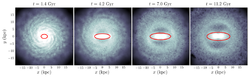
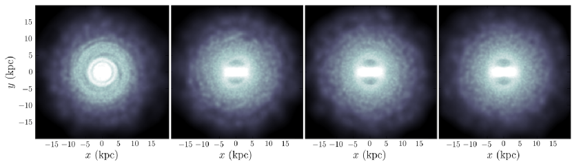
Figure 1: (Colour online) Snapshots of the $N$-body simulation (upper panels) at four different times, displaying stellar density, on the same range, projected on the $xy$ plane. Each frame is 40 by 40 kpc. To illustrate bar lengths and shapes, we overlay ellipses (which are not isophotal fits). Rather, their semi-major axes are obtained from the radial $m=2$ Fourier component of the mass distribution, and from shape measurements via the inertia tensor (see text). The lower panels display the result of evolving an ensemble of initial conditions in the presence of the constructed TD analytical potential.

Regarding the galaxies’ evolution and formation of their several features, it is generally accepted that the most appropriate way to study them is by analyzing $N$-body simulations. The self-consistency of the models in this approach captures much better several details of the general dynamics. The direct application of chaos detection methods to individual orbits is still a rather difficult task while, for a large ensemble of particles, it is even harder if not unfeasible. To overcome this obstacle, mean field potentials have been used in the literature in order to study in more detail the dynamical properties of a specific $N$-body simulation. These potentials are referred to as ‘frozen’ and they are TI and are derived at specific snapshots of the simulations. Hence, one can apply chaos detection tools to the mean field potential instead of the $N$-body simulation. For example, Muzzio et al. (2005) used an elliptical galaxy simulation (no bar or halo) without dissipation which collapses and eventually reaches an equilibrium state. Then, by taking a quadrupolar expansion of the frozen snapshot, they derive a stationary smooth potential. In Voglis et al. (2006) and references therein, the authors deal with disc galaxies, focusing mainly on the spiral structures rather than bars (no halo) while the extraction of the mean field potential is again performed in a similar manner. Following this approach, the role of chaotic motion and diffusion rate in barred spiral galaxies has also been studied (Harsoula & Kalapotharakos, 2009; Harsoula et al., 2011a, b; Maffione et al., 2013; Contopoulos & Harsoula, 2013) while some applications to the Milky Way bar can be found in Wang et al. (2012) and recently a new code for orbit analysis and Schwarzschild modelling of triaxial stellar systems was given in Vasiliev (2013). Nevertheless, following this approach one only derives a stationary mean field model for an equilibrium state of a simulation under study. Furthermore, it does not incorporate an appropriate type set of parameters that would be able to describe and reproduce the time-dependencies in axis ratios, masses, pattern speed, etc. of the several components of a model, like for example the growth of the bar component or the evolution of the disc in time. Let us point out here, the fact that in all these approaches the orbits under study can be only either regular or chaotic. The latter ones may be further distinguished to strongly or weakly chaotic, depending on their diffusion properties, sticky effects etc… during the whole evolution.

In this paper, we consider an $N$-body simulation of a disc galaxy embedded in a live halo (i.e. both the stellar disc and the dark matter halo are represented by responsive particles). Disc-halo interaction leads to the formation of a strong bar. We then measure how the galaxy components vary in time during the simulation. The time evolution of the structural parameters is provided as input to the analytical TD model we build. This ‘candidate’ analytical mean field potential is meant to mimic the $N$-body simulation evolution and more importantly to generate orbits with more similar (and in some sense ‘richer’) morphological behaviour to those of the $N$-body simulation, i.e., permitting for individual orbits the interplay between regular and chaotic epochs as time evolves and providing a stable structure at the same time. Note that, in TI frozen models an orbit cannot convert from chaotic to regular. Our TD model is composed of three components (bar, disc and halo) whose parameters were fitted with the $N$-body measurements, chiefly via the rotation curves. Note that many simplifying assumptions are made. For example, our TD model considers an (ellipsoidal) analytical bar component which is not always an excellent approximation of the shape of the actual $N$-body bar. Likewise, the analytical description of the halo and the disc cannot be expected to behave identically, either. However, our goal is to study the general dynamical impact in stability caused by the bar’s growth in time (as it happens in the $N$-body simulation). Thus, by using a realistic TD model, without aiming to describe of the exact detailed dynamics yielding from the simulation, we can use chaos detection tools and quantify general trends of relative regular and chaos in the phase and configuration space. Keeping this in mind, we draw (disc) initial conditions directly from the simulation and we evolve in time them with the mean field TD potential.

The paper is organized as follows: In Section 2 we describe the $N$-body simulation we used, and we already start presenting the first part of our results, on the construction of a novel time-dependent analytical model and we present its dynamical properties with respect to this simulation. In Section 3 we give briefly the definitions of the chaos detection methods employed and their behaviors for chaotic and regular motion. In Section 4 we explore the global phase space dynamics of the derived analytical model, first for the stationary case (frozen potential), e.g. for different (but fixed) sets of parameters which correspond in a sense to different snapshots of the simulation. In Section 5 we study the dynamical trends and stability of the 3-d.o.f. time-dependent analytical model for both a sample of single orbits but also for a large ensemble of initial conditions from the simulation. Finally, in Section 6 we summarize our findings.

2 $N$-body simulation and construction of the analytical model

Our aim is to construct a time-dependent analytical model that represents the evolution of a barred galaxy. In order to have an astrophysically well motivated model, we supply it with (time-dependent) structural parameters measured from the output of an $N$-body simulation.

2.1 The $N$-body simulation

To serve as the base reference for the analytical model, we use one of the simulations described in Machado & Athanassoula (2010). For simplicity, we select initial conditions with a spherical halo. The mass of the stellar disc is $M_{d}=5\times 10^{10}~{}M_{\odot}$, with an exponential density profile of radial scale length $R_{d}=3.5$ kpc, and vertical scale height $z_{0}=0.7$ kpc:

$$\rho_{d}(R,z)=\frac{M_{d}}{4\pi z_{0}R_{d}^{2}}\exp{\left(-\frac{R}{R_{d}}\right)}\mathrm{sech}^{2}{\left(\frac{z}{z_{0}}\right)},$$ (1)

The spherical dark matter halo has a Hernquist (1993) density profile and it is five times more massive than the disc:

$$\rho_{h}(r)=\frac{M_{h}}{2\pi^{3/2}}\frac{\alpha}{r_{c}}\frac{\exp{(-r^{2}/r_{c}^{2})}}{r^{2}+\gamma^{\prime 2}},$$ (2)

where $M_{h}=2.5\times 10^{11}~{}M_{\odot}$ is the mass of the halo, $\gamma^{\prime}=1.7$ kpc is a core radius and $r_{c}=35$ kpc is a cutoff radius. The normalisation constant $\alpha$ is defined by

$$\alpha=\{1-\sqrt{\pi}q\exp{(q^{2})}[1-\textrm{erf}(q)]\}^{-1}$$ (3)

where $q=\gamma^{\prime}/r_{c}$. For additional details on the initial conditions, see Machado & Athanassoula (2010).

This is a fairly representative collisionless simulation of a strongly barred galaxy. Four snapshots of the disc particles are displayed in the upper row of Fig. 1. It was performed with the $N$-body code gyrfalcon (Dehnen, 2000, 2002) using a total of 1.2 million equal-mass particles, with a gravitational softening length of 0.175 kpc, resulting in 0.1 per cent energy conservation. The simulation was carried out for approximately one Hubble time.

$N$-body simulations have been employed to study chaotic motion in simplified models of disc galaxies. For example, Voglis et al. (2006) study chaos and spiral structure in rotating disc galaxies, but those galaxies are not embedded in dark matter haloes.

The connection between chaos and bars was also analysed by El-Zant & Shlosman (2002), with models were set up by the addition of disc, bar and halo components. They found that in centrally concentrated models, even a mildly triaxial halo lead to the onset of chaos and the dissolution of the bar in a timescale shorter than the Hubble time.

2.2 The time-dependent analytical model

We construct an analytical model that is described by its total gravitational potential $V=V_{B}(t)+V_{D}(t)+V_{H}(t)$, where the three components correspond to the potentials of the bar, disc, and halo, respectively. These components will evolve in time, in accordance with the behaviour we measure from the simulation. Each of these three components is represented in the following way:

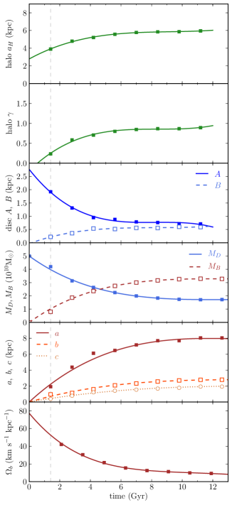
Figure 2: (Colour online) Time evolution of the halo, disc and bar parameters, measured from the $N$-body simulation (points) and supplied to the analytical model (fitted polynomials). First and second panel: parameters of the Dehnen halo profile. Third: parameters of the Miyamoto–Nagai disc. Fourth: bar mass and disc mass. Fifth: semi-major axes of the bar. Sixth: bar pattern speed.

1. A triaxial Ferrers bar (Ferrers, 1877), whose density is given by:

   $$\rho(x,y,z)=\left\{\begin{array}[]{l l}\rho_{c}(1-m^{2})^{2}&\quad\textrm{if}\quad m<1,\\ \quad 0&\quad\textrm{if}\quad m\geq 1,\\ \end{array}\right.$$ (6)

   where $\rho_{c}=\frac{105}{32\pi}\frac{GM_{B}(t)}{abc}$ is the central density, $M_{B}(t)$ is the mass of the bar, which changes in time, and $m^{2}=\frac{x^{2}}{a^{2}}+\frac{y^{2}}{b^{2}}+\frac{z^{2}}{c^{2}}$, $a>b>c>0$, with $a,b$ and $c$ being the semi-axes of the ellipsoidal bar. The corresponding bar potential is:

   $$V_{B}(t)=-\pi Gabc\frac{\rho_{c}}{3}\int_{\lambda}^{\infty}\frac{du}{\Delta(u)}(1-m^{2}(u))^{3},$$ (7)

   where $G$ is the gravitational constant (set to unity), $m^{2}(u)=\frac{x^{2}}{a^{2}+u}+\frac{y^{2}}{b^{2}+u}+\frac{z^{2}}{c^{2}+u}$, $\Delta^{2}(u)=({a^{2}+u})({b^{2}+u})({c^{2}+u})$, and $\lambda$ is the unique positive solution of $m^{2}(\lambda)=1$, outside of the bar ($m\geq 1$), while $\lambda=0$ inside the bar. The analytical expression of the corresponding forces are given in Pfenniger (1984). In our model, the shape parameters (i.e. the lengths of the ellipsoid axes $a$, $b$ and $c$ are) are also functions of time.

2. A disc, represented by the Miyamoto–Nagai potential (Miyamoto & Nagai, 1975):

   $$V_{D}(t)=-\frac{GM_{D}(t)}{\sqrt{x^{2}+y^{2}+(A+\sqrt{z^{2}+B^{2}})^{2}}},$$ (8)

   where $A$ and $B$ are its horizontal and vertical scale-lengths, and $M_{D}(t)$ is the mass of the disc. Here, ‘disc mass’, refers to the stellar mass excluding the bar. As the bar grows, its mass increases at the expense of the remainder of the disc mass, such that the total stellar mass is constant: $M_{B}(t)+M_{D}(t)=5\times 10^{10}~{}M_{\odot}$. The parameters $A$ and $B$ are also functions of time.

3. A spherical dark matter halo, represented by a Dehnen potential (Dehnen, 1993):

   $$V_{H}(t)=\frac{GM_{H}}{a_{H}}\times\left\{\begin{array}[]{lll}-\frac{1}{2-\gamma}\left[1-\left(\frac{r}{r+a_{H}}\right)^{2-\gamma}\right]&,&\hbox{$\gamma\neq 2$,}\\ \ln\frac{r}{r+a_{H}}&,&\hbox{$\gamma=2$.}\end{array}\right.$$ (9)

   $M_{H}$ is the halo mass, $a_{H}$ is a scale radius and the dimensionless parameter $\gamma$ (within $0\leq\gamma<3$) governs the inner slope. The halo mass is constant throughout, but the parameters $a_{H}$ and $\gamma$ are functions of time. For $\gamma<2$ its finite central value is equal to $(2-\gamma)^{-1}GM_{H}/a_{H}$.

Figure 3: (Colour online) Parameters of the Dehnen halo profile and of the Miyamoto–Nagai disc are obtained by fitting the circular velocity curves at each time. Here we display four different times. The fourth column exhibits total, halo and disc circular velocity curves. The first and second columns show the disc density profiles (radial and vertical, respectively). The third column has the halo density profile. Points come from measurements of the $N$-body simulation, while lines are fitted profiles.

Instead of attempting to use the (disc and halo) profiles from the $N$-body simulations, we opted to represent the bar, disc and halo using respectively the Ferrers, Miyamoto–Nagai and Dehnen profiles. There are two reasons for such a choice. First, our approach requires analytical simplicity that could not be afforded by the profiles used in the initial conditions of the numerical simulation. Secondly, due to bar formation and evolution, the initial disc profile in the simulation soon becomes a poor representation in the inner part of the galaxy, where the bar resides. In this sense, it is not advantageous to continue using the initial profiles to model later times. A Miyamoto–Nagai disc provides a sufficient approximation for our purposes. Likewise, even though the Hernquist (1993) halo profile is well suited for numerical purposes, it is inconvenient from the analytical point of view. We experimented with simple logarithmic halo profiles (because their rotation curves are also appropriate), but the Dehnen (1993) profile was preferable, as it provided equally acceptable rotation curves, and a more satisfactory global approximation of the mass distribution. Similarly, fitting the bar by a Ferrers ellipsoid is a justifiable approximation. Surely, it fails to capture the $N$-body bar in all its complexity, particularly after the buckling instability, when the bar is substantially strong and develops the peanut-shaped feature. In general, the $N$-body bar will be more boxy than the Ferrers shape would allow. Nevertheless, fitting an ellipsoid of the same extent allows us to obtain plausible shapes, to determine the bar orientation and to estimate its mass adequately. Ultimately, regardless of small deviations in the density profiles, our goal is to obtain an analytical total potential that is approximately comparable to the overall potential of the simulation.

From the simulation, we are able to measure several quantities as a function of time, which are then used to inform the analytical model.

For the bar, the required parameters are the bar mass, the bar shape and the bar pattern speed $\Omega_{b}$. First, we estimate the bar length as a function of time. This is done by measuring the relative contribution of the $m=2$ Fourier component of the mass distribution as a function of radius, for each time step, and finding the radius at which the $m=2$ has its most intense drop after the peak. This radius $a$ is associated with the bar length. Then we estimate the bar shape by calculating the axis ratios $b/a$ and $c/a$ from the eigenvalues of the inertia tensor in this region. The bar mass is measured by simply adding up the mass enclosed within an ellipsoid of axes $a,b,c$. Finally, the successive orientations of the major axis as a function of time are used to compute the pattern speed. The resulting time evolution of all these quantities are displayed in the fourth, fifth and sixth panels of Fig. 2. Each of these parameters is measured at several time steps, a sample of which is shown, along with the resulting polynomial fits.

The disc mass $M_{D}(t)$ is known once the bar mass has been measured, and the halo mass $M_{H}$ is constant. One still requires the time evolution of two disc parameters ($A$, $B$) and two halo parameters ($a_{H}$, $\gamma$). This is achieved by measuring the rotation curves directly from the simulation (at each time step), and then fitting the analytical $v_{c}(R)$ to these data. Since the disc and halo potentials are known from equations (8) and (9), we obtain their respective analytical circular velocities from $v_{c}^{2}=R\frac{dV}{dR}$:

$$v_{c,D}^{2}(R) = R^{2}~{}\frac{GM_{D}}{\left[R^{2}+(A+B)^{2}\right]^{3/2}}$$ (10)

$$v_{c,H}^{2}(R) = GM_{H}~{}\frac{r^{2-\gamma}}{(r+a_{H})^{3-\gamma}}$$ (11)

Fitting Eq. (11) to the measured halo rotation curve, we obtain $a_{H}$ and $\gamma$. In the case of the disc, it is not enough to fit Eq. (10). One must simultaneously fit the Miyamoto–Nagai density profile to disambiguate the $A+B$ (ignoring the inner part of the disc). When fitting the disc rotation curve, we assume the total stellar mass (i.e. we take both disc and bar mass into account). Since the circular velocities rely on azimuthally averaged quantities, the presence of the bar does not greatly interfere with the quality of the fits, while its removal would lead to spurious results. The measured rotation curves (disc, halo and total), as well as the resulting fitted circular velocities, are displayed in the fourth column of Fig. 3 (at four illustrative instants in time). Errors in the fitted parameters of rotation curves were typically of about 5 per cent or less. Also shown in the first, second and third panels of Fig. 3, are the disc (radial and vertical) and halo density profiles. The points correspond to simulation measurements and the lines give the resulting fits.

One of the main arguments in favor of the adequacy of our analytical model is evidenced by the fact that its total rotation curves are in good agreement with those measured from the simulation. This indicates that the choices of profiles were not unreasonable, as they result in a globally similar gravitational potential. Even if individually the densities of the components are idealized simplifications, the similarity of the total potential ensures that the overall dynamical evolution should be sufficiently well approximated.

Finally, the resulting time evolution of the halo and disc structural parameters, measured in the manner described above, are displayed in the first to fourth panels of Fig. 2. With these, the time-dependence of the analytical model is fully specified. In Table 1 we summarize the analytical model by showing a sample of parameters for the Ferrers bar, Miyamoto–Nagai disc and Dehnen halo potential as fitted by the $N$-body simulation, at four times.

Table 1: The parameters for the Ferrers bar, Miyamoto–Nagai disc and Dehnen halo potential as fitted by the $N$-body simulation, at four times.

				Bar					Disc				Halo
time		$a$	$b$	$c$	$\Omega_{b}$	$M_{B}$		$A$	$B$	$M_{D}$		$a_{H}$	$\gamma$	$M_{H}$
(Gyr)		(kpc)	(kpc)	(kpc)	(km s-1 kpc-1)	($10^{10}M_{\odot}$)		(kpc)	(kpc)	($10^{10}M_{\odot}$)		(kpc)		($10^{10}M_{\odot}$)
1.4		2.24	0.71	0.44	52	1.40		1.92	0.22	3.96		3.90	0.23	25
4.2		5.40	1.76	1.13	24	2.36		0.95	0.53	2.64		5.21	0.71	25
7.0		7.15	2.38	1.58	14	3.02		0.78	0.56	1.98		5.77	0.85	25
11.2		7.98	2.76	1.93	9	3.30		0.71	0.59	1.70		5.95	0.89	25

2.3 Bar strength

In order to measure the bar strengths in analytical models, Manos & Athanassoula (2011) had employed the $Q_{b}$ parameter (Buta et al., 2003, 2004), which is a measure of the relative strength of the non-axisymmetric forces. Here, we opt instead to use a method more familiar to $N$-body simulations, namely measurements of the $m=2$ Fourier component of the mass distribution. For the $N$-body simulation, we measure this component straightforwardly as a function of radius and then take the maximum amplitude to be the $A_{2}$ (see e.g. Athanassoula, Machado & Rodionov, 2013). We refer to this quantity as the bar strength.

For the analytical model, we proceed in a way that allows us to treat it as if it could be represented by particles. We extract from the simulation a random sample of 100 000 initial conditions (i.e. positions and velocities of disc particles) at a time $t_{0}=1.4$ Gyr (see Sect. 5, where we use this ensemble of orbits to further study dynamical trends). The orbits of each of these ‘test particles’ are then evolved forward in time in the presence of our time-dependent analytical potential. Their successive positions can be treated as if they were simulation particles. By stacking them at each time step, we produce the snapshots in the bottom row of Fig. 1. These mock snapshots display a striking resemblance to the $N$-body snapshots, specially bearing in mind that they were obtained by very indirect means. While this comparison cannot be expected to yield a perfect morphological equivalence, one notices that the bar lengths are in quite good agreement, and that in both cases rings are present (although not of the same extent). The point is that the dynamics that arises from the analytical model will give rise to very similar disc and bar morphologies. In fact, the relative importance of the bar is also quite comparable, as indicated by the $A_{2}$ parameter. Analogously to the $N$-body case, we compute the $A_{2}$ of these mock snapshots and compare them in Fig. 4.

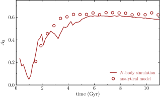
Figure 4: (Colour online) Bar strength, measured from the simulation (line) and from the analytical model (points). $A_{2}$ is the maximum relative contribution of the $m=2$ Fourier component of the mass distribution in the disc.

We must stress here that this comparison is an a posteriori verification, i.e. the bar strength of the $N$-body simulation was in fact not used as an input to the analytical model. The fact the $A_{2}$ do agree well counts as a further sign of the consistency of the constructed analytical model.

It is clear, of course, that the variation of the bar strength modifies the values of several parameters and yields richer information about the dynamics of a self-consistent model. $N$-body simulations show that in general, variations of the bar mass also change the mass ratios of the model’s components, the bar shape and the pattern speed of the galaxy. Hence, if one wishes to use a mean field potential to ‘mimic’ a self-consistent model as accurately as possible, one should allow for all the parameters that describe the bar (together with all other axisymmetric components) to depend on time, assuming that the laws of such dependence were explicitly known. In our case, however, we adopt a simpler approach and vary only the masses of the bar and the disc, as a first step towards investigating such models when time-dependent parameters are taken into account. Thus, we do not pretend to be able to reproduce the exact dynamical evolution of a realistic galactic simulation. Rather, we wish to understand the effects of time dependence on the general features of barred galaxy models and compare the efficiency of chaos indicators like the Generalized ALignment Index (GALI) method and the Maximal Lyapunov Exponent (MLE) in helping us unravel the secrets of the dynamics in such problems.

We stress that the method we introduced to construct the analytical model does not rely – at all – on frozen potentials. Instead, it is grounded on the detailed features of a fully time-dependent, self-consistent $N$-body simulation.

Unless otherwise stated, the units of the analytical model are given as: 1 kpc (length), 1000 km$\cdot$ sec^-1 (velocity), 1 Myr (time), $2\times 10^{11}M_{\bigodot}$ (mass) and km$\cdot$ sec${}^{-1}\cdot$ kpc^-1 ($\Omega_{b}$) while the parameter $G=1$. The total mass $M_{tot}=M_{B}(t)+M_{D}(t)+M_{H}$ is set equal to $3\times 10^{11}M_{\bigodot}$ and since the halo’s mass $M_{H}$ is kept constant, the disc’s mass $M_{D}(t)$ is varied as $M_{D}(t)=M_{tot}-(M_{H}+M_{B}(t))$.

3 Chaos detection techniques

Let us here, for the sake of completeness, briefly recall how the two main chaos detection methods used throughout the paper, namely the GALI and the MLE, are defined and calculated. Considering the following TD 3-d.o.f. Hamiltonian function which determines the motion of a star in a 3 dimensional rotating barred galaxy:

$$H=\frac{1}{2}(p_{x}^{2}+p_{y}^{2}+p_{z}^{2})+V(x,y,z,t)-\Omega_{b}(t)(xp_{y}-yp_{x}).$$ (12)

The bar rotates around its $z$–axis (short axis), while the $x$ direction is along the major axis and the $y$ along the intermediate axis of the bar. The $p_{x}$, $p_{y}$ and $p_{z}$ are the canonically conjugate momenta, $V$ is the potential, $\Omega_{b}(t)$ represents the pattern speed of the bar and $H$ is the total energy of the orbit in the rotating frame of reference (equal to the Jacobi constant in the TI case).

The corresponding equations of motion are:

$$\begin{array}[]{lcl}\dot{x}&=&\displaystyle p_{x}+\Omega_{b}(t)y,\\ \dot{y}&=&\displaystyle p_{y}-\Omega_{b}(t)x,\\ \dot{z}&=&\displaystyle p_{z},\\ \dot{p_{x}}&=&\displaystyle-\frac{\partial V}{\partial x}+\Omega_{b}(t)p_{y},\\ \dot{p_{y}}&=&\displaystyle-\frac{\partial V}{\partial y}-\Omega_{b}(t)p_{x},\\ \dot{p_{z}}&=&\displaystyle-\frac{\partial V}{\partial z},\\ \end{array}$$ (13)

while the equations governing the evolution of a deviation vector $\mathbf{w}=(\delta x,\delta y,\delta z,\delta p_{x},\delta p_{y},\delta p_{z})$ needed for the calculation of the MLE and the GALI, are given by the variational equations:

$$\begin{array}[]{lcl}\dot{\delta x}&=&\displaystyle\delta p_{x}+\Omega_{b}(t)\delta y,\\ \dot{\delta y}&=&\displaystyle\delta p_{y}+\Omega_{b}(t)\delta x,\\ \dot{\delta z}&=&\displaystyle\delta p_{z},\\ \dot{\delta p_{x}}&=&\displaystyle-\frac{\partial^{2}V}{\partial x\partial x}\delta x-\frac{\partial^{2}V}{\partial x\partial y}\delta y-\frac{\partial^{2}V}{\partial x\partial z}\delta z+\Omega_{b}(t)\delta p_{y},\\ \dot{\delta p_{y}}&=&\displaystyle-\frac{\partial^{2}V}{\partial y\partial x}\delta x-\frac{\partial^{2}V}{\partial y\partial y}\delta y-\frac{\partial^{2}V}{\partial y\partial z}\delta z-\Omega_{b}(t)\delta p_{x},\\ \dot{\delta p_{z}}&=&\displaystyle-\frac{\partial^{2}V}{\partial z\partial x}\delta x-\frac{\partial^{2}V}{\partial z\partial y}\delta y-\frac{\partial^{2}V}{\partial z\partial z}\delta z.\\ \end{array}$$ (14)

Regarding the estimation of the value of the MLE, $\lambda_{1}$, of an orbit under study we follow numerically its evolution in time together with its deviation vectors $\mathbf{w}$, by solving the set of equations (13) and (14) respectively. For this task we use a Runge-Kutta method of order 4 with a sufficiently small time step, which guarantees the accuracy of our computations, ensuring the relative errors of the Hamiltonian function (in the TI case) are typically smaller than $10^{-6}$. Furthermore, we need to have a fixed time step in order to ensure that in the TD case the orbits vary simultaneously with the potential.

In general, the derivatives of the potential $V$ depend explicitly on time and and the ordinary differential equations (ODEs) (13) are non-autonomous. Hence, one has to solve together the equations for the deviation vectors (14) with the equations of motion (13). Transforming the Eqs. (13) [and consequently (14)] to an equivalent autonomous system of ODEs by considering time $t$ as an additional coordinate (see e.g. Lichtenberg & Lieberman 1992, section 1.2b), is not particularly helpful, and is better to be avoided as shown in Grygiel & Szlachetka (1995).

So, in order to compute the MLE and the GALI we numerically solve the time-dependent set of ODEs (13) and (14). Then, according to Benettin et al. (1976); Contopoulos et al. (1978); Benettin et al. (1980) the MLE $\lambda_{1}$ is defined as:

$$\lambda_{1}=\lim_{t\rightarrow\infty}\sigma_{1}(t),$$ (15)

where:

$$\sigma_{1}(t)=\frac{1}{t}\ln\frac{\|\mathbf{w}(t)\|}{\|\mathbf{w}(0)\|},$$ (16)

is the so-called ‘finite time MLE’, with $\|\mathbf{w}(0)\|$ and $\|\mathbf{w}(t)\|$ being the Euclidean norm of the deviation vector at times $t=0$ and $t>0$ respectively. A detailed description of the numerical algorithm used for the evaluation of the MLE can be found in Skokos (2010).

This computation can be used to distinguish between regular and chaotic orbits, since $\sigma_{1}(t)$ tends to zero (following a power law $\propto t^{-1}$) in the former case, and converges to a positive value in the latter. But Hamiltonian (Eq. 12) is TD, which means that its orbits could change their dynamical behavior from regular to chaotic and vice versa, over different time intervals of their evolution. In such cases, the MLE (15) does not behave exactly as in TI model (presenting in general stronger fluctuations) and its computation might not be able to identify the various dynamical phases of the orbits, since by definition it characterizes the asymptotic behavior of an orbit (see e.g. Manos et al., 2013). Nevertheless, we will show the MLE for a number of orbits throughout the paper, for a more global discussion of the several dynamical properties observed.

Thus, in order to avoid such problems in our study, we use the GALI method of chaos detection (Skokos et al., 2007). The GALI index of order $k$ (GALI_k) is determined through the evolution of $2\leq k\leq N$ initially linearly independent deviation vectors $\textbf{w}_{i}(0)$, $i=1,2,\ldots,k$, with $N$ denoting the dimensionality of the phase space of our system. Thus, apart from solving Eqs. (13), which determines the evolution of an orbit, we have to simultaneously solve Eqs. (14) for each one of the $k$ deviation vectors. Then, according to Skokos et al. (2007), GALI_k is defined as the volume of the $k$-parallelogram having as edges the $k$ unit deviation vectors $\hat{\textbf{w}}_{i}(t)=\textbf{w}_{i}(t)/\|\textbf{w}_{i}(t)\|$, $i=1,2,...,k$. It can be shown, that this volume is equal to the norm of the wedge product (denoted by $\wedge$) of these vectors:

$$\textrm{GALI}_{k}(t)=\parallel\hat{\textbf{w}}_{1}(t)\wedge\hat{\textbf{w}}_{2}(t)\wedge\ldots\wedge\hat{\textbf{w}}_{p}(t)\parallel.$$ (17)

We note that in the above equation the $k$ deviation vectors are normalized but their directions are kept intact.

In principal and for TI systems, the GALI${}_{k}(t)$ for regular orbits remains practically constant and positive if $k$ is smaller or equal to the dimensionality of the torus on which the motion occurs, otherwise, it decreases to zero following a power law decay. For the chaotic ones, all GALI${}_{k}(t)$ tend exponentially to zero with exponents that depend on the first $k$ LEs of the orbit (Skokos et al., 2007, 2008). Nevertheless, in the TD case studied in Manos et al. (2013) and also here, the way the theoretical estimation of the GALI’s exponential rates are strongly related to the LEs, being more complicated and still open to further inquiry.

The procedure used for the detection of the several different dynamical epochs of the TD system is the following: We evolve the GALI_k with $k=2$ or $k=3$ (i.e., using 2 or 3 deviation vectors) for the 2-d.o.f or 3-d.o.f. cases respectively and whenever GALI_k reaches very small values (i.e. GALI${}_{k}\leq 10^{-8}$) we re-initialize its computation by taking again $k$ new random orthonormal deviation vectors, which resets the GALI${}_{k}=1$. We allow then these vectors to evolve under the current dynamics. For time intervals where the index decays exponentially corresponds to chaotic epochs while in the other cases to non-chaotic. The reason in doing this is that we need to follow the current dynamical stability of an orbit under-study which in principle can interplay between chaotic and regular for different epochs during the total time evolution. Thus, let us assume that a trajectory experiences chaotic dynamics and later on drifts to a regular regime. The volume formed by the deviation vectors will first shrink exponentially to very small values and remain small throughout the whole evolution unless one re-initializes the deviation vectors and their volume, in order to allow them to ‘feel’ the new current dynamics. However, when we are interested in more general dynamical trends in time (less details), we will fix time intervals and we will re-initialize the deviation vectors in the beginning of each one.

4 The 2-d.o.f. time-independent case

Shedding some light on the underlying TI dynamics is an important step for understanding the more complicated case of the fully 3-d.o.f. TD model where all parameters vary simultaneously in time.

By setting $z,p_{z}$ equal to zero at $t=0$ (remaining zero at all times) in the Hamiltonian Eq. (12), the orbits’ motion is then restricted in the 2 dimensional $(x,y)$ space. Note that here $t=0$ refers to the $t_{0}=1.4$ Gyr of the $N$-body simulation. We can then study, in a frozen potential, individual orbits and the stability of the phase space, in terms of detecting and locating chaotic and regular motion, for the several sets of the potential parameters at deferent times, as derived from the $N$-body simulation. We shall begin by choosing fixed parameters from four time snapshots, i.e., at $t=1.4$ Gyr, $t=4.2$ Gyr, $t=7.0$ Gyr and $t=11.2$ Gyr and we integrate orbits for 10 Gyr.

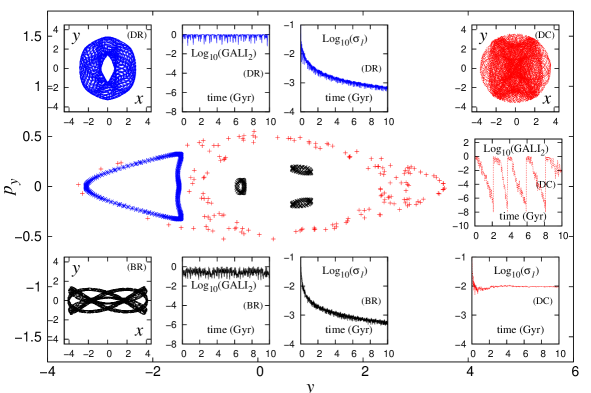
Figure 5: (Colour online) The Poincaré Surface of Section defined by $x=0$, $p_{x}\geq 0$ with $H=-0.19$, for three typical orbits (two regular and one chaotic) being integrated for 10 Gyr. The set of parameters for the bar, disc and halo components are chosen from the fits with the 3-d.o.f. TD Hamiltonian at $t=7.0$ Gyr of the $N$-body simulation. In the insets we depict their projection on the $(x,y)$-plane together with the GALI₂ and MLE $\sigma_{1}$ evolution in time (see Table 1 for the exact parameters and text for more details on these trajectories).

In Fig. 5, we present the Poincaré Surface of Section (PSS) defined by $x=0$, $p_{x}\geq 0$ with $H=-0.19$, for three typical orbits being integrated for 10 Gyr. The set of parameters for the bar, disc and halo components are chosen from the fits with the 3-d.o.f. TD Hamiltonian at $t=7.0$ Gyr of the $N$-body simulation (see Table 1 for more details). The blue $(\ast)$ points on the PSS correspond to a disc regular orbit, forming a curve by the successive intersections with the plane $x=0$, having initial condition $(y,p_{y})=(-1.5,0.0)$ with $x=0$ and $p_{x}=H(x,y,p_{y})$ (called ‘DR’ from now on). Its projection on the $(x,y)$-plane is shown in the top left inset panels of Fig. 5 and coloured in blue. The GALI₂ for this orbit confirms that its motion is regular by oscillating to a positive value during its evolution in time as well as the MLE $\sigma_{1}$ following a power law decay [see second and third top inset panels of Fig. 5 respectively (blue), note that the axis here are in lin-log scale]. The three small black curves in the central part of Fig. 5, marked with ($\times$), are formed by the successive intersections of an initial condition with $(y,p_{y})=(-0.4,0.0)$ (we will call it ‘BR’). From its projection on the $(x,y)$-plane [first bottom inset panel of Fig. 5 (black)], it is evident that it is a bar-like orbit elongated along the long $x$-axis. It surrounds a stable periodic orbit of period 3 in the center of these islands and its regular dynamics is clearly revealed from the evolution of the GALI₂ and the MLE $\sigma_{1}$ evolution [second and third top (black) inset panels of Fig. 5 respectively, note that the axis are again in lin-log scale]. The central scattered red points on the PSS, marked with $(+)$, correspond to a chaotic orbit with initial condition $(y,p_{y})=(2.5,0.0)$ (called ‘DC’ from now on). In the three inset panels positioned vertically in the right part of the Fig. 5 (red), we depict its projection on the $(x,y)$-plane (top panel). Its GALI₂ successive and exponential decrease to zero in time (middle panel) indicates its chaotic nature. Notice that we re-initialize the deviation vectors each time the index becomes small $(\leq 10^{-8})$. Its MLE $\sigma_{1}$, as expected, converges to a positive value (bottom inset).

Since in this case, the potential has no TD parameters, the general asymptotic nature can be either regular or chaotic (weakly or strongly). This of course will change when the parameters start to vary in time and the motion can convert from one kind to the other, though this will be driven by the momentary underlying dynamics. Hence, it is important to have a good idea of how the phase space (through the potential parameters) evolves in time and for different values of the Hamiltonian function. Regarding the former we will pick four sets of parameters given at different times as extracted from the $N$-body simulation, i.e., at $t=1.4$ Gyr when the bar is still relatively small, at the end of the simulation ($t=11.2$ Gyr) and at two intermediate states ($t=4.2$ Gyr and $t=7.0$ Gyr). The next step is to pick some ‘representative’ or ‘most significant’ energy (Hamiltonian function) values from the total available energy spectrum at each time and set of parameters that would be relevant for the $N$-body simulation as well. For this reason, we first calculated the energy dispersion of the 100 000 disc particles from the simulation. The energies are calculated from the TD Hamiltonian function Eq. (12) at $t_{0}=1.4$ Gyr. In the inset panel we show the cumulative distribution of this set of orbits. From the energy distribution histogram in Fig. 6,

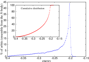
Figure 6: (Colour online) Dispersion energy histogram for an ensemble of 100 000 initial conditions from the $N$-body simulation. The energies are calculated from the TD Hamiltonian function Eq. (12) at $t_{0}=1.4$ Gyr. In the inset panel we show the cumulative distribution of this set of orbits.

we can see that the majority of the trajectories of the $N$-body simulation are concentrated in relatively large values.

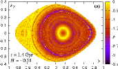
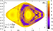
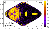
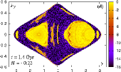
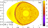
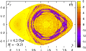
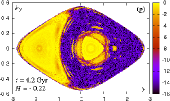
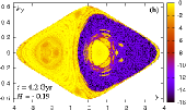
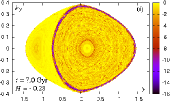
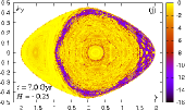
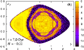
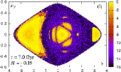
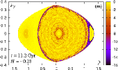
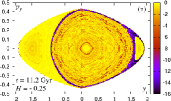
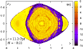
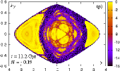
Figure 7: (Colour online) The (in)stability map for the 2-d.o.f. frozen potential case using a grid of $\approx$ 100 000 initial conditions on the PSS and integrating them for 10 Gyr. The colour-bar represents the final GALI₂ values of each initial condition in the end of the iteration. The first row refers to a set of potential parameter given at $t=1.4$ Gyr for Hamiltonian values $H=-0.31,-0.28,-0.25,-0.22$, the second row at $t=4.2$ Gyr for $H=-0.28,-0.25,-0.22,-0.19$, the third row at $t=7.0$ Gyr for $H=-0.28,-0.25,-0.22,-0.19$ and the fourth row at $t=11.2$ Gyr for $H=-0.28,-0.25,-0.22,-0.19$. The yellow (light-grey in b/w) colour corresponds to regular orbits where the GALI₂ oscillates around to relatively large positive values, the black color represents the chaotic orbits where GALI₂ tends exponentially small values, while the intermediate colors in the colour-bars between the two represent ‘weakly chaotic or sticky’ orbits. The exact set of parameters used at each $t=1.4,4.2,7.0,11.2$ Gyr are given in table 1.

Exploiting this information, we first choose a sample of 2-d.o.f. Hamiltonian function values (for the four times mentioned above and the respective sets of parameters), from the interval of energies where the majority of the $N$-body simulation’s particles is more probable to be found. From this sample, we select a subset of representative energies to illustrate typical phase space structures, focusing at this point on the underlying dynamics. Then, we chart the regular and chaotic regimes of the phase space with GALI₂. In Fig. 7, we have used a grid of 100 000 initial conditions on the $(y,p_{y})$-plane of the corresponding PSS and we have constructed a (colour online) chart of the chaotic and regular regions similar to the PSS, but with more accuracy and higher resolution, in a similar manner just like in Manos & Athanassoula (2011), using the GALI₂ method. The different colour corresponds to the different final value of the GALI₂ after 10 Gyr (10 000 time units) for orbits representing each cell of the grid. The yellow (light-grey in b/w) colour corresponds to regular orbits (and areas) where the GALI₂ oscillates around to relatively large positive values, the black color represents the chaotic orbits where GALI₂ tends exponentially to zero (10^-16), while the intermediate colors in the colour-bars between the two represent ‘weakly chaotic or sticky’ orbits, i.e. orbits that ‘stick’ onto quasi-periodic tori for long times but their nature is eventually revealed to be chaotic. Note that the model in this case is TI and hence there is no need for re-initialization of the deviation vectors, since the asymptotic dynamical nature of the orbits does not change in time. The first row refers to a set of potential parameter given at $t=1.4$ Gyr for Hamiltonian values $H=-0.31,-0.28,-0.25,-0.22$, the second row at $t=4.2$ Gyr for $H=-0.28,-0.25,-0.22,-0.19$, the third row at $t=7.0$ Gyr for $H=-0.28,-0.25,-0.22,-0.19$ and the fourth row at $t=11.2$ Gyr for $H=-0.28,-0.25,-0.22,-0.19$.

Using the above approach, we can measure and quantify the variation of the percentage of regular orbits in the phase space as the total energy increases for a specific choice of potential parameters at same fixed times. The chosen values of the Hamiltonian functions cover the range of the available energy interval up to the value of the escape energy which in general is different. Although the main general trend is that this percentage decreases as the energy grows, its behavior changes at high energy values where it is no more monotonic. Note that this happens for energy values $H>-0.19$ out of the range of $N$-body simulation orbits. In Fig. 8 we show the variation of percentages of regular motion as a function of the energy $H$ for the different sets of parameters at $t=1.4$ Gyr, $t=4.2$ Gyr, $t=7.0$ Gyr and $t=11.2$ Gyr. The threshold GALI${}_{2}\geq 10^{-8}$ was used to characterize an orbit as regular and GALI${}_{2}<10^{-8}$ as chaotic which will also be the chaos criterion/threshold throughout this paper. We should emphasize that these percentages refer to a set of initial conditions that cover uniformly the whole 2-d.o.f. phase space. On the other hand, an ensemble of trajectories extracted from the $N$-body simulation does not necessarily populate ‘democratically’ the phase space. By simply inspecting these percentages one can claim that the fraction of regular motion is systematically larger for later times, and for all energies. When looking and comparing the phase space for early times, i.e., $t=1.4,4.2$ Gyr (first and second row) and late times, i.e., $t=7.0,11.2$ Gyr (third and fourth row) in Fig. 7, we may see that the central island of stability, originating bar-like orbits, is becoming larger as the time grows and this is even more evident for the relatively larger energies (see the third and fourth row from top to bottom). This indicates that the bar component becomes gradually more important and dominant.

Considering the $N$-body simulation’s bar growth evolution (Fig. 1), this fact seems to be already in a quite good agreement, since one would expect the barred morphological features to become more evident as time increases and for the relevant energies, in both the simulation and the derived TD analytical model. We may here note that the energies of the $N$-body simulation particles (being 3 dimensional objects) are concentrated in the interval $-0.3\lesssim H\lesssim-0.2$ (as shown in Fig. 6). A more ‘realistic’ ensemble of initial conditions will be used for the 3-d.o.f. case in the next section. Despite the fact that these percentages refer to the 2-d.o.f. case, one may get a brief idea of how the relative stability of the phase space changes as the energy varies in the ‘full’ 3-d.o.f. model and expect a relatively large fraction of regular motion for an ensemble chosen within this energy interval.

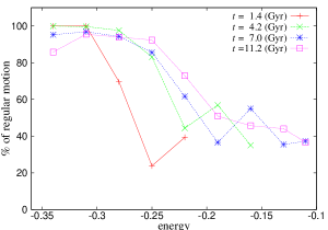
Figure 8: (Colour online) Percentages of regular motion for the 2-d.o.f. frozen case as a function of the energy $H$ for the different sets of parameters at $t=1.4$ Gyr, $t=4.2$ Gyr, $t=7.0$ Gyr and $t=11.2$ Gyr.

5 The 3-d.o.f. time-dependent model

For the global study of the dynamics of the phase and configuration space of a 3-d.o.f. model (TI and/or TD), the choice of initial conditions plays a crucial role. When one seeks to explore the whole available phase space the orbits might occupy, a few useful approaches have been proposed and used in the literature (e.g. Schwarzschild, 1993; Papaphilippou & Laskar, 1998; El-Zant & Shlosman, 2002), where some adequate (but different) ways in populating several different families of orbits were proposed by giving initial conditions on several appropriate chosen planes in positions and momenta with the total energy restriction taken into account (also used recently in Maffione et al., 2013). In Manos & Athanassoula (2011) and Manos et al. (2013) the authors used two similar distributions as in the latter references and also a third one, derived by a random set of orbits related to the density mass distribution of the model. Their momenta were set zero along the $y,z$ directions while the $p_{x}$ was estimated by the total Hamiltonian function value, randomly chosen from the available energy level. The approaches described above may supplementary explore well the phase space of a model. However, they do not ensure that the particles of a realistic $N$-Body simulation necessarily populate the phase space in the same uniform way. This becomes even more complicated when the potential under consideration ceases to be TI and the parameters’ time-dependencies in time cause consecutive alternations in the phase space.

For these reasons, here, and in order to study global stability and dynamical trends in our 3-d.o.f. TD analytical model, we extract an ensemble of 100 000 initial conditions directly from the $N$-body simulation at the time $t_{0}=1.4$ Gyr where the bar has already started to be formed and starts growing from that point on. Note that these orbits are chosen only from the disc density distribution of the simulation and do not include halo particles. Our goal is twofold: (i) to estimate quantitatively the fraction of chaotic and regular motion as time increases and (ii) to check whether and how this variation is associated now to the bar strength for this TD model. From this point and on, we attribute the time $t_{0}=1.4$ Gyr to $t_{0}=0$. Then, in the TD analytical model, the orbits are integrated for $10$ Gyr (a bit less than a Hubble time), a realistic upper limit related to the $N$-body simulation’s set up.

Let us point out here that the straightforward comparison of the two approaches is rather difficult, since several assumptions have been made for the construction of the TD analytical model. For example, the total energy of the particles is not expected to be conserved, like in the $N$-body simulation where the self-consistency ensures this with a good accuracy. Moreover, halo particles, present in the $N$-body simulation, are not taken into account as point mass particles at this point. The reason, as explained earlier, is that we are mainly interested in the bar’s growth and evolution in time. Hence, when one allows all the TD model parameters of the several components of model to vary in time for a set of initial conditions, the total energy is not conserved. Nevertheless, and for the sake of a more general study, we tried two alternative cases; let us call them dynamical scenarios whose parameters are given in such a way that the total energy can be conserved by making reasonable assumptions. We then checked how sensitive the general dynamical trends are to these choices of potentials.

Scenario A:

In this case, all the parameters of the three components (bar-disc-halo) of the potential vary simultaneously in time, following the fitting functions derived from the simulation. In this case the value of the Hamiltonian in general is not conserved in time for a single trajectory. Here, the TD model incorporates the time-dependencies of the $N$-body simulation for each particle, however in the latter the sum of the energy of all the particles remains approximately constant. This is the evolutionary scenario presented in the panels of the lower row in Fig. 1. We can see that this TD model can capture quite successfully the basic trends and the bar formation of the $N$-body simulation (upper row).

Scenario B:

In this case, the parameters of the bar and disc vary as in case ‘Scenario A’ but the halo ones are adjusted in such a way that the value of the total Hamiltonian function, for each initial condition, remains constant in time. In order to achieve that, we first allow the bar and disc potential to vary in time as before, keeping constant the halo parameter $\gamma$ ($\approx 0.234$ at $t_{0}=1.4$ Gyr) and then we allow the $a_{H}$ to vary at each time step. From the initially known Hamiltonian value, we calculate the value of the total potential at every time step and then find the value of the $V_{H}(t)$ such as the total energy remains constant. Having this value, we can numerically estimate the appropriate value of $a_{H}(t)$ that fulfills the imposed energy conservation condition. This also implies that the scale radius of the halo might vary in a similar way for all the orbits but not identically so.

Scenario C:

In this case, the bar parameters are completely time-dependent, the disc parameters are fixed in an approximately averaged value, with respect to the whole evolution, i.e., $A=0.8$ and $B=0.55$, while the halo parameters are estimated just like in case ‘Scenario B’, obtaining again the energy conservation.

Before focusing on the general dynamical trends of the above different scenarios, let us first study the evolution of a few typical examples of orbits. We picked a random but representative (in terms of radial distance) number of orbits from our 100 000 initial conditions and calculated their orbital evolution together with their GALI₃ and MLE. Let us mention here that for all three Scenarios the number of escaping orbits is negligible. From this subset of orbits, we chose to show here, in Fig. 9 and Fig. 10, two typical examples of trajectories which present also a rather ‘rich’ and interesting morphological behaviour. Each figure is divided in three main blocks, each one corresponding to the different evolution Scenarios A, B and C respectively. Then, each block is further composed of three parts where the orbital evolution is depicted on the $(x,y)$-plane in the course of time (first rows of each subpart), together with the GALI₃ and MLE $\sigma_{1}$ in the next two rows respectively.

Scenario A (bar-like orbit $B1$)

 

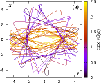
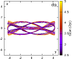
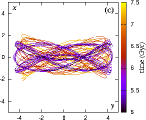
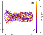
Scenario B (bar-like orbit $B1$)

 

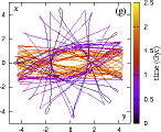
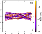
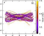
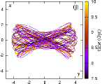
Scenario C (bar-like orbit $B1$)

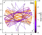
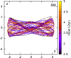
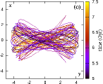
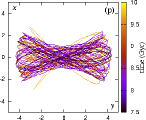
Figure 9: (Colour online) The 3-d.o.f. orbit $B1$ evolved with the Scenario A, B and C. Its different projection on the $(x,y)$-plane in different time windows is depicted in the first (four-panel) row (from top block-part to the bottom respectively) and the colour bar corresponds to the time (in Gyr). Their GALI₃ and MLE $\sigma_{1}$ evolution in time is shown for each case just below them. Note that the orbit (in all three cases) starts as a disc-like and gradually its shape turns to barred, displaying the bar’s growth through the parameters of the Ferrers’ potential (see text for more details).

Scenario A (disc-like orbit $D1$)

 

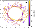
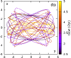
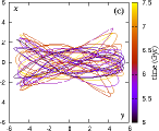
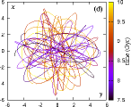
Scenario B (disc-like orbit $D1$)

 

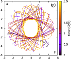
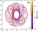
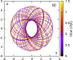
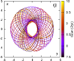
Scenario C (disc-like orbit $D1$)

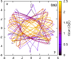
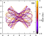
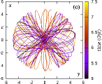
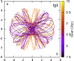
Figure 10: (Colour online) Same as in Fig. 9 but for the 3-d.o.f. disc-like orbit $D2$ evolved again with the ‘Scenario A, B and C’. Note, that here the disc-like pattern slightly varies from cases to case. The different degree of chaoticity can be accurately captured by the frequency and fast decay to zero of the GALI₃ [Fig. 10(e,k,q)], indicating that the orbits is relatively ‘strongly chaotic’ under the ‘Scenario A, C’ while under the ‘Scenario B’ is relatively ‘weakly chaotic’. This information can not be revealed in such a way by the MLE $\sigma_{1}$ shown in Figs. 10(f,l,r) (see text for more information).

Thus, in Fig. 9 we show the evolution of an orbit from the ensemble of the $N$-body simulation with initial condition $(x,y,z,p_{x},p_{y},p_{z})\approx$ $(-4.543100,0.499639,-0.162627,\newline 0.048798,-0.218718,0.002898)$ (we will refer to this orbit from now on as ‘$B1$’), which is iterated for 10 Gyr (10 000 time units) for the TD potentials mentioned above. The $B1$ orbit belongs to a set of initial conditions which is representative of the imposed scenario of the bar growth by our TD potential. The starting and complete set of parameters for the TD model is taken at $t_{0}=1.4$ Gyr by the fits with the $N$-body simulation with the procedure described in Section 2. Note that in all figures’ panels, we set everywhere the $t_{0}$ equal to zero instead of $t_{0}=1.4$ Gyr.

In the first row of the first block in Fig. 9(a,b,c,d), we show its projection on the $(x,y)$-plane for four successive time intervals of $\Delta t=2.5$ Gyr when evolved by the ‘Scenario A’, i.e., all the three potential components $V_{B},V_{D},V_{H}$ are time-dependent and the total energy is not in general conserved. The colour bar next to each panel corresponds to the time (in Gyr), hence the most recent epochs of the orbit are coloured with yellow (light-grey in b/w) while those in the earlier ones with dark blue or black (dark-grey or black in b/w). In Fig. 9(e) we show its GALI₃, capturing accurately the chaotic nature of the orbit during the first [Fig. 9(a)], third [Fig. 9(c)] and fourth [Fig. 9(d)] time windows by decaying exponentially to zero. On the other hand, in the second [Fig. 9(b)] time window its regular (even by just looking its projected morphologically on the $(x,y)$-plane) behaviour is successfully revealed by the fluctuates to a non-zero value of the index. Note that the plot is in lin-log scale and the deviation vectors are re-initialized, by taking again $k$ new random orthonormal deviation vectors, each time the GALI₃ becomes very small (i.e. GALI${}_{3}\leq 10^{-8}$). It turns out that the $B1$ begins as a regular disc-like orbit during the first 2.5 Gyr and, as the bar starts forming and growing, it gradually evolves to a chaotic bar-like orbit until the end of the integration. We may notice how hard it is for the finite time MLE $\sigma_{1}$ [Fig. 9(f)] to capture these different dynamical different transitions and epochs due to its time-averaged definition (see also Manos et al., 2013). Furthermore, its power law decay for regular time intervals and its tendency to positive values for chaotic ones are of the same order of magnitude making it rather hard to use the temporary value $\sigma_{1}$ as a safe criterion of regular and weak or strong chaotic motion.

In order to see how morphologically sensitive our ‘full’ TD parameter model is (as described in ‘Scenario A’) to the several component parameters and the lack of energy conservation, let us evolve the same initial condition ($B1$) with the ‘Scenario B’. We can see that, the general shape of the orbits is more or less similar, starting again as an disc-like orbit and drifting to a bar-like one in time [first row of the second block in Fig. 9(g,h,i,j)]. Of course, the dynamical epochs are a bit different. In the first row of the third block in Fig. 9(m,n,o,p), we show its evolution when integrated with the time-dependencies described in the ‘Scenario C’ and recovering again similar morphological behaviour. In the elongated panels, beneath the projections on the $(x,y)$-place of the ‘Scenario B, C’, we depict their corresponding GALI₃ [Fig. 9(k,q) respectively] and MLE $\sigma_{1}$ [Fig. 9(l,r) respectively] just like for the ‘Scenario A’.

Of course, we should not expect such a good agreement in the several morphological behaviours in general and for all orbits of the initial ensemble. More specifically, and in cases where chaos is strong from the very early moments, the orbits are expected to differ significantly depending on the evolutionary scenario. As also discussed in Carpintero & Wachlin (2006), the chaotic behaviour is sensitive to the choice of the potential, even if it is frozen like in their case.

In Fig. 10, and in a similar manner as in Fig. 9, we show another characteristic disc-like orbit for most of the total of integration with initial condition $(x,y,z,p_{x},p_{y},p_{z})\approx$ $(-5.14416,-1.345540,0.277956,\newline 0.140120,-0.219648,0.000338)$ (we will refer to this orbit from now on as ‘$D1$’). The evolutionary scenarios are again the same as before, i.e., in the first row of the first block in Fig. 10(a,b,c,d), we present its projection on the $(x,y)$-plane for different time windows. The $D1$ orbit experiences a regular epoch during its first 2.5 Gyr, then gradually becomes chaotic switching to a bar-like shape and finally becomes a chaotic but disc-like now orbit. Its regular and chaotic epochs are accurately captured by the GALI₃ [Fig. 10(e)], fluctuating to constant value for the first 2.5 Gyr and then successively decaying exponentially to zero for the rest of the integration. The MLE $\sigma_{1}$ [Fig. 10(f)] also reveals this dynamical evolution, by decaying with a power law for the regular part and converging to non-zero value for the three last time windows. However, here the motion does not present any further transition and/or interplay between regular and chaotic motion and again (as for the $B1$ orbit) the order of magnitude for the $\sigma_{1}$ is not varying sufficiently enough to lead to a safe conclusion at certain times without seeing its whole time evolution.

Its evolution with the ‘Scenario B’, is shown in the first row of second middle block in Fig. 10(g,h,i,j)] where it turns out that presents different morphological shape. In more detail, it still begins similarly but for later times it forms a disc-like orbit (less chaotic also) which does not visit the central region compared to what happens in ‘Scenario A’. Moreover, when looking at its shape when integrated with the ‘Scenario C’ [Fig. 10(m,n,o,p)], we can again conclude that it is a chaotic disc-like orbit but not identical to the other cases. Notice that, the different degree of chaoticity can be accurately captured by the frequency and fast decay to zero of the GALI₃ [Fig. 10(e,k,q)], indicating that the orbits is relatively strongly chaotic under the ‘Scenario A, C’ while under the ‘Scenario B’ is relatively weakly chaotic. This information can not be revealed in such a way by the MLE $\sigma_{1}$ [Fig. 10(f,l,r)].

Furthermore, let us clarify the following for such TD systems. When speaking more strictly and using more rigorous notions from non-linear dynamics theory, those orbits experiencing such an interplay between regular and chaotic epochs in different time intervals are in general (asymptotically) chaotic. Their MLE is positive (like in our examples in Fig. 9 and Fig. 10). However, when one is interested in astronomical time scales, one may split the time in smaller windows and see how an ensemble of orbits evolve. There, one may detect the different orbital trends (general at first), in terms of chaotic or regular by checking the local exponential divergence. The GALI method is one good way to capture these phenomena quite successfully, after giving enough time to the deviation vectors to detect the stability of the local dynamics. Since one cannot know or predict in advance, when exactly such transitions between regular and chaotic motion will occur for each individual trajectory, one is limited to the study of rather average trends.

One common approach broadly performed in the recent literature is to measure the relative fraction of regular and chaotic motion in a sequence of frozen snapshots (e.g. Valluri et al., 2010). However, this would not allow us to capture an important and abundant orbital behaviour in the $N$-body simulations, namely orbits that alternate their nature from regular to chaotic and vice-versa as well as their morphological shape, e.g. from disc-like shape to barred-like one.

Turning now to the aspect of the global (in)stability of the model and this set of initial conditions in particular, one would be interested to monitor the variation of the total fraction of regular vs. chaotic motion in the course of time. Since our model is TD the percentage of chaotic orbits following the potentials (described as Scenarios A, B and C) is expected to change in time. In order to estimate this we adopt the following strategy: We divide the total integration time of 10 Gyr in four successive time windows of length $\Delta t=2.5$ Gyr time units. At the beginning of each time window, we re-initialize GALI₃ to unity and follow a new set of three orthonormal deviation vectors for each orbit. Then for each time window we calculate the current percentage of regular (non-chaotic) orbits as the fraction of orbits whose GALI₃ remains $>10^{-8}$ during that time interval, i.e., GALI₃ does not decay exponentially (fast) to small values. In this way we allow the GALI₃ to have enough evolutionary time to reveal the chaotic or regular nature of the orbit within this interval. The results of this procedure are shown in Fig. 11,

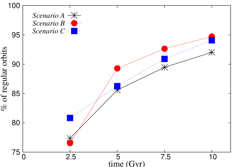
Figure 11: (Colour online) Percentages of regular motion for different time windows.

where we depict the percentages of regular motion for different time windows for the ensembles of initial conditions evolved under the three different evolutionary processes. Though, it turns out that all three dynamical evolutionary cases show quite similar trends, in terms of fraction of chaotic and regular motion, implying that the variations of the halo and disc parameters effect is relatively weak with respect to the bar’s. The amount of regular motion for the three different cases systematically grows in time, starting from $\approx 75\%$ to $\approx 81\%$ after $2.5$ Gyr reaching $\approx 90\%$ to $\approx 94\%$ after $10$ Gyr. The ‘Scenario A’ turns out to be slightly more chaotic compared to other two. Moreover, let us stress the fact that the presence of regular motion is abundant in this TD model when comparing to similar studies (Manos & Athanassoula, 2011; Manos et al., 2013) where chaos turned out to be dominant.

The next step is to see how the bar strength is related to the general (average) stability. As found and discussed in Manos & Athanassoula (2011), and for TI modes, one should expect to find a strong correlation between the strong bars and the total amount of chaos. This result was confirmed for a simple TD model, where only the mass of bar was considered to grow in time in Manos et al. (2013), in a potential also composed of a bar and a disc but of a bulge instead a halo component. By simply looking at the percentages of regular motion in Fig. 11, one would conjecture that the relative non-axisymmetric forcings are decreasing slightly in time, implying that the bar gets weaker.

However, this is not what happens here. As shown in Fig. 4, the $A_{2}$ parameter (maximum relative contribution of the $m=2$ Fourier component of the mass distribution in the disc) increases in time during the first part of the evolution and stays more or less constant till the end, for both the $N$-body simulation and the TD analytical model. In order to interpret appropriately the increase of regularity with the simultaneous increase of the non-axisymmetric forcings, we should look back to the 2-d.o.f. case and the PSSs in Fig. 7. There, one may see that for the relative energy interval values of the ensemble of 3-d.o.f. initial conditions (chosen from the $N$-body simulation) the stable island, associated to the bar-like orbits, gets larger in the course of time. Combining this with the fact that both the self and non-self consistent models enhance the barred morphological feature as time grows, we may conclude that the fraction of regular motion increase in time is linked to the underlying growth of the central ‘barred’ island of stability. Moreover, it implies that these initial conditions populate with higher probability this part of the (6 dimensional) phase space of our 3-d.o.f. model which tends in time to encompass larger regular area with bar-like orbits within.

Thus, it becomes evident that for a TD model the relative fraction of regular (or chaotic) motion is not straightforwardly correlated to the bar’s strength. In order to understand such dynamical trends, one has to shed some light to the underlying time-dependent dynamics. This can be done by considering how the ensemble is distributed in the energy interval, and the specific dynamical trends of the model. These trends are manifested by specific morphological properties, such as growth of the ‘barred’ stable island in our case. They may also affect the global (in)stability in different manners depending on the model.

6 Summary and conclusions

In order to carry out all the analyses summarized below, we employed an analytical model that was specially tailored for this purpose. It was based on the results of a self-consistent $N$-body simulation of an isolated barred galaxy. We measured several structural parameters of this simulation, as a function of time, and then used them to set up the analytical gravitational potential of a galactic model. This model was composed of three components, representing the disc, the bar and the dark matter halo. It implements analytical potentials that are meant to be conveniently simple, while at the same time being able to mimic the simulation to a reasonable degree of accuracy. It should de pointed out that our analytical model is not based on frozen potentials, in any way. Instead, it is a fully time-dependent model, that relies upon the detailed features of the $N$-body simulation. This entails that, contrary to the frozen (and more accurate) ones, where the variety of orbital motion is restricted and destined to be either regular or chaotic, our TD model is equipped with some extra orbital behavior, namely trajectories which may alternate nature, behaving regularly for some epochs and chaotically for others, and in a not necessarily in a monotonic way. This is also what broadly happens in the $N$-body simulations.

The adequacy of the model we constructed is verified in at least three essential ways. First, the similarity of the rotation curves ensures the global dynamics should be well approximated. Second, if we compute the orbits of an ensemble of test particles subject to this potential, they give rise to morphological disc and bar features remarkably similar to those of the $N$-body simulation. Third, the length and strength of the bar in the resulting mock snapshots (from the analytical model) are in very good quantitative agreement with the $N$-body bar. Such comparisons indicate that our model is able to adequately capture both the dynamics and the morphology of the barred galaxy model in question.

Starting with the reduced 2-d.o.f. and time-independent case of the model, we used the GALI method to successfully survey the underlying dynamics of the phase space by mapping the chaotic and regular regimes (and motion). By measuring these, we found that the fraction of regular orbits increases in time, i.e., for model parameters at later times, for almost all energies. Moreover, the island of stability associated to the bar-like trajectories also gets larger in time, implying that the bar features are enhanced as time evolves. This tasks allowed us to get a brief idea also for the full 3-d.o.f. time-dependent as well as the $N$-body simulation, exhibit a bar growth evolution.

Regarding this TD analytical model, we similarly estimated stability trends in terms of estimating the amount of regular and chaotic motion in different time-windows. In this case, we used a more realistic set of initial conditions coming directly from the simulation itself and iterated them under the constructed TD potential. In order to do that we firstly monitored the GALI’s detection efficiency to a representative sample of orbits and presenting in this paper two of them which show some typical generic behaviour. We also discussed its advantages with the traditional MLE in capturing such sudden dynamical variations. Of course we did not manage to span the whole orbital richness of our ensemble of initial conditions but we have rather achieved to give a flavor of the possible evolutions for individual trajectories. It turns out that the complete set of orbits tends to become relatively more ‘regular’ in time. To further examine this, and since now the total energy is not conserved, we tried two alternative but similar models whose Hamiltonian function value can be conserved by adjusting the disc’s and/or the halo parameters appropriately. In all cases the trend was found to be the same.

Moreover for this 3-d.o.f. TD model presented here (‘Scenario A’), we envisage that the detailed study of orbital dynamics can be extended further by, for example, classifying the disc and bar orbits from a morphological point of view as the time varies. Additionally we can do the same for the other two ‘Scenarios’ described in Section 5. Furthermore, we have already a quite large ensemble of orbits to study diffusion properties in the phase (also in configuration) space, just like in other papers in the literature, and compare it with the one observed in the $N$-body simulation.

Approaches such as this are potentially suited to a broad class of applications in galactic dynamics (e.g. double bars, central mass concentrations and even bar dissolution). Once the output of an $N$-body simulation has been modeled into a time-dependent analytical potential, a variety of analyses could then be undertaken, particularly regarding orbital studies. Work that generally relied on highly simplified (and usually frozen) analytical potentials could take advantage of more astrophysically realistic galaxy models. This bridging would afford an approximation to the richness of detail of an $N$-body simulation, at a lower computational cost and with the versatility of a simple analytical formulation.

References

- Athanassoula (2003) Athanassoula E., 2003, MNRAS, 341, 1179
- Athanassoula et al. (2013) Athanassoula E., Machado R. E. G., Rodionov S. A., 2013, MNRAS, 429, 1949
- Athanassoula & Misiriotis (2002) Athanassoula E., Misiriotis A., 2002, MNRAS, 330, 35
- Athanassoula et al. (2009) Athanassoula E., Romero-Gómez M., Bosma A., Masdemont J. J., 2009, MNRAS, 400, 1706
- Athanassoula et al. (2010) Athanassoula E., Romero-Gómez M., Bosma A., Masdemont J. J., 2010, MNRAS, 407, 1433
- Athanassoula et al. (2009) Athanassoula E., Romero-Gómez M., Masdemont J. J., 2009, MNRAS, 394, 67
- Benettin et al. (1980) Benettin G., Galgani L., Giorgilli A., Strelcyn J.-M., 1980, Meccanica, 15, 9
- Benettin et al. (1976) Benettin G., Galgani L., Strelcyn J.-M., 1976, Phys. Rev. A, 14, 2338
- Binney & Tremaine (1987) Binney J., Tremaine S., 1987, Galactic Dynamics. Princeton University Press
- Bountis et al. (2012) Bountis T., Manos T., Antonopoulos C., 2012, Celest. Mech. Dyn. Astron., 113, 63
- Brunetti et al. (2011) Brunetti M., Chiappini C., Pfenniger D., 2011, A&A, 534, A75
- Buta et al. (2003) Buta R., Block D. L., Knapen J. H., 2003, AJ, 126, 1148
- Buta et al. (2004) Buta R., Laurikainen E., Salo H., 2004, AJ, 127, 279
- Cachucho et al. (2010) Cachucho F., Cincotta P. M., Ferraz-Mello S., 2010, Celestial Mechanics and Dynamical Astronomy, 108, 35
- Caranicolas & Papadopoulos (2003) Caranicolas N. D., Papadopoulos N. J., 2003, A&A, 399, 957
- Carpintero & Wachlin (2006) Carpintero D. D., Wachlin F. C., 2006, Celestial Mechanics and Dynamical Astronomy, 96, 129
- Combes (2008) Combes F., 2008, in J. Funes & E. Corsini ed., Formation and Evolution of Galaxy Discs Vol. 396 of ASP conference series. p. 325
- Combes (2011) Combes F., 2011, Mem. S.A.It.Suppl., 18, 53
- Contopoulos (2002) Contopoulos G., 2002, Order and Chaos in Dynamical Astronomy. Springer-Verlag, Berlin
- Contopoulos et al. (1978) Contopoulos G., Galgani L., Giorgilli A., 1978, Phys. Rev. A, 18, 1183
- Contopoulos & Harsoula (2008) Contopoulos G., Harsoula M., 2008, Int. J. Bif. Chaos, 18, 2929
- Contopoulos & Harsoula (2010) Contopoulos G., Harsoula M., 2010, Celestial Mechanics and Dynamical Astronomy, 107, 77
- Contopoulos & Harsoula (2013) Contopoulos G., Harsoula M., 2013, MNRAS
- Dehnen (1993) Dehnen W., 1993, MNRAS, 265, 250
- Dehnen (2000) Dehnen W., 2000, ApJL, 536, L39
- Dehnen (2002) Dehnen W., 2002, J. Comput. Phys., 179, 27
- El-Zant & Shlosman (2002) El-Zant A., Shlosman I., 2002, ApJ, 577, 626
- Ferrers (1877) Ferrers N. M., 1877, Quart. J. Pure Appl. Math., 14, 1
- Giordano & Cincotta (2004) Giordano C. M., Cincotta P. M., 2004, A&A, 423, 745
- Grygiel & Szlachetka (1995) Grygiel K., Szlachetka P., 1995, Acta Phys. Pol. B, 26, 1321
- Harsoula & Kalapotharakos (2009) Harsoula M., Kalapotharakos C., 2009, MNRAS, 394, 1605
- Harsoula et al. (2011a) Harsoula M., Kalapotharakos C., Contopoulos G., 2011a, MNRAS, 411, 1111
- Harsoula et al. (2011b) Harsoula M., Kalapotharakos C., Contopoulos G., 2011b, Int. J. Bif. Chaos, 21, 2221
- Hernquist (1993) Hernquist L., 1993, ApJS, 86, 389
- Kandrup & Drury (1998) Kandrup H. E., Drury J., 1998, Annals of the New York Academy of Sciences, 867, 306
- Kandrup et al. (1997) Kandrup H. E., Eckstein B. L., Bradley B. O., 1997, A&A, 320, 65
- Kandrup et al. (2003) Kandrup H. E., Vass I. M., Sideris I. V., 2003, MNRAS, 341, 927
- Katsanikas & Patsis (2011) Katsanikas M., Patsis P. A., 2011, Int. J. Bif. Chaos, 21, 467
- Katsanikas et al. (2011) Katsanikas M., Patsis P. A., Contopoulos G., 2011, Int. J. Bif. Chaos, 21, 2321
- Katsanikas et al. (2011) Katsanikas M., Patsis P. A., Pinotsis A. D., 2011, Int. J. Bif. Chaos, 21, 2331
- Kaufmann & Contopoulos (1996) Kaufmann D. E., Contopoulos G., 1996, A&A, 309, 381
- Lichtenberg & Lieberman (1992) Lichtenberg A. J., Lieberman M. A., 1992, Regular and Chaotic Dynamics, 2nd edn. No. 38 in Applied Mathematical Sciences, Springer-Verlag, New York, NY
- Machado & Athanassoula (2010) Machado R. E. G., Athanassoula E., 2010, MNRAS, 406, 2386
- Maffione et al. (2011) Maffione N. P., Darriba L. A., Cincotta P. M., Giordano C. M., 2011, Celestial Mechanics and Dynamical Astronomy, 111, 285
- Maffione et al. (2013) Maffione N. P., Darriba L. A., Cincotta P. M., Giordano C. M., 2013, MNRAS, 429, 2700
- Manos & Athanassoula (2011) Manos T., Athanassoula E., 2011, MNRAS, 415, 629
- Manos et al. (2013) Manos T., Bountis T., Skokos C., 2013, J. Phys. A: Math. Theor., 46, 254017
- Manos et al. (2012) Manos T., Skokos C., Antonopoulos C., 2012, Int. J. Bif. Chaos, 22, 1250218
- Miyamoto & Nagai (1975) Miyamoto M., Nagai R., 1975, PASJ, 27, 533
- Muzzio et al. (2005) Muzzio J. C., Carpintero D. D., Wachlin F. C., 2005, Celestial Mechanics and Dynamical Astronomy, 91, 173
- Papaphilippou & Laskar (1998) Papaphilippou Y., Laskar J., 1998, A&A, 329, 451
- Patsis (2006) Patsis P. A., 2006, MNRAS, 369, L56
- Patsis et al. (1997) Patsis P. A., Athanassoula E., Quillen A. C., 1997, ApJ, 483, 731
- Pfenniger (1984) Pfenniger D., 1984, A&A, 134, 373
- Romero-Gómez et al. (2007) Romero-Gómez M., Athanassoula E., Masdemont J. J., García-Gómez C., 2007, A&A, 472, 63
- Romero-Gómez et al. (2006) Romero-Gómez M., Masdemont J. J., Athanassoula E., García-Gómez C., 2006, A&A, 453, 39
- Schwarzschild (1993) Schwarzschild M., 1993, ApJ, 409, 563
- Sideris (2009) Sideris I., 2009, Chaos Analysis Using the Patterns Method.. p. 347
- Siopis et al. (1998) Siopis C., Eckstein B. L., Kandrup H. E., 1998, Annals of the New York Academy of Sciences, 867, 41
- Siopis & Kandrup (2000) Siopis C., Kandrup H. E., 2000, MNRAS, 319, 43
- Skokos (2010) Skokos C., 2010, Lect. Notes Phys., 790, 63
- Skokos et al. (2008) Skokos C., Bountis T., Antonopoulos C., 2008, Eur. Phys. J. Spec. Top., 165, 5
- Skokos et al. (2007) Skokos C., Bountis T. C., Antonopoulos C., 2007, Physica D, 231, 30
- Terzić & Kandrup (2004) Terzić B., Kandrup H. E., 2004, MNRAS, 347, 957
- Tsoutsis et al. (2009) Tsoutsis P., Kalapotharakos C., Efthymiopoulos C., Contopoulos G., 2009, A&A, 495, 743
- Valluri et al. (2010) Valluri M., Debattista V. P., Quinn T., Moore B., 2010, MNRAS, 403, 525
- Vasiliev (2013) Vasiliev E., 2013, MNRAS, 434, 3174
- Voglis et al. (2006) Voglis N., Stavropoulos I., Kalapotharakos C., 2006, MNRAS, 372, 901
- Wang et al. (2012) Wang Y., Zhao H., Mao S., Rich R. M., 2012, MNRAS, 427, 1429
- Zotos (2012) Zotos E. E., 2012, New Astron., 17, 576