PsrPopPy: An open-source package for pulsar population simulations

Abstract

We have produced a new software package for the simulation of pulsar populations, PsrPopPy, based on the Psrpop package. The codebase has been re-written in Python (save for some external libraries, which remain in their native Fortran), utilising the object-oriented features of the language, and improving the modularity of the code. Pre-written scripts are provided for running the simulations in ‘standard’ modes of operation, but the code is flexible enough to support the writing of personalised scripts. The modular structure also makes the addition of experimental features (such as new models for period or luminosity distributions) more straightforward than with the previous code. We also discuss potential additions to the modelling capabilities of the software. Finally, we demonstrate some potential applications of the code; first, using results of surveys at different observing frequencies, we find pulsar spectral indices are best fit by a normal distribution with mean $-1.4$ and standard deviation $1.0$. Second, we model pulsar spin evolution to calculate the best-fit for a relationship between a pulsar’s luminosity and spin parameters. We used the code to replicate the analysis of Faucher-Giguère & Kaspi, and have subsequently optimized their power-law dependence of radio luminosity, $L$, with period, $P$, and period derivative, $\dot{P}$. We find that the underlying population is best described by $L\propto P^{-1.39\pm 0.09}\dot{P}^{0.48\pm 0.04}$ and is very similar to that found for $\gamma$-ray pulsars by Perera et al. Using this relationship, we generate a model population and examine the age-luminosity relation for the entire pulsar population, which may be measurable after future large-scale surveys with the Square Kilometer Array.

1 Introduction

The known Galactic population of pulsars stands at over 2000 sources, but represents only a small fraction of the total detectable Galactic population of $\sim 120000$ (Faucher-Giguère & Kaspi, 2006, hereafter FK06). In order to understand and make predictions about the unseen population, simulations are required to disentangle the large number of competing effects. One technique for simulating the Galactic population is to take the observed population and, providing the biases in that dataset are understood correctly, extrapolate to the whole Galaxy. This is known as the ‘snapshot’ method, since rather than evolving the pulsars from some initial conditions, it simply provides a representation of the population as it stands at this point in time.

Lorimer et al. (2006) used results from the most successful pulsar survey to date, the Parkes Multibeam Pulsar Survey (Manchester et al., 2001), and the high-latitude pulsar survey (Burgay et al., 2006, which used the same observing system) to form a dataset comprising of 1008 pulsars. Using these pulsars, they were able to form models of period, luminosity and spatial distributions for pulsars in the Galaxy. This software used in this work has since been made available to the pulsar community as Psrpop, and as one of the few publicly-available population simulation software packages has been commonly used as a tool either for predicting the results of future pulsar surveys (e.g.  Keith et al., 2010) or for study of some feature of the pulsar population (e.g.  Ridley & Lorimer, 2010; Bates et al., 2013).

In this paper we present a new version of this software, rewritten in the Python programming language, providing increased modularity, accessibility for new contributors, and making it easier to add new features than in the Fortran codebase. In § 2 we outline the various formulae used to create models in the snapshot code. § 3 discusses the formulae used to generate simulated populations in the evolutionary code, and in § 4 we summarise the method for generating pulsar population models using these formulae. § 5 uses the code to address some sample problems in population statistics, and finally we draw conclusions and suggest some further work to be done.

2 The Snapshot Method

PsrPopPy uses a series of statistical models in order to generate a simulated Galactic pulsar population. These models describe the pulse period, luminosity, and spatial distributions, and the currently supported models are described below. Since the pulsar population has been so well studied at radio frequencies of $\sim 1.4~{}\mathrm{GHz}$, all frequency-dependent parameters are initialised using this reference frequency, and then extended to other radio frequencies through the use of power law spectral indices.

2.1 Pulse Period Distributions

Normal distribution

A logical starting point in many studies may be to use a normal distribution to describe pulsar periods. Any values can be given for the mean and standard deviation of this distribution, and periods are drawn from it randomly. FK06 used a normal distribution to describe the birth spin periods of pulsars in their simulations of pulsar evolution.

Log-normal distribution

A more popular model for the current distribution of pulsar spin periods is to use the log-normal distribution. Lorimer et al. (2006) found the best-fit of this model to the known population of non-recycled pulsars has mean $\mu=2.7$, and standard deviation $\sigma=-0.34$ (in logarithm to the base-10), used as default values in PsrPopPy. The end point of the simulations mentioned above, by FK06, was also a log-normal period distribution; that is, the value of $x\equiv\log_{10}P$ is drawn from the distribution,

$$f(x;~{}\mu,\sigma)=\frac{1}{\sqrt{2\pi\sigma^{2}}}e^{-(x-\mu)^{2}/(2\sigma^{2})}.$$ (1)

Millisecond pulsars

Although outside the ‘normal usage’ of PsrPopPy, the simulation of Galactic millisecond pulsars (MSPs) is an important problem to address, especially as many modern pulsar surveys are aimed at the discovery of MSPs with the potential for extremely high timing precision (see, e.g.  Keith et al., 2010; Bates et al., 2011a; Boyles et al., 2012).

Currently, PsrPopPy provides the MSP period model devised by Cordes & Chernoff (1997) which can be used to model MSP periods. However, Lorimer (2012) suggests that this period distribution does not well describe the currently known population of MSPs, which has grown substantially since that model was proposed. We intend to add more MSP period models based upon future results.

2.2 Modelling pulse widths

Log-normal distribution

The most simple pulse width model draws pulse widths from a log-normal distribution with standard deviation 0.3 in pulse phase, and a mean given by the user.

Using a model of pulsar beam widths

The following discussion describes the pulsar beam model first described for use in pulsar simulations by Smits et al. (2009b), which assumes a simple geometry — pulsars in this model have circular beams of radius $\rho$, the angle between the pulsar’s spin and magnetic axes is given by $\chi$ and the angle between the magnetic axis and the line of sight to Earth is $\beta$. Kramer et al. (1998) found the following empirical relation between the value of $\rho$ and spin period $P$;

$$\rho=\begin{cases}5.4\degree\text{ }P^{-1/2}&\text{, }P>30\mathrm{ms}\\ 31.2\degree&\text{, }P\leq 30\mathrm{ms}\\ \end{cases}$$ (2)

which is used to generate initial values of $\rho_{\mathrm{init}}$. The values are then dithered by a value, $p$, drawn from a uniform distribution between $-0.15$ and $0.15$,

$$\log_{10}\rho=\log_{10}\rho_{\mathrm{init}}+p.$$ (3)

The value of $\beta$ is then chosen from a uniform distribution as $-\rho\leq\beta\leq\rho$, and $\chi$ is calculated by

$$\chi=\arccos q,$$ (4)

where $q$ is selected, again, from a uniform distribution such that $0<q<1$. Using these values of $\chi$, $\beta$ and $\rho$, the equation

$$\sin^{2}\left(\frac{W}{4}\right)=\frac{\sin^{2}\left(\frac{\rho}{2}\right)-\sin^{2}\left(\frac{\beta}{2}\right)}{\sin\alpha\sin(\alpha+\beta)}$$ (5)

is used to calculate the pulse width (e.g.  Gil et al., 1984).

2.3 Luminosity Distributions

Power law

Use of a power-law to describe the distribution of pulsar luminosities has been common since studies of the pulsar population began. For example, Taylor & Manchester (1977) fitted a power-law with index $\mathrm{d}\log_{10}N/\mathrm{d}\log_{10}L=-1.12(5)$. The study by Lorimer et al. (2006) also used a simple power-law when describing the luminosity distribution, obtaining a slightly shallower power-law index of $\sim-0.7$ (depending upon the model chosen). However, the use of a power-law requires a cut-off luminosity to prevent extremely high luminosities; this is unsatisfactory from a consideration of the physics involved, and has led to the adoption of log-normal distributions in more recent work.

Log-normal distribution

To avoid using a luminosity cut-off (as discussed by Ridley & Lorimer, 2010), pulsar luminosities are drawn from a log-normal distribution (see Equation 1) with a mean of $\langle\log_{10}L\rangle=-1.1$ and standard deviation $\sigma_{\log_{10}L}=0.9$, following FK06.

Parameterised in $P$ and $\dot{P}$

For evolutionary models where a pulsar is given both a rotation period, $P$, and a period derivative, $\dot{P}$, the radio luminosity may be parameterised as see, e.g. FK06,

$$\log_{10}L=\log_{10}(P^{\alpha}\dot{P}_{15}^{\beta}\gamma)+L_{\mathrm{corr}},$$ (6)

where $L_{\mathrm{corr}}$ is a dithering factor chosen from a normal distribution centred on zero with a variable standard deviation.

2.4 Spatial Distribution

Simple models

Three basic models are provided for distributing the pulsars around the Galaxy. In the disk model, pulsars are distributed along the Galactic plane ($z=0$), with random Galactic $x$-$y$ coordinates from $-15$ to $+15$ kpc. In the slab model, Galactic $x$ and $y$ coordinates are calculated as with the disk distribution, but $z$-coordinates run from $-5$ kpc to $+5$ kpc. Finally, in a very simple isotropic model, pulsars are distributed randomly around the Earth at a distance of 1 kpc.

Radial distribution

More complex radial distribution models which attempt to take into account the structure of the Galactic disk have also been incorporated into PsrPopPy; the first is the radial model produced by Yusifov & Küçük (2004). The second, and default, is an adaptation of this model based upon the analysis of Lorimer et al. (2006). Thirdly, pulsars can be distributed around the Galactic centre using a Gaussian radial density profile of variable width (e.g.  Narayan, 1987).

Galactic scale height

The distribution of pulsars in Galactic $z$ coordinates is commonly approximated by a two-sided exponential (e.g.  Lyne, 1998; Lorimer et al., 2006). The default value used in PsrPopPy is 330 pc, as obtained by Lorimer et al. (2006), but can be set at any value — for instance, the scale height for MSPs is considerably higher than for non-recycled pulsars. Recent work by Levin et al. (2013) obtains a best-fit MSP scale height of 500 pc. PsrPopPy also supports the use of Gaussian distributions with mean of zero and variable width to model pulsar Galactic scale height.

2.5 Galactic Electron Distribution

Two popular models for the conversion between dispersion measure (DM; the column density of free electrons along a given line of sight) and true distance are included in PsrPopPy. The popular Cordes & Lazio (2002) model is included which is, to date, the best available model for obtaining distance estimates for pulsars at a given DM. The library for performing this transformation has been kept in Fortran; sometimes it can be prohibitively slow, so the model from Lyne et al. (1985) is also included. The recent models by Schnitzeler (2012) are not yet included, but work to include these and other electron density models is ongoing.

2.6 Modelling Scintillation Effects

We model variations in pulse intensity, known as scintillation, caused by the relative motions of the Earth, pulsars and the interstellar medium. Our discussion of this effect is based upon the outline given by Lorimer & Kramer (2005).

If a pulsar of flux $S$ is seen to vary with standard deviation $\sigma_{\mathrm{s}}$, the intensity of these variations is described by the modulation index, $m$,

$$m=\sigma_{\mathrm{s}}/\langle S\rangle,$$ (7)

whose value must be computed at observing frequency $f$ from the scintillation strength,

$$u=\sqrt{\frac{f}{\Delta f_{\mathrm{DISS}}}},$$ (8)

where $\Delta f_{\mathrm{DISS}}$ is the diffractive scintillation bandwidth, given by

$$\Delta f_{\mathrm{DISS}}=\frac{2\pi\tau_{\mathrm{s}}}{C_{1}},$$ (9)

where $\tau_{\mathrm{s}}$ is the scattering time, given by Equation 28, and we assume a Kolmogorov spectrum, and hence the constant $C_{1}=1.16$.

In the regime where $u<1$, known as weak scintillation, the modulation index is simply computed as

$$m=\sqrt{u^{5/3}},$$ (10)

but for $u>1$, strong scintillation, the situation becomes more complicated, and we must compute modulation indices for both refractive and diffractive scintillation, $m_{\mathrm{RISS}}$ and $m_{\mathrm{DISS}}$ respectively. The total modulation index is then computed as

$$m^{2}=m_{\mathrm{RISS}}^{2}+m_{\mathrm{DISS}}^{2}+m_{\mathrm{RISS}}m_{\mathrm{DISS}}.$$ (11)

The modulation index of refractive scintillation is simply related to the scintillation strength as

$$m_{\mathrm{RISS}}=u^{-1/3},$$ (12)

while the modulation index for diffractive scintillation is related to the number of scintles, $N$, sampled in the observing time $\Delta t_{\mathrm{obs}}$ and observing bandwidth $\Delta f_{\mathrm{obs}}$,

$$m_{\mathrm{DISS}}=\frac{1}{\sqrt{N_{\mathrm{t}}N_{\mathrm{f}}}},$$ (13)

where

$$N_{\mathrm{t}}\approx 1+\kappa\frac{\Delta t_{\mathrm{obs}}}{\Delta t_{\mathrm{DISS}}}$$ (14)

and

$$N_{\mathrm{f}}\approx 1+\kappa\frac{\Delta f_{\mathrm{obs}}}{\Delta f_{\mathrm{DISS}}}$$ (15)

and we take an average value of $\kappa=0.15$. In the strong regime, we rely on the NE2001 model to compute the values of $\Delta f_{\mathrm{DISS}}$ and $\Delta t_{\mathrm{DISS}}$ (Cordes & Lazio, 2002).

In the cases of both weak and strong scintillation, the value of $m$ is then applied to the pulsar (for which flux $S$ has already been calculated based upon the distance to the pulsar and its luminosity). Following the definition of the modulation index in Equation 7, the value of $\sigma_{\mathrm{s}}$ can be computed. A modified flux value is then chosen at random from a normal distribution with mean $S$ and standard deviation $\sigma_{\mathrm{s}}$, and is applied only for the current realisation in the simulation. The original value of $S$ is stored so that the modulation will vary each time code is used to simulate a pulsar survey (see § 4.4).

2.7 Spectral Index Distribution

PsrPopPy allows radio spectral indices to be normally distributed with a given mean and standard deviation $\alpha$ and $\beta$, respectively. The default values are $\alpha=-1.6,~{}\sigma=0.35$ (Lorimer et al., 1995), however, a study by Maron et al. (2000) derived $\alpha=-1.8,\sigma=0.2$, and further work by Bates et al. (2013) finds an underlying spectral index distribution given by $\alpha=-1.4,~{}\sigma=1.0$.

3 Modelling pulsar spin evolution

For evolutionary simulations of the pulsar population, PsrPopPy includes models for generating period derivatives for each pulsar, based upon work by FK06 and Contopoulos & Spitkovsky (2006). The method follows that discussed by Ridley & Lorimer (2010) and includes a variety of pulsar beaming models and the option of including a decay in the angle between the spin and magnetic axes of each pulsar.

Although the evolution code is contained in a separate executable, the output models are simply serialised versions of the models stored in memory. This format is identical to that used in the rest of PsrPopPy, and so the models are completely compatible with the output from the snapshot simulations. As well as the distributions outlined in § 2, additional parameters need to be modelled, using the distributions described below.

3.1 Magnetic Field Distribution

By default, the pulsar magnetic fields are selected from a log-normal distribution with mean $\langle\log_{10}B\rangle=12.65$ and standard deviation $\sigma_{\log_{10}B}=0.55$. These values are chosen per FK06, but may be altered.

3.2 Rotational Alignment Distributions

Models of the pulsar spindown, discussed in § 3.3, make use of the angle, $\chi$, between the rotational and magnetic axes of the pulsar.

The most simple model treats all pulsars as orthogonal rotators; that is, $\chi=90\degree$ for every simulated pulsar, while a more realistic model aligns the spin and magnetic axes at random. The value of $\chi$ is calculated in the same way as in Equation 4.

Additionally, a beaming model is implemented based upon the the work of Weltevrede & Johnston (2008) who found evidence for an alignment of the magnetic and rotational axes over a timescale $t_{\mathrm{d}}\sim 7\times 10^{7}\mathrm{~{}yr}$. Therefore, we include the possibility of $\chi$ decaying from an initial value $\chi_{0}$ as

$$\sin\chi=\sin\chi_{0}\exp(-t/t_{\mathrm{d}})$$ (16)

after a time $t$. Following Ridley & Lorimer (2010), this formula does not exactly replicate the model as described by Weltevrede & Johnston, but describes a simplified version.

3.3 Modelling pulsar spindown

Magnetic dipole model

The general expression for the pulse period, $P$ as a function of time in the magnetic dipole model (see Ridley & Lorimer, 2010, for details) for a pulsar with braking index $n$ is given by

$$P(t)=\left[P_{0}^{n-1}+\frac{n-1}{2}t_{\mathrm{d}}kB^{2}\sin^{2}\chi_{0}(1-\exp(-2t/t_{\mathrm{d}}))\right]^{\frac{1}{n-1}}$$ (17)

where the constant

$$k=\frac{8\pi^{2}R^{6}}{3Ic^{3}}$$ (18)

in cgs units, where we assume the parameters of the canonical pulsar of radius $R$ and moment of inertia $I$, assumed to be $10^{6}$ cm and $10^{45}\mathrm{~{}g~{}cm}^{2}$ respectively. Equation 17 is used to calculate a value for $P$ at time $t$, and then the period derivative is calculated as

$$P^{n-2}\dot{P}=kB^{2}\sin^{2}\chi,$$ (19)

where, for models with time-varying $\chi$, we use $\chi(t)$ instead. The so-called “death line” which demarcates the area of the $P$-$\dot{P}$ diagram in which few radio pulsars are observed. Bhattacharya et al. (1992) described this line as

$$P_{\mathrm{death}}=\sqrt{\frac{B}{1.7\times 10^{11}\mathrm{~{}G}}},$$ (20)

and that pulsars with period $P>P_{\mathrm{death}}$ will be radio-quiet.

CS06 Model

For the pulsar spindown model of Contopoulos & Spitkovsky (2006), the pulsar death line is represented by the equation

$$P_{\mathrm{death}}=\left[0.81\times\left(\frac{B}{10^{12}\mathrm{~{}G}}\right)\left(\frac{1\mathrm{~{}s}}{P_{0}}\right)\right]^{\frac{2}{n+1}}$$ (21)

and, as with Equation 20, radio emission ceases when $P>P_{\mathrm{death}}$. However, $P$ and $\dot{P}$ are now calculated by integrating

$$\dot{P} = 3.3\times 10^{-16}\left(\frac{P}{P_{0}}\right)^{2-n}\left(\frac{B}{10^{12}\mathrm{~{}G}}\right)^{2}\left(\frac{P_{0}}{1\mathrm{~{}s}}\right)^{-1}$$ (22)

$$\left(1-\frac{P}{P_{\mathrm{death}}}\cos^{2}\chi\right)$$

with respect to time, and then solving for the period.

3.4 Evolving the pulsar through the Galactic potential

Once a pulsar’s time-evolved period and period derivative have been calculated, it must be assigned a position in the Galaxy. Again, following FK06, initial positions are chosen in the following way:

1. A radial position is chosen using the radial model of Yusifov & Küçük (2004);

2. The pulsar is positioned along one of the Galactic spiral arms, at the radius given in the previous step. The position is represented by $x$-$y$ coordinates in the plane of the Galaxy;

3. The pulsar is assigned a third coordinate, $z$, perpendicular from the Galactic plane, using the same method as in § 2.4, however this time using a scale height of only 50 pc.

Pulsar birth velocities for each of the $x$, $y$ and $z$ directions are typically assigned from a Gaussian distribution centered on $0\mathrm{~{}km~{}s}^{-1}$ with a width of $180\mathrm{~{}km~{}s}^{-1}$. The mean and standard deviation of this distribution may be varied, and additional distributions are simple to implement. The pulsar is then evolved from its initial position and velocity for a time equal to the age of the pulsar, using the model by Carlberg & Innanen (1987) as modified by Kuijken & Gilmore (1989), giving a final position of the pulsar in the Galaxy. Models of the Galactic electron distribution may then be applied as discussed in § 2.5.

4 Generating a synthetic pulsar population

All of the algorithms discussed in § 2 are provided as stand-alone functions which can be imported to user-defined scripts. For ‘standard usage’ of the software, however, command-line scripts are provided, which mimic the behaviour of the Psrpop executables. These scripts form a pipeline for creating a model population and applying different pulsar survey parameters to it.

The processes for generating synthetic populations using both the ‘snapshot’ and evolutionary methods are discussed in § 4.2 and § 4.3. However, typical operation of both methods relies on our simulating pulsar survey sensitivity thresholds. The method used to do this is discussed first, in § 4.4.

4.1 Simulating a pulsar survey

Pulsars in the model population can be run through a series of survey parameters to see if they would, in theory, be detected in such a survey. As we saw in the previous section, this can be used to constrain the population based upon known detections, but equally this could be used to make projections about future surveys with hypothetical survey parameters.

Figure 1: Screenshot of the GUI for inspecting population models. Shown are the whole model population generated by PsrPopPy, and the subset detected in a simulated Parkes Multibeam survey.

Table 1: Observational parameters required for simulating a pulsar survey using PsrPopPy. The examples are the Parkes southern pulsar survey (PKS70, Manchester et al., 1996), the Parkes multi-beam pulsar survey (PMPS, Manchester et al., 2001) and the Parkes 6.5 GHz multi-beam pulsar survey (MMB, Bates et al., 2011b).

	PKS70	PMPS	MMB
Degradation factor, $\beta$	1.2	1.2	1.2
Gain, $G$ ($\mathrm{K~{}Jy}^{-1}$)	0.64	$\sim 0.7$	0.6
Integration time, $t_{\mathrm{obs}}$ (s)	157.3	2100	1055
Sampling interval, $t_{\mathrm{samp}}$ ($\mu$s)	300	250	125
System Temperature, $T_{\mathrm{sys}}$ (K)	35	25	40
Centre frequency, $f$ (MHz)	436	1352	6591
Bandwidth, BW (MHz)	32	288	576
Channel width, $\Delta f$ (MHz)	0.125	3	3
Number of polarizations, $n_{\mathrm{p}}$	2	2	2
Beam FWHM (arcmin)	45	14	3.2
Min. RA ($\degree$)	0	0	0
Max. RA ($\degree$)	360	360	360
Min. Dec ($\degree$)	$-90$	$-90$	$-90$
Max. Dec ($\degree$)	0	+90	$+90$
Min. Galactic longitude ($\degree$)	$-180$	$-150$	$-60$
Max. Galactic longitude ($\degree$)	$+180$	$+50$	$+30$
Min.Galactic latitude ($\degree$)	$-90$	$-6$	$-0.25$
Max. Galactic latitude ($\degree$)	$+90$	$+6$	$+0.25$
Completed fraction	1.0	1.0	1.0
Detection S/N	9.0	9.0	9.0

Table 2: Parameters used to simulate the pulsar population in § 5.2.

Radial distribution model	Lorimer et al. (2006)
Initial Galactic $z$-scale height	50 pc
Luminosity distribution	Log-normal
$\langle{\log_{10}\,\mathrm{L~{}(mJy~{}kpc^{2})}}\rangle$	$-1.1$
$\mathrm{std}(\log_{10}\,\mathrm{L~{}(mJy~{}kpc^{2})}))$	$0.9$
Spectral index destribution	Gaussian
$\langle{\alpha}\rangle$	$-1.4$
$\mathrm{std}(\alpha)$	0.96
Initial period distribution	Gaussian
$\langle{\mathrm{P~{}(ms)}}\rangle$	$300$
$\mathrm{std}(\mathrm{P~{}(ms)})$	$150$
Pulsar spin-down model	FK06
Beam alignment model	Orthogonal
Braking index	3.0
Max pulsar age	1 Gyr
Initial $B$ field ditribution	Log-normal
$\langle{\log_{10}B\,\mathrm{~{}(G)}}\rangle$	$12.65$
$\mathrm{std}(\log_{10}B\,\mathrm{~{}(G))}))$	$0.55$
Scattering model	Bhat et al. (2004)
Number of detectable pulsars	1206
in the PMPS & SWIN surveys

Describing survey parameters

Surveys parameters are defined in plain text files, making it easy for users to add or edit their own surveys. Examples of the parameters used in these ‘survey files’ are shown in Table 1, and can then be used to predict whether the survey would be able to detect each of the pulsars.

For added precision, instead of describing the survey region by the bounds in either Galactic or equatorial coordinates, it is possible to provide a list of pointing coordinates (in either coordinate system), with associated gain and observation length values, for the survey. This may be useful, for example, for drift-scan surveys which are not easily described by a bounding region or for on-going surveys which could also be described, though less precisely, using a very low completed fraction, or for multibeam surveys which have highly variable gain values away from the central beam.

Figure 2: Grey-scale plots of likelihoods overlaid with confidence-level contour lines (as defined in Bates et al., 2013) for population simulations with varying spectral index parameters $\alpha$ and $\sigma$ (see Section 2.7).

Detection thresholds

The first test to be done is whether the pulsar is inside the region described by the RA/Dec or $l$/$b$ ranges in the text file. Any pulsars which are inside this region then have their theoretical signal-to-noise ratio

$$\mathrm{S/N}=\frac{S_{\nu}G\sqrt{n_{\mathrm{p}}t_{\mathrm{obs}}\Delta f}}{\beta T_{\mathrm{tot}}}\times\sqrt{\frac{1-\delta}{\delta}}$$ (23)

where total temperature is the sum of the system, sky and cosmic microwave background (CMB) temperatures,

$$T_{\mathrm{tot}}=T_{\mathrm{sys}}+T_{\mathrm{sky}}+T_{\mathrm{CMB}},$$ (24)

and many of the other terms are defined in Table 1. The pulse duty cycle,

$$\delta=W_{\mathrm{eff}}/P,$$ (25)

where $W_{\mathrm{eff}}$ is the effective pulse width and $P$ the pulse period.

The effective pulse width is not the intrinsic width of pulses from the pulsar. It is given by

$$W_{\mathrm{eff}}=\sqrt{W_{\mathrm{int}}^{2}+t_{\mathrm{samp}}^{2}+\Delta t^{2}+\tau_{\mathrm{s}}^{2}}$$ (26)

where $W_{\mathrm{int}}$ is the intrinsic pulse width, $t_{\mathrm{samp}}$ is the sampling time of the hardware used to record survey data, and

$$\Delta t=8.3\times 10^{6}~{}\mathrm{ms}\times\mathrm{DM}\times\frac{\Delta f_{\mathrm{MHz}}}{f_{\mathrm{MHz}}^{3}}.$$ (27)

is the dispersive smearing across a single frequency channel of bandwidth $\Delta f_{\mathrm{MHz}}$ at frequency $f_{\mathrm{MHz}}$, both in units of MHz.

The final term in Equation 26 is the pulse smearing due to scattering by free electrons in the interstellar medium, $\tau_{\mathrm{s}}$. For this, we use the empirical scattering fit of Bhat et al. (2004),

$$\log_{10}\tau_{\mathrm{s}} = -6.46+0.154\log_{10}\mathrm{DM}+1.07(\log_{10}\mathrm{DM})^{2}$$ (28)

$$-3.86\log_{10}{f_{\mathrm{GHz}}},$$

for a pulsar with dispersion measure DM, and where frequency $f_{\mathrm{GHz}}$ is now given in GHz. Since there is a large scatter about this relationship, we pick the final value of $\tau_{\mathrm{s}}$ from a Gaussian distribution centred on the value computed from Equation 28. To enable investigations of this scattering relationship, users are also able to use custom values for the frequency coefficient in this equation.

During a pulsar survey where the sky is ‘tiled’ with observations, pulsars are not commonly found at the centre of the survey beam, rather, they are offset by some angle which causes them to be detected with a lower S/N than if they were positioned at the beam centre. There are two methods incorporated in PsrPopPy to reproduce this behaviour. In the most simple model, following Lorimer et al. (1993), a Gaussian telescope beam is assumed, where the gain, $G$ at any offset, $r$, from the beam centre is given by

$$G=G_{0}\exp\left(\frac{-2.77r^{2}}{w^{2}}\right)$$ (29)

for a telescope with FWHM $w$ and where the gain at the centre of the beam is $G_{0}$. The square of the offset is chosen from a pseudorandom uniform distribution, $0\leq r^{2}\leq w^{2}/4$, so as to give uniform coverage over the area of the survey beam.

An Airy disk model, providing improved precision, is also included,

$$G=G_{0}\bigg{(}\frac{2{\rm J_{1}}(ka\sin r)}{ka\sin r}\bigg{)}^{2}$$ (30)

where $J_{1}$ is a Bessel function of the first kind with index 1, $k=2\pi/\lambda$ is the wavenumber for an observing wavelength $\lambda$, and $a$ is the effective aperture radius. This is slightly slower, but may be useful in certain situations — for example the PALFA survey at Arecibo, where the first sidelobe is roughly as sensitive at the main beam of the Parkes radio telescope (see Swiggum et al. in press).

More accurate values of the modified gain can be obtained by using a list of survey beam positions and, in the case of multibeam surveys, the value of $G_{0}$ for each observation. From this list, the offset from each pulsar to the nearest survey beam is calculated and then used in one of Equations 29 or 30.

Using these relationships, the value of S/N can then be computed using Equation 23, and if it is greater than the detection threshold (see Table 1), then the pulsar is counted as detected by the survey. PsrPopPy also keeps track of how many pulsars are outside the survey region, are smeared out completely (that is, $W_{\mathrm{eff}}>P$) or are simply too faint to be detected. Results are then reported and can be stored in a text file. A new population model (in the same format as that generated in § 4.2) is also written to disk, for each survey. This allows the results to be directly compared to one another.

If multiple pulsar surveys are used, these same numbers are computed for each survey, and reported individually. PsrPopPy also records the number of discoveries (not only detections) in each survey. This allows the potential of future surveys to be more carefully calculated.

4.2 Populating the model galaxy with POPULATE

The most basic method for creating a model population is as follows

1. the user selects a number of pulsars to be generated;

2. for each simulated pulsar in turn, values for each of the pulsar parameters are drawn from the user-specified (or default) distributions.

This method might be suitable for situations where a Galactic population of $X$ pulsars is hypothesised, which could then be tested from simulating survey results, or other means.

Commonly, users wish to generate a population based upon constraints provided by the large-scale pulsar surveys which have been performed to date. In this case, the user can provide a list of surveys they wish to use to constrain the model, and the total number of pulsars, $n$, that should be detected in these surveys. Then, the method differs slightly.

1. the code continually generates new synthetic pulsars;

2. for each simulated pulsar in turn, values for each of the pulsar parameters are drawn from the user-specified (or default) distributions;

3. each pulsar is run through each of the simulated surveys in turn (see § 4.4);

4. if the pulsar is detected in any of the surveys, a counter is incremented and a new pulsar generated;

5. if the pulsar is not detected, it remains in the model, but the counter is not incremented;

6. when the counter reaches $n$, the loop terminates.

Figure 3: Marginalized probability density functions obtained for $\alpha$ (left) and $\beta$ (right). Best fits are shown with a solid line, giving the results $\bar{\alpha}=-1.4$, $\bar{\beta}=0.48$.

Figure 4: $P$-$\dot{P}$ diagram of pulsars detected in model PMSURV and SWIN surveys produced using evolve and the luminosity distribution parameters $\alpha=-1.4$ and $\beta=0.48$ (bold points). $P$-$\dot{P}$ values that were taken from the pulsar catalogue are shown for comparison (smaller points). Histograms of the $P$ and $\dot{P}$ distributions are also shown, with grey bars for catalogue sources, and with solid lines for the simulated pulsars. For comparison, step histograms (dotted) are shown for a simulation using the values $\alpha=-1.0,\beta=0.7$.

4.3 Simulating pulsar period derivatives with EVOLVE

For evolutionary simulations of the pulsar population, PsrPopPy includes models for generating period derivatives for each pulsar, based upon work by FK06 and Contopoulos & Spitkovsky (2006). The method follows that discussed by Ridley & Lorimer (2010) and includes a variety of pulsar beaming models and the option of including a decay in the angle between the spin and magnetic axes of each pulsar.

Although the evolution code is contained in a separate executable, the output file format is identical to that used in the rest of PsrPopPy, and so is completely compatible with the output from the snapshot simulations. The Evolve code is outlined below;

1. the code continually generates new synthetic pulsars as in § 4.2;

2. for each simulated pulsar in turn, the rotation period is drawn from the chosen distribution, the age, $\tau_{\mathrm{init}}$, of the pulsar is chosen from a flat ditribution between $0$ and a maximum age, $t_{\mathrm{max}}$ (corresponding to the age of the Galaxy), and a magnetic field is chosen from a log-normal distribution;

3. an alignment angle between the spin and magnetic axes is chosen, and a decay timescale for this alignment can be chosen, if required;

4. the pulsar is assigned a braking index, and then one of the two spindown models is applied. If the user wants to apply a ‘deathline’, the pulsar is evaluated to see if it has crossed into the ‘dead’ region;

5. each ‘live’ pulsar is randomly assigned a birth position in Galactic plane and a birth velocity;

6. the pulsar is then evolved through the Galactic potential for a time equal to the age of the pulsar;

7. the pulsar is assigned a radio luminosity and spectral index, and run through any selected model surveys, as discussed in § 4.4;

8. if the pulsar is detected in any of the surveys, a counter is incremented and a new pulsar generated;

9. if the pulsar is not detected, it remains in the model, but the counter is not incremented;

10. when the counter reaches the desired number of detections, the loop terminates.

4.4 Running model populations through further surveys

Once a population model has been created, with the evolutionary or snapshot method, a common use of the model is to run alternate pulsar surveys over the model — either in order to test the input distributions in some way (for example, using surveys at multiple frequencies to constrain spectral evolution), or to make predictions of how many pulsars you might expect future surveys to detect or discover. The script dosurvey is provided for exactly this purpose, which performs the following steps:

1. a specified population model is read in;

2. survey models are created from text files outlining the survey parameters. Multiple surveys may be selected;

3. for each survey, in turn, the pulsars in the population model are run through the equations listed in § 4.1 to calculate the pulsar’s S/N;

4. the code totals not only the number of pulsars detected in each survey, but also how many pulsars were first detected by that survey — i.e. giving an estimate of the number of discoveries;

5. a smaller population model, containing only the detected pulsars, is then written to disk for each survey.

4.5 Analysing population models

Two scripts have been developed as part of PsrPopPy to allow users to visually inspect the population models generated by the processes discussed in § 4.2, § 4.3, and § 4.4.

The first tool will plot simple histograms of all the pulsars in the model population, using any given parameter (for example, Galactic longitude/latitude, period, DM, etc.)

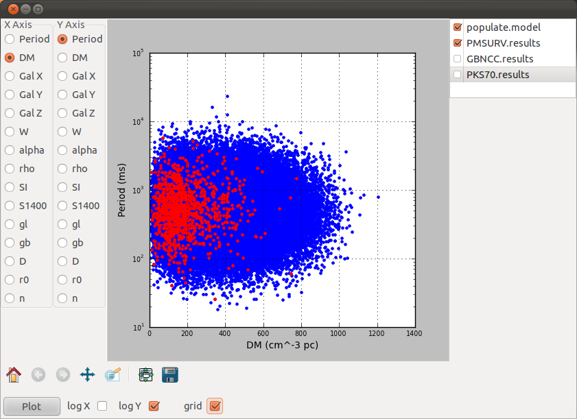
Secondly, PsrPopPy provides an interactive graphical user interface for plotting pulsar parameters against one another (for a screenshot see Figure 1). Users can select models in the current working directory to be plotted, select which parameters to plot, and choose to plot using linear or logarithmic $x$ and $y$ axes. Plots can also be saved in various file formats, including vector formats such as postscript.

4.6 Combining PsrPopPy functions

PsrPopPy has been designed to allow user-generated scripts to be simple to implement. All population models are written in a uniform format and, in fact, are simply serialised objects from the code. This means that no code is required to parse models back into memory, and that high-level scripts can be used to pass a model directly between codes, without having to write to disk and then read it out again. This also removes the need to modify the codebase whenever additional parameters are added to the models, making the code more robust.

5 Applications of PsrPopPy

5.1 Spectral Index Distribution

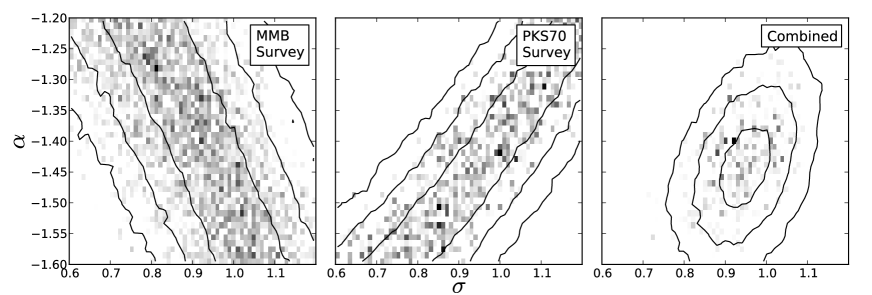
In order to test the ability of PsrPopPy to reproduce results previously obtained with PsrPop, we first ran simulations following Bates et al. (2013, see § 4 of that paper for details of the method), to determine the spectral index distribution of normal pulsars. The only difference allowed was to perform only 50 realisations per bin instead of 500. We are able to reproduce the Figure 1 of Bates et al., shown here in Figure 2, which in turn would lead to the same conclusions reached in that work — the best-fitting spectral index distribution from these simulations is $\alpha=-1.4$, $\beta=1.0$.

5.2 Modelling the pulsar luminosity distribution

As discussed in § 2.3, the pulsar luminosity distribution is sometimes parameterised in terms of the period, $P$, and period derivative, $\dot{P}$, using the formulation show in Equation 6. In this section, we use the evolutionary simulation code evolve to estimate the value of the parameters $\alpha$ and $\beta$ in this equation. We kept value of $\gamma$ in this equation fixed at $0.18\mathrm{~{}mJy~{}kpc}^{2}$, the optimal value according to FK06.

For values of $\alpha$ and $\beta$ covering a grid covering the range $-1.6<\alpha<0.8$ and $0.3<\beta<0.7$, model pulsar populations were generated using evolve as per the specifications outlined in Table 2. The populations were grown until 1206 pulsars per population were detected in simulations of the Parkes multibeam pulsar survey (PMSURV, Manchester et al., 1996) and the two Swinburne pulsar surveys at higher Galactic latitudes (Edwards et al., 2001; Jacoby et al., 2009). This is the number of normal pulsars (defined as $P>30\mathrm{~{}ms}$, $\dot{P}<1\times 10^{-12}$) listed in the pulsar catalogue (Manchester et al., 2005) as detected by any one or more of these three surveys.

For each grid point $(\alpha,\beta)$, 25 realisations of the simulation were performed. For each, the $P$ and $\dot{P}$ values of the resulting population model were compared to those of the 1206 pulsars listed in the pulsar catalogue using the 2-dimensional Kolmogorov-Smirnov test (Press et al., 1986). While the probabilities generated by this algorithm are not statistically rigorous, this test does provide a helpful way of quantifying how well two 2-d distributions match one another. The average value of this probability over the 25 realisations was stored, as were the models generated by dosurvey.

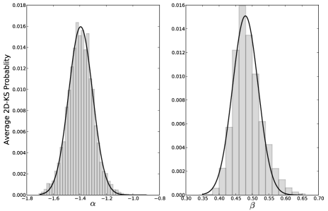
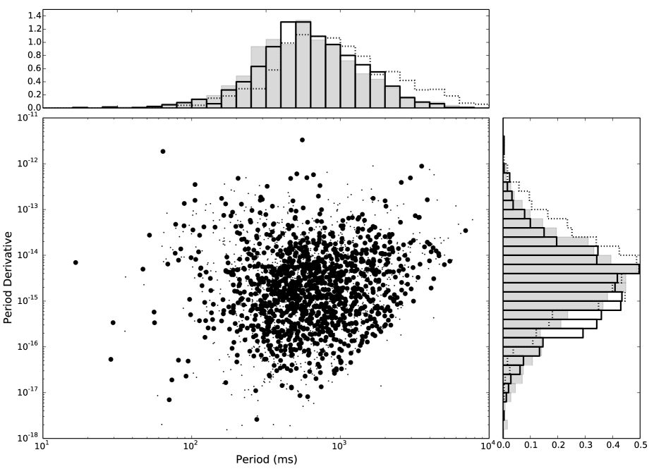
Marginalising over $\alpha$ and then $\beta$ in turn, by averaging the probabilities for each $\alpha$ or $\beta$ value, the distributions shown in Figure 3 were obtained. Fitting Gaussian functions to these probability distributions, we obtained best-fit values of $\bar{\alpha}=-1.39\pm 0.09$ and $\bar{\beta}=0.48\pm 0.04$. An example $P$-$\dot{P}$ diagram generated using these values for $\alpha$ and $\beta$ is then shown in Figure 4. Histograms are also shown for a simulation using the values $\alpha=-1.0,\beta=0.7$, and are clearly skewed to longer periods and higher values of the period derivative.

It is worth noting that while we have derived values of $\alpha$ and $\beta$ by comparing our simulations to the known pulsar population, we have obtained a very similar result to Perera et al. (2013). Their analysis considered the relationship for gamma-ray luminosities, $P$ and $\dot{P}$, and derived values of $\alpha=-1.36\pm 0.03$ and $\beta=0.44\pm 0.02$. This one-to-one correspondence between empirical luminosities is remarkable given that the fraction of the spin-down energy loss going into gamma-ray emission is substantially greater than in the radio. The X-ray emission does not scale in a similar manner for rotation-powered pulsars (e.g. Possenti et al., 2002; Kargaltsev et al., 2012). Further theoretical studies to explain these results are definitely warranted, and we plan to explore this further in future work.

Figure 5: Histograms of pulsar luminosities for each ‘real age’ bin. Fitted Gaussians are shown with a solid black line.

Figure 6: Normalised histograms (grey bars) of pulsar luminosities for each characteristic age bin. Fitted Gaussians are shown with a solid black line. The dotted lines show normalised histograms of the pulsars detected in a model all-sky survey with the SKA.

5.3 Scaling laws for the underlying population

Having, in the previous section, constrained the values of $\alpha$ and $\beta$ in Equation 6, we then should be able to see how pulsar luminosities vary with age (both the ‘real’ age, $\tau_{\mathrm{real}}$ in our simulations, and the characteristic age, given by $\tau_{\mathrm{char}}=P/2\dot{P}$).

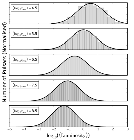
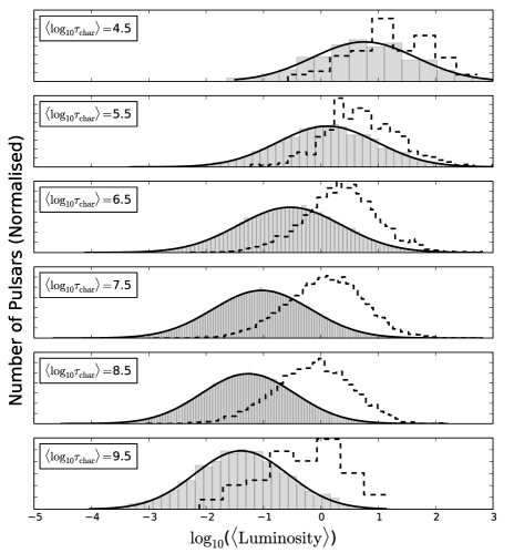
First, a model was created using the best values $\alpha=-1.39$, $\beta=0.48$. Using only pulsars in the population which lie above the deathline (and are, therefore, considered to be emitting radiation), the population was then divided into logarithmic bins in both real and characteristic ages (with centre values $\log_{10}\tau=4.5,5.5...,9.5$ for $\tau$ in years). For each of the age bins, histograms were made of pulsar luminosity (shown in Figures 5 and 6). The histograms were fitted with Gaussians of mean, $\mu$ and standard deviation $\sigma$, and the fitted values of $\mu$ and $\sigma$, with the errors on these values taken from the resultant covariance matrix, are then plotted in Figure 7.

Figure 7: Mean (upper) and standard deviation (lower) values, with associated errors, from the fits performed in Figures 5 (left) and 6 (right). Upper panels are fit by an exponential decay, the lower panels with a linear decay.

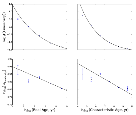
The results from Figure 7 are that we can characterise the change in pulsar luminosity, $L$, with the logarithm of age (both real age and characteristic age) as an exponential decay,

$$\log_{10}L\propto\exp\left(-\frac{\log_{10}\tau}{\log_{10}\tau_{\mathrm{decay}}}\right)+a.$$ (31)

We obtained best fits of $\log\tau_{\mathrm{decay}}=2.6\pm 0.8$, $a=-1.9\pm 0.3$ when considering real ages, and $\log\tau_{\mathrm{decay}}=2.1\pm 0.4$, $a=-1.7\pm 0.2$ for the characteristic ages.

The width of the luminosity distributions is also seen to change, shown in the lower panels of Figure 7. We model this change as

$$\log_{10}\sigma_{L}=b\log_{10}\tau+c.$$ (32)

We obtained best fitting values of $b=-0.031\pm 0.006,c=1.08\pm 0.05$ for pulsar real ages, and $b=-0.034\pm 0.006,c=1.11\pm 0.05$ in the case of characteristic ages.

Our simulations show, however, that the currently-known pulsar population (simulated using a sub-sample detected by PMSURV and the Swinburne pulsar surveys) does not contain enough low-luminosity pulsars to be able to measure this age-luminosity relationship. However, as shown in Figure 6, the large number of pulsars expected to be discovered in all-sky surveys using the SKA (see, e.g., Smits et al., 2009a), may begin to probe this relationship.

6 Conclusions

We have developed a software packge for the simulation of the Galactic pulsar population. The package has been written mainly in Python, with reliance on some older Fortran code for complex calculations. Using this software, we have demonstrated possible applications of the code:

• in § 5.1 we reproduced the results of Bates et al. (2013), who characterised the spectral index distribution of normal pulsars as a Gaussian with mean $-1.4$ and standard deviation $1.0$;

• in § 5.2, the pulsar luminosity distribution was characterised in terms of the pulsar period, $P$, and period derivative, $\dot{P}$. We obtained best-fit values for the power-law indices $\alpha$ and $\beta$ of $\alpha=-1.39\pm 0.09$ and $\beta=0.48\pm 0.04$;

• in § 5.3 we looked at how the pulsar luminosity distribution varies with pulsar ages (both real and characteristic). It was seen that, regardless of whether real or characteristic age is used, $\log_{10}L$ falls exponentially with $\log_{10}\tau$ with a decay constant of 2.1–2.6.

Further functionality will be added to the PsrPopPy code in the future, including:

• an improved treatment of millisecond pulsars, including models of binary parameters;

• using these binary parameters to model the effect of binary motion on signal strength in pulsar surveys (e.g.  Bagchi et al., 2013);

• the inclusion of pulse intensity distributions, and the extension of these to include rotating radio transients (RRATs);

• model the effects of scintillation on low-DM pulsars (e.g.  Cordes & Chernoff, 1997).

Once some of these features have been implemented, it may become possible to repeat the simulations we have performed here, or others similar to them, instead focussing on the millisecond pulsars, or RRATs. It may also be useful to include these pulsars in predictions for future surveys. Of course, as the number of such known sources increases, there will be better statistical models to be included in PsrPopPy, in turn increasing the accuracy of the software.

References

- Bagchi et al. (2013) Bagchi M., Lorimer D. R., Wolfe S., 2013, MNRAS, 432, 1303
- Bates et al. (2011a) Bates S. D. et al., 2011a, MNRAS, 416, 2455
- Bates et al. (2011b) Bates S. D. et al., 2011b, MNRAS, 411, 1575
- Bates et al. (2013) Bates S. D., Lorimer D. R., Verbiest J. P. W., 2013, MNRAS, 431, 1352
- Bhat et al. (2004) Bhat N. D. R., Cordes J. M., Camilo F., Nice D. J., Lorimer D. R., 2004, ApJ, 605, 759
- Bhattacharya et al. (1992) Bhattacharya D., Wijers R. A. M. J., Hartman J. W., Verbunt F., 1992, A&A, 254, 198
- Boyles et al. (2012) Boyles J. et al., 2012, ArXiv e-prints
- Burgay et al. (2006) Burgay M. et al., 2006, MNRAS, 368, 283
- Carlberg & Innanen (1987) Carlberg R. G., Innanen K. A., 1987, AJ, 94, 666
- Contopoulos & Spitkovsky (2006) Contopoulos I., Spitkovsky A., 2006, ApJ, 643, 1139
- Cordes & Chernoff (1997) Cordes J. M., Chernoff D. F., 1997, ApJ, 482, 971
- Cordes & Lazio (2002) Cordes J. M., Lazio T. J. W., 2002, ArXiv Astrophysics e-prints (astro-ph/0207156)
- Edwards et al. (2001) Edwards R. T., Bailes M., van Straten W., Britton M. C., 2001, MNRAS, 326, 358
- Faucher-Giguère & Kaspi (2006) Faucher-Giguère C. A., Kaspi V. M., 2006, ApJ, 643, 332, in press
- Gil et al. (1984) Gil J., Gronkowski P., Rudnicki W., 1984, A&A, 132, 312
- Jacoby et al. (2009) Jacoby B. A., Bailes M., Ord S. M., Edwards R. T., Kulkarni S. R., 2009, ApJ, 699, 2009
- Kargaltsev et al. (2012) Kargaltsev O., Durant M., Pavlov G. G., Garmire G., 2012, ApJS, 201, 37
- Keith et al. (2010) Keith M. J. et al., 2010, MNRAS, 409, 619
- Kramer et al. (1998) Kramer M., Xilouris K. M., Lorimer D., Doroshenko O., Jessner A., Wielebinski R., Wolszczan A., Camilo F., 1998, ApJ, 501, 270
- Kuijken & Gilmore (1989) Kuijken K., Gilmore G., 1989, MNRAS, 239, 651
- Levin et al. (2013) Levin L. et al., 2013, MNRAS, 434, 1387
- Lorimer (2012) Lorimer D. R., 2012, ArXiv e-prints
- Lorimer et al. (1993) Lorimer D. R., Bailes M., Dewey R. J., Harrison P. A., 1993, MNRAS, 263, 403
- Lorimer et al. (2006) Lorimer D. R. et al., 2006, MNRAS, 372, 777
- Lorimer & Kramer (2005) Lorimer D. R., Kramer M., 2005, Handbook of Pulsar Astronomy. Cambridge University Press
- Lorimer et al. (1995) Lorimer D. R., Yates J. A., Lyne A. G., Gould D. M., 1995, MNRAS, 273, 411
- Lyne (1998) Lyne A. G., 1998, Advances in Space Research, 21, 149
- Lyne et al. (1985) Lyne A. G., Manchester R. N., Taylor J. H., 1985, MNRAS, 213, 613
- Manchester et al. (2005) Manchester R. N., Hobbs G. B., Teoh A., Hobbs M., 2005, AJ, 129, 1993
- Manchester et al. (2001) Manchester R. N. et al., 2001, MNRAS, 328, 17
- Manchester et al. (1996) Manchester R. N. et al., 1996, MNRAS, 279, 1235
- Maron et al. (2000) Maron O., Kijak J., Kramer M., Wielebinski R., 2000, A&A, 147, 195
- Narayan (1987) Narayan R., 1987, ApJ, 319, 162
- Perera et al. (2013) Perera B. B. P., McLaughlin M. A., Cordes J. M., Kerr M., Burnett T. H., Harding A. K., 2013, ApJ, 776, 61
- Possenti et al. (2002) Possenti A., Cerutti R., Colpi M., Mereghetti S., 2002, A&A, 387, 993
- Press et al. (1986) Press W. H., Flannery B. P., Teukolsky S. A., Vetterling W. T., 1986, Numerical Recipes: The Art of Scientific Computing. Cambridge University Press, Cambridge
- Ridley & Lorimer (2010) Ridley J. P., Lorimer D. R., 2010, MNRAS, 404, 1081
- Schnitzeler (2012) Schnitzeler D. H. F. M., 2012, MNRAS, 427, 664
- Smits et al. (2009a) Smits R., Kramer M., Stappers B., Lorimer D. R., Cordes J., Faulkner A., 2009a, A&A, 493, 1161
- Smits et al. (2009b) Smits R., Lorimer D. R., Kramer M., Manchester R., Stappers B., Jin C. J., Nan R. D., Li D., 2009b, A&A, 505, 919
- Taylor & Manchester (1977) Taylor J. H., Manchester R. N., 1977, ApJ, 215, 885
- Weltevrede & Johnston (2008) Weltevrede P., Johnston S., 2008, MNRAS, 387, 1755
- Yusifov & Küçük (2004) Yusifov I., Küçük I., 2004, A&A, 422, 545