Strong dynamical effects during stick-slip adhesive peeling

Marie-Julie Dalbe, Stéphane Santucci, Pierre-Philippe Cortet, and Loïc Vanel

(Dated: November 14, 2013)

We consider the classical problem of the stick-slip dynamics observed when peeling a roller adhesive tape at a constant velocity. From fast imaging recordings, we extract the dependencies of the stick and slip phases durations with the imposed peeling velocity and peeled ribbon length. Predictions of Maugis and Barquins [in Adhesion 12, edited by K.W. Allen, Elsevier ASP, London, 1988, pp. 205–222] based on a quasistatic assumption succeed to describe quantitatively our measurements of the stick phase duration. Such model however fails to predict the full stick-slip cycle duration, revealing strong dynamical effects during the slip phase.

1 Introduction

Everyday examples of adhesive peeling are found in applications such as labels, stamps, tape rollers, self-adhesive envelops or post-it notes. During the peeling of those adhesives, a dynamic instability of the fracture process corresponding to a jerky advance of the peeling front and called “stick-slip” may occur. This stick-slip instability has been an industrial concern since the 1950’s because it leads to noise levels above the limits set by work regulations, to adhesive layer damage and/or to mechanical problems on assembly lines. Nowadays this instability is still a limiting factor for industrial productivity due to the limitations of generic technical solutions applied to suppress it, such as anti-adhesive silicon coating.

From a fundamental point of view, the stick-slip instability of adhesive peeling is generally understood as the consequence of an anomalous decrease of the fracture energy $\Gamma(v_{p})$ of the adhesive-substrate joint in a specific range of peeling front velocity $v_{p}$. ^{1, 2, 3, 5, 6, 7, 8, 4} Indeed, when the peeling process also involves a compliance between the point where the peeling velocity is imposed and the fracture front, this decreasing fracture energy naturally leads to oscillations of the fracture velocity $v_{p}$ around the mean velocity $V$ imposed by the operator. Often, it is simply the peeled ribbon elasticity which provides a compliance to the system. From a microscopic perspective, such anomalous decrease of the fracture energy $\Gamma(v_{p})$ (correctly defined for stable peeling only) could correspond (but not necessarily) to transition from cohesive to adhesive failure ^{2, 3} or between two different interfacial failure modes. ^{7, 4} More fundamentally, this decrease of the fracture energy has been proposed to be the consequence of the viscous dissipation in the adhesive material. ⁹ De Gennes ¹⁰ further pointed out the probable fundamental role of the adhesive material confinement (which was evidenced experimentally in ref. 3) in such viscoelastic theory. Since then, it has however appeared that a model based on linear viscoelasticity solely cannot be satisfactory and that the role of creep, large deformations and temperature gradient in the adhesive material is important (refs. 11, 12, 13, 14 and references therein).

Experimentally, the stick-slip instability was first characterized thanks to peeling force measurements which revealed strong fluctuations in certain ranges of peeling velocity. ^{1, 3, 5, 6} Since then, it has also been studied through indirect measurements of the periodic marks left on the tape ^{15, 5, 16, 6} or of the emitted acoustic noise. ^{17, 18} Thanks to the progress in high speed imaging, it is now possible to directly access the peeling fracture dynamics in the stick-slip regime. ^{19, 20, 21}

In the late 1980’s, Barquins and co-workers, ^{5, 6} performed a series of peeling experiments of a commercial adhesive tape (3M Scotch^® 602) at constant pulling velocity $V$ and for various lengths of peeled ribbon $L$. For the considered adhesive, the velocity range for which stick-slip was evidenced, thanks to peeling force fluctuations measurements, was shown to be $0.06<V<2.1$ m s^-1. In a subrange of unstable peeling velocity $0.06<V<0.65$ m s^-1, the authors succeeded to access the stick-slip cycle duration thanks to the post-mortem detection of periodic marks left on the tape by stick-slip events. Moreover, they managed to model quantitatively the measured stick-slip period, ^{5, 6} assuming the fracture dynamics to remain a quasistatic problem during the stick phase and backing on measurements of the stable branch of the fracture energy $\Gamma(v_{p})$ at low peeling velocities below the instability onset.

In this article, we revisit these experiments by studying the stick-slip dynamics during the peeling of a roller adhesive tape at an imposed velocity. The principal improvement compared to Barquins’s seminal work is that, thanks to a high speed camera coupled to image processing, we are able to access the dynamics of the peeling fracture front. We focus on the study of the duration of the stick-slip cycle and its decomposition into stick and slip events, which data are inaccessible through other techniques. We present experimental data of the stick and slip durations for a wide range of imposed peeling velocity $V$ and for different peeled ribbon lengths $L$. We show that the model proposed by Barquins and co-workers ^{5, 6} describes the evolution of the duration of the stick phase, but fails to predict the duration of the whole stick-slip cycle due to unexpectedly long slip durations.

2 Experimental setup

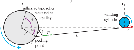
Figure 1: (Color online) Schematic view of the experimental setup. The angles $\alpha$ and $\beta$ are oriented clockwise and counterclockwise respectively. Roller diameter: $40$ mm $<2R<58$ mm, roller and tape width: $b=19$ mm.

In this section, we describe briefly the experimental setup which has already been presented in details in a recent work. ²¹ We peel an adhesive tape roller (3M Scotch^® $600$, made of a polyolefin blend backing coated with a layer of a synthetic acrylic adhesive, also studied in refs. 19, 21, 8), mounted on a freely rotating pulley, by winding up the peeled ribbon extremity on a cylinder at a constant velocity $V$ using a servo-controlled brushless motor (see Fig. 1). The experiments have been performed at a temperature of $23\pm 2^{\mathrm{o}}$ and a relative humidity of $45\pm 5$%. The width of the tape is $b=19$ mm, its thickness $e=38~{}\mu$m and its Young modulus $E=1.26$ GPa.

Each experiment consists in increasing the winding velocity from $0$ up to the target velocity $V$. Once the velocity $V$ is reached, it is maintained constant during two seconds before decelerating the velocity back to zero. When stick-slip is present this 2-second stationary regime of peeling provides sufficient statistics to compute well converged stick-slip mean features. We have varied the imposed velocity $V$ from $0.0015$ to $2.5$ m s^-1 for different values of the peeled tape length between $L=0.08$ and $1.31$ m. During an experiment, the peeled tape length $L$ (Fig. 1) is submitted to variations, due to the stick-slip fluctuations and to slow oscillations of the peeling point angular position, which however always remain negligible compared to its mean value (less than 0.3%). ²¹

3 Peeling force measurement

Thanks to a force sensor (Interface^® SML-5) on the holder maintaining the pulley, we are able to measure the mean value of the force $F$ transmitted along the peeled tape during one experiment. When peeling is stable, we compute the strain energy release rate $G$ from the mean value of the force $F$, following the traditional relation for the peeling geometry ^{22, 23}

$$G=\frac{F}{b}(1-\cos\theta)+\frac{1}{2Ee}\left(\frac{F}{b}\right)^{2}\simeq\frac{F}{b},$$ (1)

for a peeling angle $\theta\simeq 90^{\mathrm{o}}$ (see Fig. 1). The quantity $G$ corresponds to the amount of mechanical energy released by the growth of the fracture by a unit surface. The right-hand term of eqn (1) finally simply takes into account the work done by the operator but discards the changes in the elastic energy stored in material strains (term $(F/b)^{2}/2Ee$ in eqn (1)) ²³ which are negligible here. Indeed, the maximum encountered force in our experiments is typically of about $2$ N, which gives $F/b\approx 100$ J m^-2, to be compared to $(F/b)^{2}/2Ee\approx 0.12$ J m^-2.

In the context of elastic fracture mechanics, the condition for a fracture advance at a constant velocity $v_{p}$ is a balance between the release rate $G$ and a fracture energy $\Gamma(v_{p})$ required to peel a unit surface and accounting for the energy dissipation near the fracture front. When the fracture velocity $v_{p}$ approaches the Rayleigh wave velocity $v_{R}$, $\Gamma(v_{p})$ also takes into account the kinetic energy stored in material motions which leads to a divergence when $v_{p}\rightarrow v_{R}$. ²⁴ In our system, the strain energy release rate $G$, computed through eqn (1), therefore stands as a measure of the fracture energy $\Gamma(v_{p})$ when the peeling is stable only, i.e. when $v_{p}$ is constant. We will nevertheless compute $G$ for the experiments in the stick-slip regime for which the peeling fracture velocity $v_{p}(t)$ is strongly fluctuating in time. In such a case, $G$ cannot be used as a measure of a fracture energy: it is simply the time average of the peeling force $F$ in units of $G$.

In Fig. 2, we plot $G$ as a function of the imposed peeling velocity $V$ for three different peeled tape lengths $L$. When the peeling is stable, the peeling force is nearly constant in time, whereas it fluctuates strongly when stick-slip instability is present. The standard deviation of these fluctuations is represented in Fig. 2 with error bars. Large error bars are indicative of the presence of stick-slip.

Between $V=0.0015$ m s^-1 and $V=0.10\pm 0.03$ m s^-1, we observe that $G=F/b$ increases slowly with $V$ and that its temporal fluctuations are nearly zero, revealing that the peeling is stable. This increasing branch $G(V)$ is therefore a measure of the adhesive fracture energy $\Gamma(v_{p}=V)=G(V)$ for $V<0.10\pm 0.03$ m s^-1. Our results are compatible with the data reported by Barquins and Ciccotti ⁸ for the same adhesive tape (see Fig. 2). However, they explored a much larger range of velocities in this stable branch of peeling, down to $V=10^{-5}$ m s^-1. Using both series of measurements, it is reasonable to model the stable peeling branch with a power law, $G(V)=a\,V^{n}$, with $n=0.146$ and $a=137$. For $0.10\pm 0.03$ m s${}^{-1}<V\leqslant 2.5$ m s^-1, we observe that the measured value of $G(V)$ decreases with $V$. This tendency, which was already observed in previous experiments, ²⁵ is accompanied with the appearance of temporal fluctuations which are the trace of the stick-slip instability. From these data, we can estimate the onset of the instability to be $V_{a}=0.10\pm 0.03$ m s^-1. The measured decreasing branch of $G(V)$ for $V>V_{a}$ appears as a direct consequence of the anomalous decrease of the fracture energy at the origin of the instability. It is important to note that the measured mean value of $G=F/b$ is nearly independent of the length of peeled ribbon $L$. This result is natural in the stable peeling regime but was a priori unknown in the stick-slip regime.

Barquins and Ciccotti ⁸ succeeded to measure a second stable peeling branch for $V\geqslant 19$ m s^-1. This increasing branch constitutes a measure of the peeling fracture energy $\Gamma(v_{p}=V)=G(V)$ in a fast and stable peeling regime. In ref. 8, this branch is inferred to exist for velocities even lower than $V=19$ m s^-1, although it was not possible to measure it. Backing on the data of ref. 6 for a very close adhesive, one can however guess that the local minimum value of $G(V)$, corresponding to a velocity in the range $2.5$ m s${}^{-1}<V<19$ m s^-1, would be bounded by $G_{0,1}=18<G<G_{0,2}=33$ J m^-2.

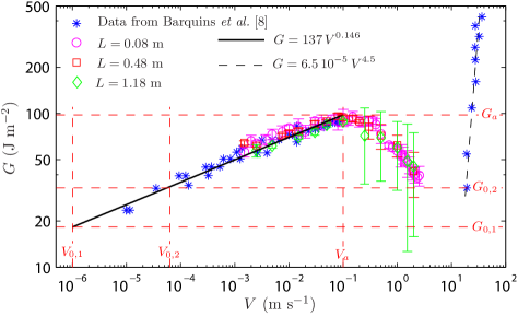
Figure 2: (Color online) Mean value of the peeling force $F$, in units of strain energy release rate $G=F/b$, as a function of $V$ for 3 different peeled tape lengths $L$. Stars report the data of Barquins and Ciccotti ⁸ for the same adhesive. Solid line is a power law fit $G=137\,V^{0.146}$ of the data in the low velocity stable branch. Errorbars represent the standard deviation of the force fluctuations during one experiment.

4 Peeling point dynamics

The local dynamics of the peeling point is imaged using a high speed camera (Photron FASTCAM SA4) at a rate of $20\,000$ fps. The recording of each movie is triggered once the peeling has reached a constant average velocity $V$ ensuring that only the stationary regime of the stick-slip is studied. Through direct image analysis, ²¹ the movies allow access to the curvilinear position of the peeling point $\ell_{\alpha}(t)=R\,\alpha$ in the laboratory frame (with $\alpha$ the angular position of the peeling point and $R$ the roller diameter, $\alpha>0$ in Fig. 1). Image correlations on the adhesive tape roller contrast pattern further allow direct access to its angular velocity $d\beta/dt(t)$ in the laboratory frame (where $\beta$ is the unwrapped angular position of the roller, $\beta>0$ in Fig. 1, $\ell_{\beta}(t)=R\,\beta$). We finally compute numerically the curvilinear position $\ell_{p}(t)=\ell_{\beta}(t)+\ell_{\alpha}(t)$ and velocity $v_{p}(t)=d\ell_{p}/dt$ of the peeling point in the roller reference frame.

The curvilinear position of the peeling point $\ell_{\alpha}(t)$ in the laboratory frame is actually estimated from the position of the peeled ribbon at a small distance $0.30\pm 0.05$ mm from the peeling fracture front on the roller surface. We therefore do not detect strictly the peeling fracture front position but a very close quantity only. This procedure can consequently introduce some bias in our final estimation of the fracture front velocity $v_{p}(t)$. This bias is notably caused by the changes in the radius of curvature of the tape at the junction with the substrate which are due to the force oscillations in the peeled tape characteristics of the stick-slip instability. Such effect actually biases the measurement toward larger velocities during the stick phase and lower velocities during the slip phase. Another effect that leads to uncertainties on velocity measurement is the emission of a transverse wave in the peeled tape when the fracture velocity abruptly changes at the beginning and at the end of slip phases.

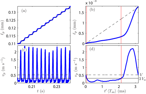
Figure 3: (Color online) (a) Peeling point position $\ell_{p}(t)$ in the roller reference frame for an experiment performed at $V=0.55$ m s^-1 and $L=0.47$ m. The dashed line shows $\ell_{p}=V\,t$, with $V$ the average peeling velocity. (b) Corresponding phase averaged peeling point position as a function of $t^{\prime}\,\langle T_{ss}\rangle$ (see main text). (c) and (d) Corresponding instantaneous (c) and phase averaged (d) peeling point velocity $v_{p}$. The dashed horizontal lines show the average peeling velocity $V$ and the continuous horizontal lines show $3\,V_{a}$. In (b) and (d), the vertical lines show the transitions between the stick ($v_{p}<3\,V_{a}$) and the slip ($v_{p}>3\,V_{a}$) phases.

Figs. 3(a) and (c) represent the fracture position $\ell_{p}(t)$ and velocity $v_{p}(t)$ as a function of time for a typical experiment performed at $V=0.55$ m s^-1 and $L=0.47$ m. In these figures, we observe alternate phases of slow –stick phase– and fast –slip phase– peeling which are the signature of the stick-slip motion. These large velocity fluctuations are quite regular in terms of duration and to a lesser extent in terms of amplitude at least at the considered peeling velocity. Our general data analysis further consists in the decomposition of the signal of instantaneous peeling velocity $v_{p}(t)$ into stick-slip cycles by setting the beginning of each cycle at times $t_{n}$ ($n$ denoting the $n^{th}$ cycle) when $v_{p}(t_{n})=V$ and $dv_{p}/dt(t_{n})<0$. From this data, we extract the duration $T_{ss}$ of each stick-slip cycle for which we define a rescaled time $t^{\prime}=(t-t_{n})/T_{ss}$. We further compute the phase averaged evolution of the peeling fracture velocity $v_{p}(t^{\prime})$ from $t^{\prime}=0$ to $1$ considering all the stick-slip cycles in one experiment. With this procedure, we finally extract for each peeling velocity $V$ and peeled tape length $L$ the typical fracture velocity evolution during a stick-slip cycle getting rid of intrinsic fluctuations of the stick-slip period. In Figs. 3(b) and (d), we show the phase averaged position and velocity profiles, corresponding to Figs. 3(a) and (c) respectively, as a function of $t=t^{\prime}\,\langle T_{ss}\rangle$ ($\langle\,\rangle$ denotes the ensemble averaged value over all the cycles in one experiment).

From these phase averaged velocity profiles, we define, for each experimental condition $V$ and $L$, stick events as continuous periods during which $v_{p}(t)<3\,V_{a}$ and slip events as continuous periods during which $v_{p}(t)>3\,V_{a}$. According to the model of Barquins et al. ^{5, 6} a natural threshold in order to separate the stick and slip phases is the onset of the instability $V_{a}$ (as defined in Fig. 2). However, as discussed previously, due to the procedure used for the detection of the peeling point, our measurement of the fracture velocity can be affected by biases caused by the variation the tape curvature at the peeling point and by the propagation of transverse waves in the tape. The effect of the later can be observed in Fig. 3(d) in the early stage of the stick phase. In order to avoid taking into account the velocity biases in the decomposition of the stick-slip cycle, we chose for the threshold separating the stick and slip phases a value little larger the “theoretical” threshold $V_{a}$, that is to say $3\,V_{a}$.

Finally, as we have shown recently in ref. 21, when the peeling velocity $V$ is increased, low frequency pendular oscillations of the peeling angle $\theta$ develop. Due to a dependence of the stick-slip instability onset with the mean peeling angle, these oscillations lead to intermittencies in the stick-slip dynamics for peeling velocities $V>1.5$ m s^-1. We therefore exclude the experiments with $V>1.5$ m s^-1 in the sequel. For the studied experiments, we have a mean peeling angle $\langle\theta\rangle=90\pm 3^{\mathrm{o}}$ with slow temporal variations in the range $\Delta\theta=\pm 15^{\mathrm{o}}$ during one experiment.

5 Stick-slip cycle duration

From the signal of peeling point position $\ell_{p}(t)$ (see Fig. 3(a)), we define the stick-slip amplitude $A_{ss}$ as the distance travelled by the fracture during a stick-slip cycle. In Fig. 4, we report this amplitude $A_{ss}$ for each stick-slip event as a function of the corresponding stick-slip period $T_{ss}$, for all events in 6 different experiments. These data gather close to the curve $A_{ss}=V\,T_{ss}$. The large spread of the data along the curve $A_{ss}=V\,T_{ss}$ reflects the statistics of the stick-slip cycle amplitude and duration which could be due for instance to adhesive heterogeneities. On the contrary, the dispersion of the data around the curve $A_{ss}=V\,T_{ss}$ is much smaller. It actually estimates the discrepancy between the imposed velocity $V$ and the averaged fracture velocity for each stick-slip cycle. The observed small discrepancy actually both traces back measurement errors on the instantaneous fracture velocity and intrinsic fluctuations of the dynamics.

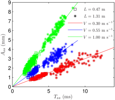
Figure 4: (Color online) Stick-slip amplitude $A_{ss}$ as a function of stick-slip period $T_{ss}$ for each stick-slip cycle in 6 different experiments with $L=0.47$ and $1.31$ m and $V=0.30$, $0.55$ and $1.00$ m s^-1. The lines represent the curves $A_{ss}=V\,T_{ss}$.

In Fig. 4, one can already see that the statistically averaged values of $A_{ss}$ and $T_{ss}$ increase with $L$ for a given peeling velocity $V$. In the following, we will focus on the study of the statistical average $\langle T_{ss}\rangle$ of the duration of the stick-slip oscillation and its decomposition into stick and slip phases with in mind the aim of testing the description of Barquins, Maugis and co-workers. ^{5, 6} There is no need to study the averaged stick-slip amplitude $\langle A_{ss}\rangle$ since it is univocally related to $\langle T_{ss}\rangle$ through $\langle A_{ss}\rangle=V\,\langle T_{ss}\rangle$.

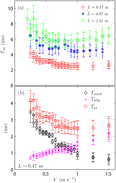
Figure 5: (Color online) Average stick-slip cycle duration $T_{ss}$ as a function of the average peeling velocity $V$, for different lengths of the peeled ribbon $L$. (b) Average stick-slip, stick and slip durations as function of the average peeling velocity for $L=0.47$ m. Each data point corresponds to the average and each error bar to the standard deviation of the statistics over one experiment.

In Fig. 5(a), we plot the mean stick-slip duration $T_{ss}$ as a function of $V$ for three different lengths $L$ of the peeled ribbon. The data corresponds to the average $\langle T_{ss}\rangle$ and the error bars to the standard deviation of the statistics of $T_{ss}$ over all the stick-slip events in each experiment. In the following, since we will consider the averaged values only, we will skip the brackets $\langle\,\rangle$. At first sight, it appears that, within the error bars, the stick-slip duration $T_{ss}$ is stable over the major part of the explored range of peeling velocity $V$. One can however note that, independently of $L$, $T_{ss}$ tends to decrease with $V$ for $V\leqslant V_{c}=0.6\pm 0.1$ m s^-1. Such behavior is compatible with the observations of Barquins et al. ⁵ but appears here over a rather limited velocity range. The characteristic velocity $V_{c}=0.6\pm 0.1$ m s^-1 above which $T_{ss}$ is nearly constant seems not to depend strongly on the length of the peeled ribbon $L$.

In Fig. 5(b), we show the mean durations of stick and slip events, $T_{stick}$ and $T_{slip}$ respectively, as a function of the imposed peeling velocity $V$ for the experiments performed with the peeled length $L=0.47$ m. Interestingly, we observe that the stick and slip phases evolve differently with $V$: the stick duration decreases with $V$, while the slip duration increases over the whole explored range of $V$. In consequence, the ratio $T_{stick}/T_{slip}$, presented in Fig. 6, decreases with $V$ from $T_{stick}/T_{slip}\sim 4\pm 1$ down to $T_{stick}/T_{slip}\sim 0.3\pm 0.2$. Such behavior of $T_{stick}/T_{slip}$ appears to be very little dependent on $L$ according to Fig. 6. For $V\geqslant 0.90\pm 0.05$ m s^-1, $T_{stick}/T_{slip}$ becomes smaller than 1, meaning that the slip phase is longer than the stick one. Our data therefore show that it is not possible to neglect the slip duration compared to the stick duration in general.

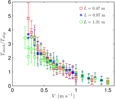
Figure 6: (Color online) $T_{stick}/T_{slip}$ vs. $V$ for 3 different $L$. Each data point corresponds to the average and each error bar to the standard deviation of the statistics over one experiment.

6 Model

In this section, we compare our experimental data with the model proposed by Barquins, Maugis and co-workers in refs. 5, 6. This model is based on measurements of the stable branch of the fracture energy $\Gamma(v_{p})$ for low peeling velocities below the instability onset $V_{a}$, and on the following assumptions:

• During the stick phase, the equilibrium between the instantaneous energy release rate $G=F/b$ and the fracture energy $\Gamma(v_{p})$ (of the low velocity stable branch) is still valid dynamically, i.e. $G(t)=\Gamma(v_{p}(t))$.

• The peeled ribbon remains fully stretched during the peeling, which means

  $$G=\frac{F}{b}=\frac{Ee}{L}\,u,$$ (2)

  where $u$ is the elongation of the tape of Young modulus $E$ and thickness $e$.

• The slip duration is negligible compared to the stick duration.

Backing on these hypothesis, it is possible to derive a prediction for the stick-slip duration $T_{ss}$. Introducing the inverted function $v_{p}=\Gamma^{-1}(G)$ and noting that $du/dt=V-v_{p}$ (see next paragraph and ref. 21), eqn (2) leads to the dynamical relation

$$\frac{dG}{dt}=\frac{Ee}{L}\,(V-\Gamma^{-1}(G)),$$ (3)

which can be integrated over the stick phase to get

$$T_{stick}=\frac{L}{Ee}\int_{G_{0}}^{G_{a}}\frac{dG}{V-\Gamma_{\rm slow}^{-1}(G)}.$$ (4)

$G_{a}$ is the maximum value of $\Gamma(v_{p})$ at the end of the “slow” stable branch $\Gamma_{\rm slow}(v_{p})$. $G_{0}$ is the minimum value of $\Gamma(v_{p})$ at the beginning of the “fast” stable branch $\Gamma_{\rm fast}(v_{p})$ (see Fig. 2) and is assumed to be also the value of $G$ at which the stick phase starts on the slow branch after a slip phase.

In this model, the ribbon is assumed to remain taut during the whole stick-slip cycle. In order to challenge the validity of this hypothesis, let us estimate the evolution of the elongation $u(t)$ of the tape as a function of time. If we note $P(t)$ the peeling point position and $M$ the point where the peeled tape is winded, we can define the quantity $u(t)$ as the difference between the distance $|\overline{MP(t)}|$ and the length of the peeled tape in the unstrained state. If $u(t)$ is positive, this quantity indeed measures the elongation of the tape as in eqn (2), whereas it measures the excess of slack tape if it is negative. Following ref. 21, one can show that

$$u(t)=u_{0}+\int_{0}^{t}(V-v_{p}(t))dt-\cos\theta\int_{0}^{t}(R\dot{\beta}-v_{p}(t))dt.$$ (5)

Since in our experiments the peeling angle $\theta$ is close to $90^{\mathrm{o}}$ and the roller rotation velocity $R\,d\beta/dt$ sticks to the imposed peeling velocity $V$ to a precision always better than $\pm 1.5\%$, ²¹ we finally have $u(t)\simeq u_{0}+\int_{0}^{t}(V-v_{p}(t))dt$. The elongation/slack $u(t)$ increases of $\Delta u=\int_{0}^{T_{stick}}(V-v_{p}(t))dt$ during the stick phase and decreases of the same amplitude $\Delta u=-\int_{T_{stick}}^{T_{ss}}(V-v_{p}(t))dt$ during the slip phase. This compensation is ensured by the fact the averaged velocity over the stick-slip cycle matches the imposed velocity $V$, i.e. $\int_{0}^{T_{ss}}(V-v_{p}(t))dt=0$, and is valid whether or not the tape remains always taut during the stick-slip cycle.

To test the relevance of the hypothesis of a tape always in tension, one can actually compare the increase/decrease $\Delta u$ of the quantity $u(t)$ during the stick/slip phase to the one predicted by the quasistatic model of Barquins and co-workers

$$\Delta u_{\rm theo}=\frac{L}{Eeb}(F_{a}-F_{0})=\frac{L}{Ee}(G_{a}-G_{0}),$$ (6)

for an always taut tape. Throughout our data, the relative discrepancy $(\Delta u_{\rm theo}-\Delta u)/\Delta u$ is typically less than 15% which confirms the relevance of the assumption of a tape in tension during the whole stick-slip cycle.

An equivalent but more instructive way to test the model of Barquins and co-workers is to integrate numerically eqn (4) and compare it to experimental measurements of stick duration. To do so, we use the fit of the data of energy release rate $G(V)$ of Fig. 2, i.e. $G(V)=\Gamma_{\rm slow}(V)=a\,V^{n}$, with $n=0.146$ and $a=137$. The value of $G_{0}$ is affected by a significant uncertainty in our data. We will therefore use two different guesses corresponding to the limit values introduced at page 3 (see $G_{0,1}$ and $G_{0,2}$ in Fig. 2). These values of $G_{0}$ correspond to two limit values of the fracture velocity at the beginning of the stick phase: $V_{0,1}=10^{-6}$ m s^-1 measured in another adhesive but with a close behavior, ⁶ and $V_{0,2}=6.3\times 10^{-5}$ m s^-1 which is an upper limit for $V_{0}$ according to the data of Fig. 2.

In the insert of Fig. 7(b), we report the measured data for $T_{ss}/L$ as a function of $V$ for three different lengths $L$ as well as the predictions of eqn (4) with $V_{0,1}$ (solid line) and $V_{0,2}$ (dashed line). The model appears compatible with the experimental data only for a marginal range of very low peeling velocities. Once $V>0.5$ m s^-1, the measured values of $T_{ss}/L$ indeed deviates more and more from the theoretical prediction. A first natural explanation for this discrepancy is that the assumption of a negligible slip duration $T_{slip}$ (barely verified for low velocities for which $0.25<T_{slip}/T_{stick}<0.5$) becomes more and more false as $V$ is increased (see Fig. 6).

In Fig. 7(b) we therefore directly plot $T_{stick}/L$ as a function of $V$, along with the prediction (4). One can note that the theoretical predictions using the two limit guesses for $V_{0}$ are not very different. A first interesting result is that the stick duration appears, to the first order, proportional to the peeled tape length $L$ as evidenced by the reasonable collapse of the data $T_{stick}/L$ on a master curve, which is compatible with the analytical prediction of the model (4). But more importantly, we observe that for the range of velocity explored, the model for $T_{stick}$, which do not use any adjustable parameter, reproduces very well the experimental data.

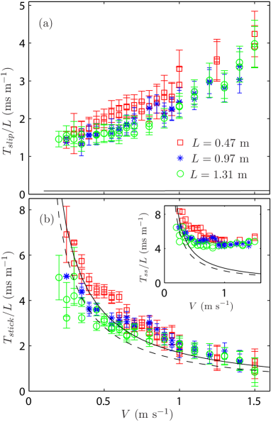
Figure 7: (Color online) (a) $T_{slip}/L$, (b) $T_{stick}/L$ and $T_{ss}/L$ (insert) vs. $V$ for 3 different $L$. Each data point corresponds to the average and each errorbar to the standard deviation of the statistics over one experiment. In (a), the curve close to the $x$-axis represents the theoretical prediction for a quasistationnary slip phase. In (b), the lines show the predictions of eqn (4) with $V_{a}=0.10$ m s^-1 and $V_{0,1}=10^{-6}$ m s^-1 (solid line) or $V_{0,2}=6.3\times 10^{-5}$ m s^-1 (dashed line).

Obviously, one can consider an equivalent quasistationary approximation during the slip phase in order to predict the slip duration using $\Gamma_{\rm fast}^{-1}(G)$ instead of $\Gamma_{\rm slow}^{-1}(G)$ in eqn (4). Here, $\Gamma_{\rm fast}^{-1}(G)$ corresponds to the inverse of the energy fracture $G=\Gamma_{\rm fast}(v_{p})$ in the fast and “stable” peeling regime of Fig. 2. The integration using the model of the fast branch $\Gamma_{\rm fast}(V)=6.5\times 10^{-5}\,V^{4.5}$ (see Fig. 2) however leads to values of $T_{slip}$ always 2 orders of magnitude smaller than the experimental values as evidenced in Fig. 7(a). It is however worth noting that the collapse of the data $T_{slip}/L$ for the different $L$ shows that $T_{slip}$ increases nearly linearly with $L$.

7 Discussion

In this paper, we report experiments of a roller adhesive tape peeled at a constant velocity focusing on the regime of stick-slip instability. From fast imaging recordings, we extract the dependencies of the stick and slip phases durations with the imposed peeling velocity $V$ and peeled ribbon length $L$.

The stick phase duration $T_{stick}$ of the stick-slip oscillations is shown to be nearly proportional to the peeled tape length $L$ and to decrease with the peeling velocity $V$. These data moreover appear in quantitative agreement with the predictions of a model proposed by Barquins, Maugis and co-workers in refs. 5, 6 which do not introduce any adjustable parameter. This successful comparison confirms the relevance of the two main assumptions made in the model: (i) the tape remains in tension during the whole stick-slip cycle; (ii) the principle of an equilibrium between the instantaneous energy release rate $G(t)=F(t)/b$ and the fracture energy $\Gamma(v_{p}(t))$, as measured in the steady peeling regime, is valid dynamically during the stick phase.

Describing the peeling dynamics as a function of time $t$ by the knowledge of the fracture velocity $v_{p}(t)$ and of the force $F(t)=b\,G(t)$ in the peeled tape, the considered model further assumes that the system jumps instantaneously, at the end of the stick phase, from the “slow” stable branch to the “fast” stable branch of the steady fracture energy $G=\Gamma(v_{p})$ and then instantaneously backward from the “fast” branch to the “slow” branch at the end of the slip phase. In such a framework, reproducing the assumptions (i) and (ii) for the slip phase leads to a prediction for the slip duration. We have shown that this prediction is at least hundred times smaller than the slip phase duration $T_{slip}$ measured in our experiments. We actually report that, contrary to what is finally proposed in refs. 5, 6, the slip duration $T_{slip}$ cannot be neglected compared to the stick one $T_{stick}$, since it is at best 4 times smaller, and becomes even larger than $T_{stick}$ for $V\geqslant 0.90\pm 0.05$ m s^-1.

These last experimental results account for the existence of strong dynamical effects during the slip phase which can therefore not be described by a quasistatic hypothesis. These dynamical effects could be due to the inertia of the ribbon close to the fracture front. Some models also predict a strong influence of the roller inertia.^{18, 26} Notably, thanks to numerical computation, De and Ananthakrishna²⁶ have shown that for certain values of the roller inertia, the slip phase could consist in several jumps from the “fast stable” branch to the “slow stable” branch in the $(v_{p},G=\Gamma(v_{p}))$ diagram. Such a process would certainly produce a longer slip time than expected in the framework of Barquins’s model. It would be most interesting to confront our experimental observations to the predictions of this model, based on a detailed set of dynamical equations and ad-hoc assumptions made on the velocity dependence of $\Gamma$. However, such a comparison is not straightforward in our current setup since we do not have the temporal and spatial resolutions to detect such eventual fast oscillations. Besides, in order to obtain a quantitative comparison, measurement of the instantaneous peeling force $F(t)$ is required but it remains a challenge.

References

- 1 J.L. Gardon, J. Appl. Polym. Sci., 1963, 7, 625–641.
- 2 A.N. Gent and R.P. Petrich, Proc. R. Soc. London, Ser. A, 1969, 310, 433–448.
- 3 D.W. Aubrey, G.N. Welding and T. Wong, J. Appl. Polym. Sci., 1969, 13, 2193–2207.
- 4 D.W. Aubrey and M. Sherriff, J. Polym. Sci.,1980, 18, 2597–2606.
- 5 M. Barquins, B. Khandani and D. Maugis, C. R. Acad. Sci. serie II,1986, 303, 1517–1519.
- 6 D. Maugis and M. Barquins, Adhesion 12, edited by K. W. Allen, Elsevier ASP, London, 1988, pp. 205–222.
- 7 C. Derail, A. Allal, G. Marin and P. Tordjeman, J. Adhesion, 1997, 61, 123–157; 1998, 68, 203–228.
- 8 M. Barquins and M. Ciccotti, Int. J. Adhes. Adhes., 1997, 17, 65–68.
- 9 D. Maugis, J. Mater. Sci., 1985 20, 3041–3073.
- 10 P.-G. de Gennes, Langmuir,1996, 12, 4497–4500.
- 11 A.N. Gent, Langmuir, 1996, 12, 4492–4496.
- 12 G. Carbone and B.N.J. Persson, Phys. Rev. Lett., 2005, 95, 114301.
- 13 E. Barthel and C. Fretigny, J. Phys. D Appl. Phys., 2009, 42, 19.
- 14 H. Tabuteau, S. Mora, M. Ciccotti, C.-Y. Hui and C. Ligoure, Soft Matter, 2011, 7, 9474–9483.
- 15 J.L. Racich and J.A. Koutsky, J. Appl. Polym. Sci., 1975, 19, 1479–1482.
- 16 G. Ryschenkow and H. Arribart, J. Adhesion, 1996, 58, 143–161.
- 17 M. Gandur, M. Kleinke and F. Galembeck, J. Adhes. Sci. Technol., 1997, 11, 11–28.
- 18 M. Ciccotti, B. Giorgini, D. Vallet and M. Barquins, Int. J. Adhes. Adhes., 2004, 24, 143–151.
- 19 P.-P. Cortet, M. Ciccotti and L. Vanel, J. Stat. Mech., 2007, P03005.
- 20 S.T. Thoroddsen, H.D. Nguyen, K. Takehara and T.G. Etoth, Phys. Rev. E, 2010, 82, 046107.
- 21 P.-P. Cortet, M.-J. Dalbe, C. Guerra, C. Cohen, M. Ciccotti, S. Santucci and L. Vanel, Phys. Rev. E, 2013, 87, 022601.
- 22 R.S. Rivlin, Paint Technol., 1944, 9, 215–216 .
- 23 K. Kendall, J. Phys. D: Appl. Phys., 1975, 8, 1449–1452.
- 24 L.B. Freund, Dynamic fracture mechanics, Cambridge University Press, London, 1998.
- 25 Y. Yamazaki and A. Toda, Physica D, 2006, 214, 120–131.
- 26 R. De and G. Ananthakrishna, Eur. Phys. J. B, 2008, 61, 475–483.