Critical properties of a dissipative sandpile model on small world networks

Abstract

A dissipative sandpile model (DSM) is constructed and studied on small world networks (SWN). SWNs are generated adding extra links between two arbitrary sites of a two dimensional square lattice with different shortcut densities $\phi$. Three different regimes are identified as regular lattice (RL) for $\phi\lesssim 2^{-12}$, SWN for $2^{-12}<\phi<0.1$ and random network (RN) for $\phi\geq 0.1$. In the RL regime, the sandpile dynamics is characterized by usual Bak, Tang, Weisenfeld (BTW) type correlated scaling whereas in the RN regime it is characterized by the mean field (MF) scaling. On SWN, both the scaling behaviors are found to coexist. Small compact avalanches below certain characteristic size $s_{c}$ are found to belong to the BTW universality class whereas large, sparse avalanches above $s_{c}$ are found to belong to the MF universality class. A scaling theory for the coexistence of two scaling forms on SWN is developed and numerically verified. Though finite size scaling (FSS) is not valid for DSM on RL as well as on SWN, it is found to be valid on RN for the same model. FSS on RN is appeared to be an outcome of super diffusive sand transport and uncorrelated toppling waves.

I INTRODUCTION

Complex networks describe a wide range of systems in nature and society barbasi1 . Frequently cited examples include coupled biological and chemical systems jeong , neural networks anna , internet falou , world wide web barbasi , social networks stanley , networks of coauthors newmann , citation network render , wealth network garl , etc. A small world network (SWN) introduced by Watt and Strogatz sw is a partially disordered structure interpolating between the regular lattice (RL) and random network (RN). An SWN with a specified shortcut density $\phi$, number of shortcuts per existing link, is generated adding extra links (or shortcuts) between two randomly chosen sites of the lattice keeping all the original bonds of the lattice intact newman_book2 . In this process, $\phi=0$ corresponds to RL and $\phi=1$ corresponds to a fully grown RN. A fully grown RN is characterized by Poissonian degree distribution erenyi . As $\phi$ increases from $0$ there will an onset of small world behavior around $\phi\approx 1/N$ where $N$ is the number of nodes present in the network newman ; newman_book2 . The small world behavior is characterized by the fact that the shortest distance $\ell$ between any two nodes is small as that of a RN and at the same time the concept of neighborhood is preserved as that of a RL havlin . If $\phi$ is increased further, the small world behavior will evolve to that of a RN around $\phi\approx 0.1$ newman_book2 . There exits a characteristic length $\xi\sim\phi^{-1/d}$ where $d$ is the dimensionality of the lattice, below which SWN belongs to “large world” regime (RL) and beyond which it behaves as “small world” newman_rg ; mendes00 . Depending on the value of $\xi$, the average shortest distance $\langle\ell\rangle$ scales with the system size $L$ as

$$\langle\ell\rangle=L\mathcal{F}(L/\xi)=L\mathcal{F}(\phi^{1/d}L)$$ (1)

where $\mathcal{F}(\phi^{1/d}L)$ is a universal scaling function newman ; barthelemy and is given by

$$\mathcal{F}(x) \propto \left\{\begin{array}[]{ll}\mbox{constant},&x\ll 1\\ (\log x)/x,&x\gg 1\\ \end{array}\right.$$ (4)

It can be noted here that the scaling form was exactly determined for one dimensional SWN by Newman et al. newman_ex except for $x=1$.

On the other hand, a commonly occurring phenomenon in nature and society is self organized criticality (SOC) jen which refers to the intrinsic tendency of a wide class of slowly driven systems to evolve spontaneously to a non equilibrium steady state characterized by long range spatiotemporal correlation and power law scaling behavior. SOC is observed in many physio-chemical process such as earthquake ek , forest fire ff , biological evolution be , droplet formation df , superconducting avalanches sa , etc. In order to study SOC, Bak, Tang and Weisenfeld (BTW) btw developed a simple lattice model called sandpile. The model and its several different variants have been extensively studied on RL and a large amount of analytical and numerical results were reported in the literature dhar_rev .

In nature, there exists many situations where self-organization occurs in systems having complex structure such as network. For example propagation of neural information inside the cervical cortex, earthquake dynamics on the network of faults in the crust of the earth, propagation of information through a network with malfunctioning router and many others. Existence of such phenomena triggered studies of SOC dynamics on complex networks in recent time ebon ; herrmann ; graham ; goh ; kaski ; marshili ; holyst ; optsc . In this paper, a generalized dissipative sandpile model (DSM) with variable critical height is developed on a series of SWNs in order to examine the effect of different length scales present in SWNs on the critical behavior of sandpile dynamics as well as that of slowly driven dynamical systems in general. It is found that the critical properties of DSM on the RL ($\phi=0$) characterized by BTW type multiscaling malcai evolve to that of DSM on a RN ($\phi=1$) characterized by mean field (MF) scaling chris . For intermediate values of $\phi$ $(0<\phi<0.1)$, coexistence of both the critical behavior is observed corresponding to the presence of neighborhood as well as long distance connectivity simultaneously on SWNs. In the following a scaling theory for the coexistence scaling is proposed and verified by extensive numerical simulation. It is also demonstrated that finite size scaling (FSS) for BTW type models can only be valid if the system on which the model is defined has no spatial structure i.e. on RN and it will not be valid if the concept of neighborhood persists i.e. on RL and SWN.

II DSM on SWN

In this model, SWNs are generated by adding shortcuts between two randomly chosen sites of a two dimensional ($2d$) square lattice of size $L$. There are $L^{2}$ nodes and $2L^{2}$ bonds present on the $2d$ square lattice if periodic boundary condition is assumed. The number of nodes is kept fixed to $L^{2}$ throughout the simulation. RL is modified to SWN by adding shortcuts between two arbitrary sites of the RL with a specified density $\phi$. The sites are chosen uniformly from all over the lattice. The density of extra link per existing bond of the original lattice is defined as

$$\phi=N_{\phi}/(2L^{2})$$ (5)

where $N_{\phi}$ is number of shortcuts added to the lattice. Measure has been taken to avoid more than one link between any two nodes. There is no link which connects a node itself. Each $\phi$ value corresponds to a particular SWN. $\phi=0$ corresponds to RL and $\phi=1$ corresponds to a fully grown RN. It is verified for $\phi=1$ that the degree distribution of the network is given by a Poisson distribution.

An SWN of a given $\phi$ is now driven by adding sand grains, one at a time, to randomly chosen nodes. The height of the sand column of each node is stored in an integer variable $h_{i},i=1,2,\cdots,L^{2}$. For a given $\phi$, the nodes of the SWN will have a particular degree distribution. If the $i$th node has degree $k_{i}$, the critical height or the threshold value for toppling of the $i$th node is taken to be its degree $k_{i}$. If the height of the sand column at any node becomes greater than or equal to the threshold value ($k_{i}$), it will be marked as unstable. The corresponding sand column then topples and the height of the sand column is reduced by its degree $k_{i}$. The node then becomes under critical. The sand grains flow from the toppled node to its adjacent nodes which are connected to the toppled node by links. Since there is no rigid boundary exists for a network, the boundary sites of a RL where sand dissipation used to occur are supposed to be distributed among randomly selected nodes of the network. Dissipation of sand to those nodes is made with an appropriate dissipation factor $\epsilon_{\phi}$ in an annealed manner. It is realized by dissipating a sand grain with probability $\epsilon_{\phi}$ in every attempt of sand transport from the critical node. The adjacent nodes are then called sequentially one by one and every time $\epsilon_{\phi}$ is compared with a random number $r$. If $r\leq\epsilon_{\phi}$, the sand grain is dissipated out from the system and the height of the sand column at the corresponding adjacent node remains the same otherwise it is increased by one unit. The toppling rule then can be represented as

$$\begin{array}[]{ll}h_{i}\rightarrow h_{i}-k_{i}&\\ h_{j}\rightarrow h_{j}&\hskip 14.22636pt\mbox{if}\hskip 5.69046ptr\leq\epsilon_{\phi},\\ h_{j}\rightarrow h_{j}+1&\hskip 14.22636pt\mbox{otherwise}\end{array}$$ (6)

where $j=1,2,3\cdots k_{i}$. If the toppling of a node causes some of the adjacent nodes unstable, subsequent toppling follow on these unstable nodes. The process continues until there is no unstable node present in the system. These toppling activities lead to an avalanche. During an avalanche no sand grain is added to the system.

The critical properties of DSM are studied on SWNs defined on the square lattice of different sizes varying $\phi$ from $0$ to $1$ for each lattice size. It is now essential to determine the dissipation factor $\epsilon_{\phi}$ for an SWN of given $\phi$ and system size $L$.

III Determination of $\epsilon_{\phi}$

Figure 1: Plot of $\langle n_{\phi}\rangle$ ($\circ$) and $\epsilon_{\phi}$ ($\Box$) against $\phi$ in log-normal scale for $L=1024$.

Malcai et al. malcai defined the dissipation factor for a DSM on RL by the inverse of time steps required for a random walker to reach the lattice boundary starting from an arbitrary site. Such a definition for the dissipation factor on RL has been extend to SWN here. The dissipation factor $\epsilon_{\phi}$ on an SWN corresponding to a given $\phi$ is then given by

$$\epsilon_{\phi}=\frac{1}{\langle n_{\phi}\rangle}$$ (7)

where $\langle n_{\phi}\rangle$ is the average number of steps required for a random walker to reach the lattice boundary starting from an arbitrary node of the SWN. The average number of steps $\langle n_{\phi}\rangle$ required for such walks is calculated by performing $2\times 10^{6}$ random walks in $16$ different random configuration of every SWN. In performing such walks no periodic boundary condition is applied. In Fig.1, $\langle n_{\phi}\rangle$ and $\epsilon_{\phi}$ are plotted against $\phi$ in semi-logarithmic scale for $L=1024$. It can be seen that $\langle n_{\phi}\rangle$ decreases rapidly with increasing $\phi$. This is because as $\phi$ increases the number of shortcuts also increases in the system and consequently the walker needs lesser number of step to reach the boundary starting from an arbitrary node. Consequently, $\epsilon_{\phi}$ increases rapidly as $\phi\rightarrow 1$. For the two extreme values of $\phi$, the dissipation factors are obtained as $\epsilon_{\phi=0}=6.7\times 10^{-6}$ and $\epsilon_{\phi=1}=0.002$.

Using the estimated $\epsilon_{\phi}$, sandpile dynamics now can be studied on SWNs at different $\phi$ on a given $L$.

IV Steady State of DSM on SWN

The steady state of DSM on an SWN corresponds to equal current of incoming flux of sand grains into the system to that of outgoing flux of the sand grains from the system. Thus, at the steady state condition the average height $\langle h\rangle$ of the sand columns should remain constant. For $L^{2}$ nodes, the average height is defined as

$$\langle h\rangle=\frac{1}{L^{2}}\sum_{i=1}^{L^{2}}h_{i}.$$ (8)

In Fig.2, $\langle h\rangle$ is plotted against the number of avalanches for SWNs defined on a square lattice of size $L=1024$ for $\phi=0$ (a), $2^{-8}$ (b) and $1$ (c). It can be seen that the steady state for DSM is achieved after initial $10^{6}$ avalanches in all the SWNs considered. The saturated average height $h_{s}$ is plotted against $\phi$ in Fig.2(d). The value of $h_{s}$ on the regular lattice, $\phi=0$, is approximately $2.125$ as it was conjectured in the context of absorbing state phase transition of fixed energy sandpile model on the square lattice vespignani . As $\phi$ increases, the value of $h_{s}$ remains almost independent of $\phi$ upto $\phi\approx 2^{-3}$ and beyond this value of $\phi$, $h_{s}$ increases rapidly with $\phi$. Since the avergae critical height of the sandpile model on an SWN is defined by the average degree $\langle k\rangle$ of the network, the variation of $h_{s}$ with $\phi$ must be due to the change of $\langle k\rangle$ with $\phi$. A simple relationship between $\langle k\rangle$ and $\phi$ can be obtained as

$$\langle k\rangle=4+2\frac{2L^{2}\phi}{L^{2}}=4(1+\phi)$$ (9)

where $2L^{2}\phi$ is the number of shortcuts added and the factor $2$ corresponds to increase of degree by one of two nodes for addition of each shortcut. Therefore, for $\phi=0$, $\langle k\rangle=4$, for $\phi=1$, $\langle k\rangle=8$ and for $\phi=2^{-3}$, $\langle k\rangle=4.5$. Thus upto $\phi=2^{-3}$, the increase in $\langle k\rangle$ is small because for $\phi<0.1$ the network corresponds to the small world regime and the concept of neighborhood is preserved. Since $\langle k\rangle$ is small in this region, the change in $h_{s}$ is expected to be small. For $\phi>0.1$, $\langle k\rangle$ increases rapidly and hence the value of $h_{s}$. It is also observed that as $\phi$ increases, the steady state appear after an initial hump in $\langle h\rangle$. For large $\phi$, the dissipation in the system will be mostly through the nodes with higher degrees. It takes some time for those nodes to accumulate appropriate number of sand grains to become critical. During the initial piling up of the sand columns in the higher degree nodes, the average height of the sand columns may increase beyond the saturation value $h_{s}$ corresponding to the steady state.

Figure 2: Plot of average height $\langle h\rangle$ against number of avalanches of DSM on SWNs generated on a square lattice of size $L=1024$ for $\phi=0$ (a), $\phi=2^{-8}$ (b), and $\phi=1$(c). In (d), plot of average saturated height $h_{s}$ against $\phi$ in log-normal scale.

V Probability distributions and conditional expectation values of avalanche properties

The critical behavior of different avalanche properties like toppling size $s$, area $a$ and lifetime $t$ of an avalanche are measured to characterize the DSM on SWNs. The toppling size $s$ is defined as the total number of toppling which occurred in an avalanche, the avalanche area $a$ is equal to the number of distinct sites or nodes toppled in an avalanche and the lifetime $t$ of an avalanche is the number of parallel updates to make all the nodes (sites) under-critical. Sandpile dynamics is mostly characterize the probability distribution of these avalanche properties and the conditional expectation values $\langle x_{\phi}(y)\rangle$ of a property $x$ keeping another property $y$ fixed at a certain value chris_conexp . At the steady state, the probability distribution functions $P(x,\phi)$ on SWN generated on a large lattice of fixed size with a given $\phi$ is expected to obey power law scaling as

$$P(x,\phi)\sim x^{-\tau_{x}(\phi)}$$ (10)

where $x\in\{s,a,t\}$ and $\tau_{x}(\phi)$ is the critical exponent corresponding to the given value of $\phi$. The conditional expectation $\langle x_{\phi}(y)\rangle$ is defined as

$$\langle x_{\phi}(y)\rangle=\int_{0}^{x_{max}}xP(x|y)dx$$ (11)

where $P(x|y)$ is the conditional probability of the property $x$ for a fixed value of $y$. The quantity $\langle x_{\phi}(y)\rangle$ is expected to scale with the other property $y$ as

$$\langle x_{\phi}(y)\rangle\sim y^{\gamma_{xy}(\phi)}$$ (12)

where $x\in\{s,a,t\}$ and $\gamma_{xy}(\phi)$ is another $\phi$ dependent critical exponent. The exponent $\gamma_{xy}(\phi)$ can also be obtained in terms of the distribution exponents $\tau_{x}(\phi)$ and $\tau_{y}(\phi)$ as given in rsm ,

$$\gamma_{xy}(\phi)=\frac{\tau_{y}(\phi)-1}{\tau_{x}(\phi)-1}.$$ (13)

Before analyzing the probability distributions and the conditional probabilities, one should notice that there exists a length scale $\xi$ for a given SWN below which the SWN behaves as RL and above which it behaves as network. It is then expected that there should exist a characteristic value $x_{c}$ of every avalanche property corresponding to the length scale $\xi$ of SWN. For a given $\phi$, below and above $x_{c}$ the probability distributions and the conditional probabilities are then expected to behave differently. In two dimensions, $\xi$ scales with $\phi$ as $\xi\sim\phi^{-1/2}$ newman . Therefore, the characteristic area $a_{c}$ of the avalanches occurring on RL must be proportional to $\xi^{2}$. Hence, the sacling of $a_{c}$ with $\phi$ should be given by

$$a_{c}\sim\phi^{-\alpha_{a}}$$ (14)

with $\alpha_{a}=1$. Knowing the scaling of $a_{c}$ with $\phi$, one can find the scaling of $s_{c}$ and $t_{c}$ with $\phi$ as well. From the conditional expectation of avalanche size for fixed avalanche area one expects $s_{c}\sim a_{c}^{\gamma_{sa}}$ on RL. Hence,

$$s_{c}\sim\phi^{-\gamma_{sa}}.$$ (15)

Then, $\alpha_{s}=\gamma_{sa}$. Similarly, $t_{c}\sim s_{c}^{\gamma_{ts}}$ or $t_{c}\sim a_{c}^{\gamma_{sa}/\gamma_{st}}$. Therefore, one has

$$t_{c}\sim\phi^{-\gamma_{sa}/\gamma_{st}}.$$ (16)

Hence, $\alpha_{t}=\gamma_{sa}/\gamma_{st}$. Since $\gamma_{sa}=1.06$ and $\gamma_{st}=1.63$ on RL rsm , the values of $\alpha_{s}$ and $\alpha_{t}$ are expected to be $1.06$ and $0.65$ respectively.

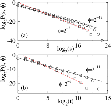
Figure 3: (Color online) (a) Distribution of avalanche size $P(s,\phi)$ is plotted in double logarithmic scale for two different values of $\phi$: $\phi=2^{-12}$ ($\Circle$) and $\phi=2^{-3}$ ($\Box$). Straight lines are fitted through data points. The slope of the solid black line is $-1.11\pm 0.01$ and that of the dashed red line is $-1.50\pm 0.01$. (b) Plot of $P(t,\phi)$ against $t$. The slope of the solid black line is $-1.18\pm 0.01$ and the dashed red line has slope $-1.98\pm 0.02$.

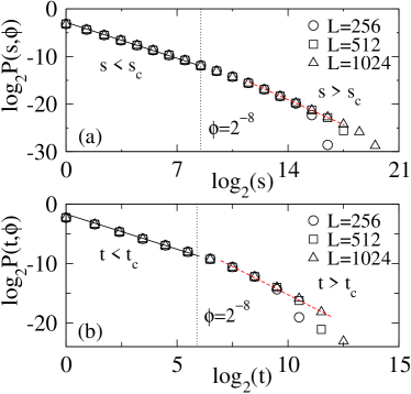
Figure 4: (Color online) (a) Distribution of avalanche size $P(s,\phi)$ is plotted in double logarithmic scale for $\phi=2^{-8}$ for three different system size $L=256$($\Circle$), $512$($\Box$), $1024$($\triangle$). Vertical dotted line at $s=s_{c}$ seperates the two regimes. The slope of the solid black line for $s<s_{c}$ is $-1.11\pm 0.01$ and that of the dashed red line for $s>s_{c}$ is $-1.50\pm 0.01$. (b) Plot of $P(t,\phi)$ versus $t$. Vertical dotted line at $t=t_{c}$ seperates the two regimes. The black solid line for $t<t_{c}$ has the slope $-1.18\pm 0.01$ and red dashed line for $t>t_{c}$ has slope $-1.98\pm 0.02$.

Figure 5: The values of the exponent $\tau_{s}(\phi)$ against $\phi$ are given in (a) and that of $\tau_{t}(\phi)$ against $\phi$ are given in (b). The extrapolated dashed lines indicate possible exponent values for larger system sizes.

In order to estimate the probability distributions of the avalanche properties and their conditional expection values, the following statistical averages are made. Sixteen SWNs configurations are considered for a given $\phi$. On each SWN, after attaining the steady state $10^{6}$ avalanches are neglected and next $2\times 10^{6}$ avalanches are collected. Therefore, a total of $32\times 10^{6}$ avalanches are taken for data averaging. The value of $\phi$ is varied from $0$ to $1$ increasing $N_{\phi}$ in multiple of $2$. The values of $\tau_{x}(\phi)$ are estimated determining the probability distributions of the respective avalanche properties $x\in\{s,a,t\}$.

Probability distributions of avalanche size $P(s,\phi)$ and that of lifetime $P(t,\phi)$ are estimated on SWNs generated for different values of $\phi$ for a given lattice size. For $\phi=2^{-12}$ (close to $\phi=0$) and $\phi=2^{-3}$ (close to $\phi=1$), $P(s,\phi)$ and $P(t,\phi)$ obtained on a lattice of size $L=1024$ are plotted in Fig.3(a) and Fig.3(b) respectively. It can be seen that for both $\phi=2^{-12}$ as well as for $\phi=2^{-3}$, $P(s,\phi)$ and $P(t,\phi)$ have power law behavior almost over the whole extent of $s$ and $t$ but with different critical exponents. The scaling behavior at $\phi=2^{-12}$ is found to be characterized by the avalanche size exponent $\tau_{s}=1.11\pm 0.01$, and avalanche time exponent $\tau_{t}=1.18\pm 0.01$, which are measured by the best fitted straight line (black) through the data points. The value of $\tau_{s}$ for $\phi=2^{-12}$ is same as that of previously reported for DSM on RL ($\phi=0$) shilo ; malcai . Note that the value of $\tau_{s}$ of the BTW model (Dhar abelian sandpile model dhar_rev ) was also reported to be $\approx 1.11$ though in the $L\rightarrow\infty$ limit it is expected to be $\approx 1.29$ solomon ; lubeck ; lubeck_ex . Therefore the BTW type sandpile dynamics on RL remains unperturbed when performed on a lattice with additional $N_{\phi}=512$ shortcuts corresponding to $\phi=2^{-12}$ on a lattice of size $L=1024$. On the other hand, the power law scaling at $\phi=2^{-3}$ is found to be characterized by a critical exponents $\tau_{s}=1.5\pm 0.01$ and $\tau_{t}=1.98\pm 0.02$. The value of $\tau_{s}$ for DSM obtained by mean field (MF) theory for lattices without spatial structure chris as well as by branching process for RN chris ; ebon was known to be $3/2$ and the exact value of $\tau_{t}$ on RN obtained by branching process is $2$ ebon . Hence, the measured value of $\tau_{t}=1.98$ for RN is close to the exact result. Therefore by the addition of $N_{\phi}=2^{18}$ shortcuts corresponding to $\phi=2^{-3}$ on a lattice of size $L=1024$, the RL evolves to a RN and DSM scaling on it can be described by MF scaling though the critical height is not taken as the mean degree of nodes as it was taken in Ref.chris .

For $\phi=2^{-8}$ (an intermidiate value of $\phi$), $P(s,\phi)$ and $P(t,\phi)$ are plotted in Fig.4(a) and Fig.4(b) respectively for different values of system size $L$. It is interesting to note that for $\phi=2^{-8}$, the distributions of $P(s,\phi)$ and $P(t,\phi)$ follow two different power law scaling at different regimes of $s$ and $t$ respectively, separated by a characteristic value $s_{c}$ and $t_{c}$ as shown by dotted lines in Fig.4(a) and Fig.4(b). The values of $s_{c}$ and $t_{c}$ are obtained from Eq.15 and Eq.16 respectively. For $s<s_{c}$, the scaling behavior of $P(s,\phi)$ is characterized by $\tau_{s}=1.11\pm 0.01$ whereas for $s>s_{c}$ it is characterized by $\tau_{s}=1.5\pm 0.01$. Therefore for SWNs corresponding to intermediate values of $\phi$, both the scaling forms, BTW and MF, of DSM coexist. It should also be noticed that the characteristic size $s_{c}$ or characteristic time $t_{c}$ does not change with system size $L$, as the characteristic length scale $\xi$ does not depend on $L$ newman . The values of the critical exponent $\tau_{s}(\phi)$ and $\tau_{t}(\phi)$ obtained for different values of $\phi$ are given in Fig.5(a) and Fig.5(b). It is important to note that coexistence of both the scaling forms persists over a wide range of $\phi$ given by $2^{-12}<\phi<2^{-3}$ for $s$ and $2^{-11}<\phi<2^{-3}$ for $t$. The upper limit corresponds to crossover of SWN to RN at $\phi\approx 0.1$ newman_book2 . Though the crossover from RL to SWN occurs at $\phi\approx 1/L^{2}$ newman , for the finite system of size $L=1024$ the sandpile dynamics is able to recognize such a crossover only at $\phi=2^{-12}$ (or $\sim 10^{-4}$). If the system size increases, such crossover is expected to appear in the sandpile dynamics for smaller values of $\phi$ and both exponents would be possible to measure in this regime as shown by a dashed line in Fig.3(c). The avalanche area $a$ also displays a similar co-existence of scaling behavior over the same range of $\phi$. For RL, $\tau_{a}$ is found $1.12$ as per the reported value for the BTW model for finite systems lubeck_ex . However for RN, it is found that the value of $\tau_{a}=1.5$ as that of $\tau_{s}$ on RN. In the SWN regime, both the scaling forms are found to coexist.

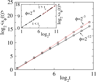
Figure 6: (Color online) Plot of $\langle s_{\phi}(t)\rangle$ against $t$ for $\phi=2^{-12}$ ($\circ$) and $\phi=2^{-3}$ ($\Box$). Solid lines are the best fitted straight lines having slope $1.62\pm 0.02$ (black solid line) for $\phi=2^{-12}$ and $1.98\pm 0.03$ (red dashed line) for $\phi=2^{-3}$. In the inset $\langle s(t)\rangle$ against $t$ for $\phi=2^{-8}$ is plotted.

The coexistance of scaling is also verified for the condiotional expectation value $\langle s_{\phi}(t)\rangle$. Its variation against $t$ for $\phi=2^{-12}$ and $2^{-3}$ are shown in Fig.6. The critical exponent $\gamma_{st}$ are obtained as $1.62\pm 0.02$ and $1.98\pm 0.03$ for $\phi=2^{-12}$ and $\phi=2^{-3}$ respectively. Since on RL $\tau_{s}=1.11$ and $\tau_{t}=1.18$, the expected value of $\gamma_{st}$ from the scaling relation Eq.13 is $1.63$ on RL. Similarly for RN, $\tau_{s}=1.5$ and $\tau_{t}=2$, the expected values of $\gamma_{st}=2$ on RN. The values of the critical exponents $\gamma_{st}$ are within the error bars of the expected values. In the inset of Fig.6, $\langle s(t)\rangle$ is plotted against $t$ for $\phi=2^{-8}$. Two different scaling of $\langle s_{\phi}(t)\rangle$ with $t$ are shown by back solid line and red dashed line respectively for $t<t_{c}$ and $t>t_{c}$. The coexistence scaling of $\langle s_{\phi}(t)\rangle$ is also observed for the same range of $\phi$ as it was observed for the avalanche size distribution.

It could be recalled that in an SWN there exists the concept of neighborhood corresponding to RL at the same time the shortest distance $\ell$ between two nodes is vanishingly small corresponding to RN. Because of the coexistence of both the characteristics of RL as well as that of RN in an SWN, the sandpile avalanches are segregated according to their sizes into two scaling forms. It should be emphasized here that such coexistence of two scaling behaviors is also observed on SWNs generated by removing the bonds emanating from a site of a square lattice with probability $\phi$ and rewiring it to a randomly selected lattice site. However, in contrary to the present observation, Arcangelis and Hermann herrmann obtained a continuous crossover from BTW universality class to MF universality class in the study of a BTW type sandpile dynamics on SWNs constructed by rewiring a fraction of bond of a square lattice keeping the critical height same for all the nodes and having dissipation only at the lattice boundary. No coexisting region of both the scaling forms was observed in their study. On the other hand, in the study of one dimensional sandpile model on SWNs a transition from non-critical to critical regime was demonstrated by Lahtinen et al. kaski .

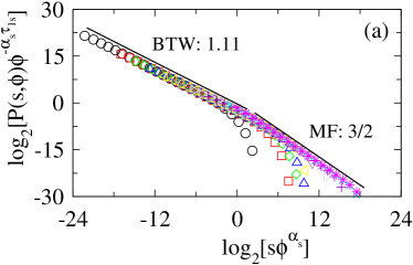
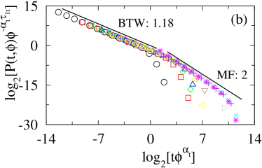
Figure 7: (Color online) (a) Plot of scaled distribution $P(s,\phi)\phi^{-\alpha_{s}\tau_{1s}}$ against a scaled variable $z_{s}=s\phi^{\alpha_{s}}$. (b) Plot of $P(t,\phi)\phi^{-\alpha_{t}\tau_{1t}}$ against $z_{t}=t\phi^{\alpha_{t}}$. Different symbols corresponding to different $\phi$ values are taken as: $\phi=2^{-21}(\Circle)$, $2^{-16}(\Box)$, $2^{-14}(\Diamond)$, $2^{-12}(\triangle)$,$2^{-10}(\triangleleft)$, $2^{-8}(\triangledown)$, $2^{-6}(\triangleright)$, $2^{-4}(+),2^{-1}(\times)$, $2^{0}(\hexstar)$. Reasonable data collapse for both $s$ and $t$ are observed. Solid lines with respective slopes are guide to eye.

VI Scaling of coexisting probability distributions

As per the scaling form of the characteristic toppling area $a_{c}$, size $s_{c}$, lifetime $t_{c}$ (obtained in Eqs.14,15 and 16 respectively), a general scaling of the charateristic property $x_{c}$ with $\phi$ is assumed as

$$x_{c}(\phi)\approx\phi^{-\alpha_{x}}$$ (17)

where $\alpha_{x}$s correspond to different characteristic exponents. The values of $x_{c}(\phi)$ on RL ($\phi=0$), must correspond to the cut off value of the distribution $P(x,0)$ for a given system size $L$. As the network grows, the distribution $P(x,\phi)$ will develop a part corresponding to MF scaling. Consequently the part representing the BTW type scaling will shrink. Hence, the value of $x_{c}$ should decrease with increasing $\phi$. Eventually, the value of $x_{c}$ will be the one on RN when $\phi=1$. The existence of such a characteristic value of toppling size as a function of was noticed in the sandpile dynamics on one dimensional SWN kaski . It is now possible to obtain a single probability distribution function for both the scaling forms for the whole range of $\phi$.

A new scaling form for the distribution functions with respect to the characteristic value $x_{c}(\phi)$ is now proposed as

$$P(x,x_{c}(\phi))=\left\{\begin{array}[]{ll}x^{-\tau_{1x}}{\sf f}\left(\frac{x}{x_{c}(\phi)}\right)&\mbox{for $x\leqslant x_{c}$}\\ x^{-\tau_{2x}}{\sf g}\left(\frac{x}{x_{c}(\phi)}\right)&\mbox{for $x\geqslant x_{c}$ }\end{array}\right.$$ (18)

where ${\sf f}$ and ${\sf g}$ are two different scaling functions in two different regions and $\tau_{1x}$ and $\tau_{2x}$ are the corresponding critical exponents in the respective regions. Since at $x=x_{c}(\phi)$ the values of $P(x,x_{c}(\phi))$ are same for both the regions, then one should have ${\sf f}(1)=\phi^{-(\tau_{1x}-\tau_{2x})\alpha_{x}}{\sf g}(1)$. The probability distribution then can be obtained in terms of a single scaling function ${\sf f}$ or ${\sf g}$ as

$$P(x,\phi) = \left\{\begin{array}[]{ll}x^{-\tau_{1x}}{\sf f}(x\phi^{\alpha_{x}})&\mbox{for $x\leqslant x_{c}$}\\ x^{-\tau_{2x}}\phi^{-\Delta_{x}\alpha_{x}}{\sf f}(x\phi^{\alpha_{x}})&\mbox{for $x\geqslant x_{c}$ }\\ \end{array}\right.$$ (21)

where $\Delta_{x}=(\tau_{2x}-\tau_{1x})$. The $\phi$ independent scaling form can be obtained by rescaling the probability distribution as

$$P(x,\phi)\phi^{-\alpha_{x}\tau_{1x}} = \left\{\begin{array}[]{ll}z_{x}^{-\tau_{1x}}{\sf f}(z_{x})&\mbox{for $z_{x}\leqslant 1$}\\ z_{x}^{-\tau_{2x}}{\sf f}(z_{x})&\mbox{for $z_{x}\geqslant 1$ }\\ \end{array}\right.$$ (24)

where $z_{x}=x\phi^{\alpha_{x}}$ is a scaled variable. Such scaling behavior was also observed in context of anomalous roughening of fractured surface lopez .

The above scaling forms are now verified. The rescaled probabilities $P(x,\phi)\phi^{-\alpha_{x}\tau_{1x}}$ are plotted against the scaled variable $z_{x}=x\phi^{\alpha_{x}}$ for $s$ and $t$ in Fig.7(a) and (b) respectively. It can be seen that a good data collapse is obtained for both $s$ and $t$ using $\alpha_{s}=1.06$ and $\alpha_{t}=0.65$. The critical exponents $\tau_{x}$ corresponding to two different regions are also verified. The straight lines with required slopes in the respective regions are guide to eye. It confirms the proposed scaling form of the probability distribution functions on SWNs. Such coexistence scaling in the SWN regime is also verified for a stochastic sandpile model ssm .

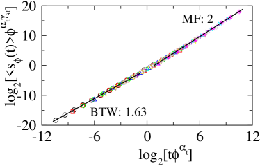
Figure 8: (Color online) Plot of $\langle s_{\phi}(t)\rangle\phi^{\alpha_{t}\gamma_{st}}$ against a scaled variable $t\phi^{\alpha_{t}}$. The same symbol set of Fig.7 is used. A good data collapse is observed. Two solid lines having slopes $1.63$ and $2$ indicating two different scaling forms are guide to eye.

Since the probability distributions are now represented by a single scaling form, the average avalanche properties can also be scaled in a similar fashion. For example, the average cluster size is now expected to scale as

$$\langle s_{\phi}(t)\rangle=t^{\gamma_{st}}f_{st}(t\phi^{\alpha_{t}})$$ (25)

where $f_{st}$ is a new scaling function and the value of $\gamma_{st}$ correspond to that on RL. The form of the scaling function is verified by plotting $\langle s_{\phi}(t)\rangle\phi^{\gamma_{st}\alpha_{t}}$ against the scaled variable $t\phi^{\alpha_{t}}$ in Fig.8 taking $\gamma_{st}=1.63$. It can be seen that there is a good data collapse and the scaling function represents two different scaling behaviors with two different exponents as $1.63$ and $2$, indicated by straight lines with respective slopes. Such scaling behavior can also be obtained between avalanche size $s$ and area $a$. Since $\alpha_{a}=1$ and $\gamma_{sa}=1.06$, the change in slope in the scaling function is difficult to observe in the numerical data collected here.

It is now important to understand the origin of coexistence of both the critical behaviors of the avalanche properties on an SWN. Since for an avalanche property $x$ there is BTW type scaling for $x<x_{c}$ and MF type scaling for $x>x_{c}$, it is intriguing to look into the avalanche cluster morphology for the avalanches following two different scaling behaviors.

VII Avalanche cluster morphology

Morphology of avalanche clusters obtained in the steady state of DSM on SWNs corresponding to different $\phi$ values are shown in Fig.9. These avalanches are obtained on SWNs defined on a square lattice of size $512\times 512$ for $\phi=2^{-12}$, $\phi=2^{-8}$ and $\phi=2^{-3}$. Different colors correspond to different numbers of toppling of a node. A typical avalanche cluster in the RL regime with $\phi=2^{-12}$, is shown in Fig.9(a). The avalanche cluster (of size $s=63774$) is isotropic and mostly compact. It consists of concentric zones of lower and lower number of toppling around the node with maximum number of toppling (in purple) as expected for a BTW type avalanche cluster grass ; chris . Few clusters of compact structure appear here and there because of the presence of a small number of shortcuts in the system a few sands grains are transported to the remote parts of the lattice. However such a small distortion in the morphology of avalanche cluster with respect to a single compact BTW type cluster is not able to modify the scaling behavior.

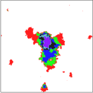
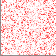
(a) $\phi=2^{-12}$ (b) $\phi=2^{-3}$

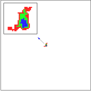
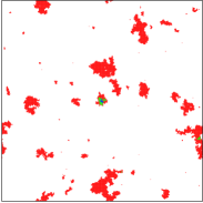
(c) $\phi=2^{-8}$, $(s<s_{c})$ (d) $\phi=2^{-8}$, $(s>s_{c})$

Figure 9: (Color online) Morphology of avalanche clusters of DSM on SWN generated on $L=512$ square lattice for different values of $\phi$. (a) For $\phi=2^{-12}$, almost a BTW type cluster. (b) For $\phi=2^{-3}$, avalanche cluster on a RN completely scattered all over the lattice. (c) For $\phi=2^{-8}$, a small avalanche cluster of size ($352$) less than $s_{c}(\approx 360)$ is shown. Enlarged version of the same avalanche cluster is given in the inset. (d) For $\phi=2^{-8}$, a large avalanche cluster (a different realization than (c)) of size ($16872$) greater than $s_{c}$. Different colors correspond to different numbers of toppling of a node: red for $1$, green for $2$, blue for $3$, black for $4$, skyblue for $5$ and purple for more than $5$ toppling. No color corresponds to the nodes that did not topple at all during the avalanche. The black border represents the lattice boundary.

In Fig.9(b), a typical avalanche cluster ($s=33567$) obtained on RN corresponding to $\phi=2^{-3}$ is shown. In this case, the avalanche cluster is completely scattered all over the network. A large number of shortcuts are added to RL to make it RN and hence sand grains from a toppled node of RN are transported to almost all other nodes of the network through the shortcuts. The compact BTW type cluster is therefore found scattered all over the lattice or the network. Small patches of sites toppled only once are still present. As $\phi$ approaches $1$, the size of such patches reduces.

The morphology of avalanche cluster of DSM on SWN with intermediate $\phi$ is found either as that of BTW type cluster on RL or as sparse clusters on RN. Two such avalanche clusters on SWN with $\phi=2^{-8}$ are shown in Fig.9(c) and (d). It is already seen that the avalanche clusters on SWNs with intermediate $\phi$ follow two different scaling forms below and above a characteristic toppling size $s_{c}$. For $\phi=2^{-8}$, it is given by $s_{c}=\phi^{-1.06}\approx 360$. A cluster of size $352$ ($<s_{c}$) is shown in Fig.9(c) and a cluster of size $16872$ ($>s_{c}$) is shown in Fig.9(d). The larger cluster in Fig.9(d) is broken into patches consisting of nodes mostly toppled once and scattered over most of the network whereas the smaller cluster in Fig.9(c) is still isotropic and compact. An enlarged version of the small cluster is shown in the inset of Fig.9(c). Therefore, on an SWN two types of clusters appear. The smaller compact clusters ($s<s_{c}$) naturally follow BTW type scaling and the large sparse clusters ($s>s_{c}$) follow MF type scaling. The coexistence of two scaling forms on an SWN is then due to the presence of both the clusters on the same network. As $\phi$ decreases (goes toward RL), $s_{c}$ becomes larger and consequently all clusters are of BTW type. On the other hand as $\phi$ increases to $1$ (RN), $s_{c}$ goes down to $1$ and all the clusters are sparse and scattered over all the nodes.

Sandpile dynamics then can be used as an useful tool to probe different length scales present in the underlying structure on which it is performed. The avalanches are expected to display appropriate scaling behavior corresponding to different length scales.

VIII Distribution of area of various toppling sites

Figure 10: Plot of $P(a,\phi)$ and $P(a_{n},\phi)$ for $n=1,2,3$ in double logarithmic scale for different values of $\phi$: For $\phi=0$ (a), $\phi=2^{-8}$ (b) and $\phi=1$ (c) for the system size $L=1024$.

From the morphologies of avalanche clusters, it is seen that on RL the avalanches are consisting of sites toppled multiple times whereas on RN they are mostly consisting of nodes toppled only once. On SWN with intermediate $\phi$, clusters of both types appear. In order to understand the type of sites present in an avalanche, the distribution of area $a_{n}$ of sites those are toppled a fixed $n$ number of times should be analyzed. Such area distributions for BTW model on RL were found to obey power law scaling with exponents close to that of the total area distribution exponent dhar_mann ; banerjee . The idea of studying distributions of $a_{n}$ is extended here to the avalanches obtained on SWNs. The scaling behavior of number of sites or nodes that toppled $n$-times is then assumed to be

$$P(a_{n},\phi)\approx a_{n}^{-\tau_{a}^{(n)}(\phi)}$$ (26)

where $n=1,2,3,\cdots$ corresponding to sites toppled only once, only twice, only thrice, etc. In Fig.10, distribution functions $P(a_{n},\phi)$ corresponding to only once ($a_{1}$), only twice ($a_{2}$), only thrice ($a_{3}$) are plotted and compared with the distribution of total area $a$ for three different values of $\phi$, (a) $\phi=0$, (b) $\phi=2^{-8}$ and (c) $\phi=1$ for $L=1024$. On RL, all three distributions are extended over a long range of $a_{n}$, almost as large as total area $a$. The distribution of $a_{1}$ has an exponent $\tau_{a}^{(1)}=1.12\pm 0.01$ same as $\tau_{a}$. As the network grows to an intermediate regime, say for $\phi=2^{-8}$, the distributions of $a$ and $a_{1}$ are found to be almost same for all values of area as given in Fig.10(b) whereas the distributions of $a_{2}$ and $a_{3}$ are shrunk toward smaller areas. It can also be noticed that the distribution of $a$ or $a_{1}$ has two different scaling forms corresponding to two different regimes as it is seen in the case of distribution of $s$ and $t$ (Fig.4(a), Fig.4(b)). For $\phi=1$, the distribution of $a_{1}$ and that of $a$ become inseparable as shown in Fig.10(c) and they have same distribution exponent $\approx 1.5$ as that of the avalanche size $s$ on a RN. This means that the avalanches are consisting of singly toppled nodes and the difference between the avalanche area $a$ and avalanche size $s$ disappears. The distribution of $a_{2}$ reduces to a point and there is no node that toppled thrice or more. It can be noted that $a_{2}=1$, i.e.; only one node has toppled twice. The probability of occurrence of such an event is also very small, $P(a_{2},\phi=1)\approx 1/2^{20}$. It had already been noted that the possibility of formation of loop in a branching process of toppling events on a RN is vanishingly small and usually goes as $1/L^{2}$, inverse of the number of nodes chris ; ebon . Thus the present observation is consistent with the prediction of branching process.

Figure 11: Plot of $\langle(a/s)_{\phi}\rangle$ ($\Circle$) and $\langle(a_{1}/a)_{\phi}\rangle$ ($\Box$) against $\phi$ for the system size $L=1024$.

Not only the probability distributions of $a$ and $s$ are same but also the magnitude of $a$ and $s$ are found to be same on RN. This is verified by calculating the ratio $\langle(a/s)_{\phi}\rangle$ and $\langle(a_{1}/a)_{\phi}\rangle$ for several values of $\phi$. The variation of $\langle(a/s)_{\phi}\rangle$ against $\phi$ is shown in Fig.11 and compare with that of $\langle(a_{1}/a)_{\phi}\rangle$. It can be seen that for $\phi\geq 0.1$ both the ratios are one. They decrease as $\phi$ decreases. For $\phi<0.1$, the ratio $\langle(a/s)_{\phi}\rangle<1$ indicates that $s>a$ and the ratio $\langle(a_{1}/a)_{\phi}\rangle<1$ indicates that $a>a_{1}$. It can also be noted that $\langle(a/s)_{\phi}\rangle$ and $\langle(a_{1}/a)_{\phi}\rangle$ are same for $\phi\geq 0.1$ whereas for $\phi<0.1$ they are different.

IX Time autocorrelation of toppling waves

A toppling wave is the number of toppling during the propagation of an avalanche starting from a critical site without toppling the same site further. Each toppling of the critical site creates a new toppling wave. The total number of toppling $s$ in an avalanche can be considered as

$$s=\sum_{k=1}^{m}s_{k}$$ (27)

where $s_{k}$ is the number of toppling in the $k$th wave and $m$ is the number of toppling waves in an avalanche. The time evolution of toppling dynamics then can be studied coarsening the avalanches into a series of toppling waves prie . The toppling waves generated in the BTW model on RL were found to be correlated menech_corr . As a consequence of such correlation in the toppling waves, it was observed that the model does not obey finite size scaling (FSS) karmakar . It is then interesting to study the time autocorrelation of the toppling waves for DSM on SWNs to get a limiting value of $\phi$ at which FSS would be obeyed for this model. Following Menech and Stella menech_corr , a time autocorrelation function for an SWN with given $\phi$ is defined as

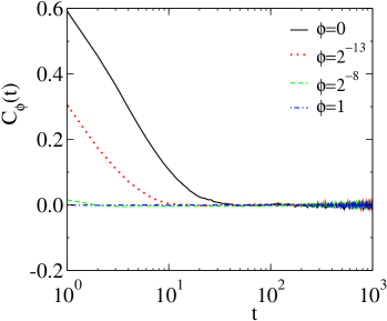
Figure 12: Plot of $C_{\phi}(t)$ against $t$ for different values of $\phi$: $\phi=0$ (in black solid line), $\phi=2^{-13}$ (in red dotted line), $\phi=2^{-8}$ (in green dashed line), and $\phi=1$ (in blue dashed dotted line) for $L=1024$.

$$C_{\phi}(t)=\frac{\langle s_{k+t}s_{k}\rangle-\langle s_{k}\rangle^{2}}{\langle s_{k}^{2}\rangle-\langle s_{k}\rangle^{2}}$$ (28)

where $t=1,2,\cdots$ and $\langle\cdots\rangle$ represents the time average. $C_{\phi}(t)$ is calculated for four different values of $\phi$, $\phi=0$, $\phi=2^{-13}$, $\phi=2^{-8}$ and $\phi=1$ on a system of size $L=1024$, generating $2\times 10^{6}$ toppling waves in the steady state for each $\phi$. $C_{\phi}(t)$s obtained for the above $\phi$ values are plotted against $t$ in Fig.12. It can be seen that the toppling waves in DSM on the original lattice ($\phi=0$) is positive (shown by a black solid line) and hence highly correlated. Whereas on RN ($\phi=1$) it is always zero and hence completely uncorrelated (shown by a blue dashed dotted line). As $\phi$ increases from $0$ to $1$, the strength of positive correlation decreases and vanishes at $\phi\approx 0.1$ corresponding to the onset of RN. Zero autocorrelation in the toppling waves on RN is consistent with the fact that the avalanches on such a network are consisting of nodes mostly toppled only once. Since almost no node in an avalanche toppled twice, an avalanche is then represented by a single toppling wave. The toppling wave time series then consists of sequence of toppling numbers of a single toppling wave of independent avalanches. Hence, the toppling waves become uncorrelated. On the other hand, the toppling waves of DSM on RL remain correlated as in the case of BTW. It should be emphasized here that Karmakar et al. karmakar had shown that the toppling wave correlation in BTW type sandpile model on a RL is essentially due to precise toppling balance. Though in the present model on RN precise toppling balance is present in the toppling rule, the toppling waves become uncorrelated. Because on RN, the probability of formation of loop in the toppling sequence is vanishingly small and hence the concept of precise toppling balance become ineffective.

Since an avalanche cluster on RN consists of a single toppling wave, the feedback to the original toppled node remains so low that in most of the cases it never become upper critical again. Hence, in the context of information propagation, the critical RN behaves like a one way network. May be due to the fact that the RN already behaves like a one way network, the sandpile on directed small world network he is found to belong to the same MF universality class.

X Diffusive to super diffusive sand transport

The critical behavior of sandpile models on RL is believed to be governed by the diffusive sand transport during avalanches. Since the avalanche size (the total number of toppling) is equivalent to the number of steps of a random walker starting from an arbitrary site to reach the lattice boundary of a RL shilo ; ssms , their scaling behavior with lattice size (or number of nodes) on SWNs is now important to characterize. For a given $\phi$ and system size $L$, the average number of steps $\langle n_{\phi}(L)\rangle$ required for a random walker to reach the lattice boundary starting from an arbitrary node of an SWN and the average avalanche size can be defined as

$$\langle n_{\phi}(L)\rangle=\int_{0}^{n_{max}}nP_{\phi}(n,L)dn$$ (29)

and

$$\langle s_{\phi}(L)\rangle=\int_{0}^{s_{max}}sP_{\phi}(s,L)ds$$ (30)

where $P_{\phi}(n,L)$ is the probability to find a random walk with $n$ steps that reaches the lattice boundary starting from an arbitrary node and $P_{\phi}(s,L)$ is the probability to have an avalanche of size $s$ for the given $\phi$ and $L$. The scaling of $\langle n_{\phi}(L)\rangle$ and $\langle s_{\phi}(L)\rangle$ with $L$ is assumed to be

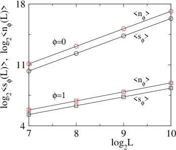
Figure 13: (Color online) Average avalanche size $\langle s_{\phi}(L)\rangle$ (symbols in black) and $\langle n_{\phi}(L)\rangle$ (symbols in red) is plotted against system size $L$ for $\phi=0$ ($\Circle$) and $\phi=1$ ($\Box$). Solid line through the circles has slope $2$ and that through the squares has slope $1$.

$$\langle n_{\phi}(L)\rangle\sim L^{\sigma_{n}(\phi)}\hskip 14.22636pt\mbox{and}\hskip 14.22636pt\langle s_{\phi}(L)\rangle=L^{\sigma_{s}(\phi)}$$ (31)

where $\sigma_{n}(\phi)$ and $\sigma_{s}(\phi)$ are two exponents. In order to verify such a scaling forms for $\langle n_{\phi}(L)\rangle$ and $\langle s_{\phi}(L)\rangle$, they are estimated as a function of $L$ for $\phi=0$ and $\phi=1$. In Fig.13, $\langle n_{\phi}(L)\rangle$ and $\langle s_{\phi}(L)\rangle$ are plotted against $L$ in double logarithmic scale for both the values of $\phi$. The values of the exponents $\sigma_{n}(\phi)$ and $\sigma_{s}(\phi)$ are obtained as $\sigma_{n}=\sigma_{s}\approx 2$ for $\phi=0$ and $\sigma_{n}=\sigma_{s}\approx 1$ for $\phi=1$. The solid lines are guide to eye with respective slopes. Since at $\phi=0$, both $\langle n_{\phi}(L)\rangle$ and $\langle s_{\phi}(L)\rangle$ scale as $\sim L^{2}$, the random walk or the sand transport both are of diffusive nature whereas at $\phi=1$ they scale as $\sim L$, therefore they are of super diffusive nature. It is observed that the super diffusive nature sustains over the whole RN region $\phi\geq 0.1$. But the diffusive nature quickly dies out as the number of shortcuts increases in the system. For intermediate values of $0<\phi<0.1$, no definite values of $\sigma_{n}(\phi)$ or $\sigma_{s}(\phi)$ was possible to estimate because the data did not represent a linear relationship on double logarithmic scale. The curvature in the data is due to the fact that in the intermediate region of $\phi$ both the scaling forms of $P(s,\phi)$ coexists. Therefore a crossover from diffusive to super diffusive sand transport occurs as RL is evolved to RN. It can be seen that not only the scaling of $\langle n_{\phi}\rangle$ and $\langle s_{\phi}\rangle$ are same but also the magnitude of $\langle n_{\phi}\rangle$ is just twice of $\langle s_{\phi}\rangle$ for both $\phi=0$ and $\phi=1$ on a given $L$. On RL it was already known that $\langle n_{\phi}\rangle=2\langle s_{\phi}\rangle$ malcai ; shilo . Such a relationship is then also valid on RN. It is also interesting to note that the absolute values of $\langle s_{\phi}\rangle$ (or $\langle n_{\phi}\rangle$) is much smaller on RN than on RL for a given $L$. It could be recalled that the avalanches on RN consist of nodes that toppled only once whereas on RL there exist sites that toppled multiple times. The cut off of the distribution $P(s,\phi)$ on RN is much smaller than that on RL (see Fig.3). Therefore, on RN occurrence of an avalanche cluster with nodes toppled only ones, consists of a single toppling wave, super diffusive sand transport during an avalanche all are inter connected phenomena.

Since the shortest distance $\ell$ between two nodes of an SWN follows two different scaling behavior given in Eq.1 and 4, it would be interesting to verify whether $\langle n_{\phi}(L)\rangle$ and $\langle s_{\phi}(L)\rangle$ follow a similar scaling behavior on SWN or not. Following the scaling of $\langle\ell\rangle$ given in Eq.4, general scaling forms of $\langle n_{\phi}(L)\rangle$ and $\langle s_{\phi}(L)\rangle$ are proposed as

$$\langle n_{\phi}(L)\rangle=L^{2}\mathcal{G}(\phi^{1/2}L)$$ (32)

and

$$\langle s_{\phi}(L)\rangle=\frac{1}{2}L^{2}\mathcal{G}(\phi^{1/2}L)$$ (33)

where $\mathcal{G}(x)$ is a universal scaling function given by

$$\mathcal{G}(x) \propto \left\{\begin{array}[]{ll}\mbox{constant,}&x\ll 1\\ 1/x,&x\gg 1\\ \end{array}\right.$$ (36)

Verification of the above scaling form is performed by estimating $\langle n_{\phi}(L)\rangle$ and $\langle s_{\phi}(L)\rangle$ for different $L$ for the whole range of $\phi$ between $0$ and $1$. In Fig.14, $\langle n_{\phi}(L)/L^{2}\rangle$ and $2\langle s_{\phi}(L)\rangle/L^{2}$ are plotted against the scaled variable $x=\phi^{1/2}L$. Reasonable data collapses are observed for both $\langle n_{\phi}(L)\rangle$ and $\langle s_{\phi}(L)\rangle$. It should be noted here that on a two dimensional regular square lattice $\langle n_{\phi}\rangle\approx aL+bL^{2}$, where $a=0.56$ and $b=0.14$ for small $L$ shilo . However in the limit $L\rightarrow\infty$, such a scaling can be approximated as $\langle n_{\phi}(L)\rangle\approx 0.14L^{2}$. In the limit $\phi\rightarrow 0$, the scaling function approaches $0.14$. On the other hand, the $1/x$ scaling would be valid on RN, i.e. for $\phi\geq 0.1$. For the lowest lattice size the corresponding value of the scaled variable is marked by a cross on the horizontal axis beyond which $1/x$ scaling is expected to be valid. It should also be noted here that the number of distinct nodes $S(n)$ visited by a random walker in $n$ time steps on a $1d$ SWN for a fixed $L$ and $\phi$ represents a crossover in scaling from $S(n)\sim\sqrt{n}$ for $n\ll\xi^{2}$ to $S(n)\propto n$ for $n\gg\xi^{2}$ jasch ; lahtinen ; almaas .

Figure 14: Plot of $2\langle s_{\phi}(L)\rangle/L^{2}$ and $\langle n_{\phi}(L)\rangle/L^{2}$ against the scaled variable $\phi^{1/2}L$. Different symbols for $\langle s_{\phi}(L)\rangle$ for different system size are: $\Circle$ for $L=256$, $\Box$ for $512$ and $\Diamond$ for $1024$. For $\langle n_{\phi}(L)\rangle$ they are: $\triangle$ for $L=256$, $\triangleleft$ for $512$ and $\triangleright$ for $1024$. A reasonable data collapse is observed.

XI FSS on random network

Since SWNs are generated on finite systems of size $L$ with a given $\phi$, the probability distributions of avalanche quantities then should depend on $L$. The scaling form of the distribution function is assumed to be

$$P_{\phi}(x,L)=x^{-\tau_{x}(\phi)}f[x/L^{D_{x}(\phi)}]$$ (37)

where $x\in\{s,a,t\}$ and $D_{x}(\phi)$ is the capacity dimension of the avalanche property $x$ on SWN with a given $\phi$. It was observed that the avalanche properties like $s$ or $t$ of BTW type models do not follow FSS ansatz on RL menech_moment ; lubeck . In the following, the FSS analysis is performed for $s$ and $t$ on RN as well as on SWNs employing moment analysis menech_moment ; lubeck ; karmakar . The average $q$th moment of an avalanche property $x$ for a given $\phi$ can be obtained as

$$\langle x_{\phi}^{q}(L)\rangle = \int_{0}^{x_{max}}x^{q}P_{\phi}(x,L)dx$$ (38)

$$= \int_{0}^{x_{max}}x^{q-\tau(\phi)}f[x/L^{D_{x}(\phi)}]dx.$$

Hence, the system size dependence of $\langle s_{\phi}^{q}(L)\rangle$ and $\langle t_{\phi}^{q}(L)\rangle$ are expected to be

$$\langle s_{\phi}^{q}(L)\rangle\sim L^{\sigma_{s}(q,\phi)}\hskip 14.22636pt\mbox{and}\hskip 14.22636pt\langle t_{\phi}^{q}(L)\rangle\sim L^{\sigma_{t}(q,\phi)}$$ (39)

where,

$$\sigma_{x}(q,\phi)=[q+1-\tau_{x}(\phi)]D_{x}(\phi).$$ (40)

for $x\in{\{s,t\}}$ and $q=1$ corresponds to the average values of the respective avalanche properties such as $\langle s_{\phi}\rangle$, $\langle t_{\phi}\rangle$, etc. For $P_{\phi}(x,L)$ to obey FSS for a given $\phi$ value, the moment exponent $\sigma_{x}(q,\phi)$ should have a constant gap between two successive values of $q$, i.e.; $\sigma_{x}(q+1,\phi)-\sigma_{x}(q,\phi)=D_{x}(\phi)$ for the respective $\phi$ value. For avalanche properties it was usually found that the gap converge to the respective capacity dimension as $q\rightarrow\infty$. In order to determine $D_{s}(\phi)$ and $D_{t}(\phi)$, sequences of exponents $\sigma_{s}(q,\phi)$ and $\sigma_{t}(q,\phi)$ are obtained for $400$ equally spaced values of $q$ between $0$ and $4$ for several $\phi$ values. The constant gap between two successive $\sigma_{x}(q,\phi)$s is then verified by estimating the slope $\partial\sigma_{x}(q,\phi)/\partial q$ using finite difference method.

Figure 15: (a) $\sigma_{x}(q,\phi)$ with $x\in\{s,t\}$ is plotted against $q$ for $\phi=1$. (b) $\partial\sigma_{x}(q,\phi)/\partial q$ is plotted against $q$ for $\phi=1$. It converges to $2$ for $x=s$ and to $1$ for $x=t$.

For $\phi<0.1$, the finite differences $\partial\sigma_{s}(q,\phi)/\partial q$ and $\partial\sigma_{t}(q,\phi)/\partial q$ for both the sequences of $\sigma_{s}(q,\phi)$ and $\sigma_{t}(q,\phi)$ did not converge to any finite value upto $q=4$. Hence, $P_{\phi}(x,L)$, $x\in\{s,t\}$ does not follow FSS ansatz in the SWN regime. Note that on SWN both the scaling coexist. Since $P_{\phi}(x,L)$ for $x<x_{c}$ does not follow FSS, the distribution functions for the full range of $x$ is then expected not to follow FSS.

For $0.1\leq\phi\leq 1$, FSS is expected to be valid and it is verified for several values of $\phi$ in this region. Data for $\phi=1$ is presented below. The variation of $\sigma_{s}(q,\phi)$ and $\sigma_{t}(q,\phi)$ for $\phi=1$ are plotted against moment $q$ in Fig.15(a) and that of $\partial\sigma_{s}(q,\phi)/\partial q$ and $\partial\sigma_{t}(q,\phi)/\partial q$ against moment $q$ are shown in Fig.15(b). It can be seen that for $\phi=1$ the derivatives saturate to $D_{s}\approx 2$ and $D_{t}\approx 1$ for higher values of $q$. The value of $D_{s}$ for $\phi=1$ is expected to be $2$ because on RN all avalanches are constituted of sites toppled only once, that is to say the avalanche area and avalanche size have no difference. On the other hand, the value of $D_{t}$ for $\phi=1$ is expected to be $1$ because on RN all avalanches are constituted of single toppling wave, that is to say the number of parallel updates in a single toppling wave is proportional to the system size $L$ (see Fig.3(b)). On the RL it was known that $D_{s}/D_{t}=\gamma_{st}$. Such a scaling relation is also valid on RN. Since $D_{s}=2$ and $D_{t}=1$ for $\phi=1$, the value of $\gamma_{st}$ is expected to be two as it is estimated in section V. For $q=1$ and $\phi=1$, the scaling relations $\sigma_{s}=(2-\tau_{s})D_{s}$ and $\sigma_{t}=(2-\tau_{t})D_{t}$ are expected to be satisfied. Since $\tau_{s}=3/2$ and $D_{s}=2$ for $\phi=1$, the value of $\sigma_{s}$ must be one as measured on RN. Similarly, from the other scaling relation $\sigma_{t}$ for $q=1$ is expected to be zero because $\tau_{t}=2$. Numerically a small finite value of $\sigma_{t}$ for $q=1$ is estimated. However, for $q=2$, $\sigma_{t}=1$ as expected.

Figure 16: Plot of scaled distribution $P_{\phi}(x,L)L^{D_{x}\tau_{x}}$ against the scaled variable $x/L^{D_{x}}$ for $\phi=1$ in (a) for $x=s$ and in (b) for $x=t$. Different symbol correspond to different system size as $L=256(\Circle)$, $512(\Box)$ and $1024(\triangle)$. A reasonable data collapse is obtained for both $s$ and $t$.

Finally the scaling function forms of $P_{\phi}(s,L)$ and $P_{\phi}(t,L)$ for $\phi=1$ on RN are verified by data collapse. In Fig.16(a), the scaled probability distribution $P_{\phi}(s,L)L^{D_{s}\tau_{s}}$ for $\phi=1$ is plotting against the scaled variable $s/L^{D_{s}}$ taking $\tau_{s}=3/2$ and $D_{s}=2$ as for RN. In Fig.16(b), $P_{\phi}(t,L)L^{D_{t}\tau_{t}}$ for $\phi=1$ is plotting against the scaled variable $t/L^{D_{t}}$ taking $\tau_{t}=2$ and $D_{t}=1$ as for RN. It can be seen that a reasonable data collapse is obtained for RN generated on three different systems sizes $L=256,512$ and $1024$. The assumed FSS form of $P_{\phi}(x,L)$ on the RN is then rightly chosen. Therefore, FSS would be valid even for a sandpile model with deterministic and conservative toppling rules along with complete toppling balance if it is defined on a system in which concept of neighborhood does not exist and has long distance connectivity.

XII Conclusion

A generalized DSM is constructed and studied on SWNs. Apart from BTW type correlated scaling for $\phi\lesssim 2^{-12}$, two important characteristic features of DSM, one on SWN for $2^{-12}<\phi<0.1$ and the other on RN for $0.1\leq\phi\leq 1$ are identified and characterized. First, DSM on SWNs exhibits two scaling behaviors simultaneously. One is that of BTW type scaling on RL and the other is that of MF scaling on RN corresponding to existence of strong neighborhood as that of RL as well as vanishingly small shortest distance between two nodes as that of RN on an SWN. A characteristic value of every avalanche property was possible to identify around which coexistence scaling of probability distribution functions are proposed and numerically verified. The avalanche clusters following BTW scaling are compact BTW type clusters whereas those following MF scaling are sparse and scattered all over the network. Since avalanche clusters segregate as per the length scales of the SWN, sandpile dynamics can be used as a probe to identify different length scales present in the underlying structure on which it is performed. Second, FSS is found to be valid for DSM on RN in contrary to the fact that DSM does not follow FSS on RL or on SWN. The validity of FSS on RN for DSM is due to the fact that the avalanches on RN are consisting of nodes toppled only once. The probability of appearance of a node that toppled more than once is vanishingly small on RN as the number of nodes $N\rightarrow\infty$. As a consequence, precise toppling balance becomes ineffective as well as toppling waves become uncorrelated. Because of the presence of long distance connections, sand transport becomes super diffusive on RN though it was diffusive on RL. Super diffusive sand transport is found to be essential in order to satisfy finite size scaling relations. Therefore, BTW type correlated sandpile models would also follow FSS if they are studied on systems without spatial structure and have long distance connections.

XIII Acknowledgments

Financial assistance from DST, Government of India through project No. SR/S2/CMP-61/2008 is gratefully acknowledged.

References

- (1) R. Albert and A. L. Barabási, Rev. Mod. Phys. 74, 47 (2002); S. Boccaletti, V. Lotora, Y. Moreno, M. Chavez, and D. U. Hwang, Phys. Rep. 424, 175 (2006).
- (2) H. Jeong, B. Tombor, R. Albert, Z. N. Oltvai, and A. L. Barabási, Nature (London) 411, 41 (2000).
- (3) Anna Levina, J. Michael Herrmann, and Theo Geisel, Nature Phys. 3, 857-860 (2007).
- (4) M. Faloutsos, P. Faloutsos, and C. Faloutsos, Comput. Commun. Rev. 29, 251 (1999).
- (5) R. Albert, H. Jeong, and A. L. Barabási, Nature (London) 401, 130 (1999); L. A. Adamic and A. B. Hubermann, Science 287, 2115 (2000).
- (6) F. Liljeros, C. R. Edling, L. A. N. Amaral, H. E. Stanley, and Y. Aberg, Nature (London) 411, 907 (2001).
- (7) M. E. J. Newman, Phys. Rev. E 64, 016131 (2001).
- (8) S. Redner, Eur. Phys. J. B 4, 131 (1998).
- (9) D. Garlaschelli and M. I. Loffredo, J. Phys. A: Math. Theo. 41, 224018 (2008).
- (10) D. J. Watts and S.H. Strogatz, Nature 393, 440 (1998).
- (11) M. E. J. Newman, A. L. Barabási, and D. J. Watts, The Structure and Dynamics of Networks, (Princeton University Press, Princeton, NJ, 2006).
- (12) P. Erdös and A. Reńyi, Publ. Math. Inst. Hung. Acad. Sci., Ser. A 5, 17 (1960); B. Bollobás, Random Graphs, (Academic Press, London, 1985).
- (13) M. E. J. Newman and D. J. Watts, Phys. Rev. E 60, 7332 (1999).
- (14) R. Cohen and S. Havlin, Complex Networks, (Cambridge University Press, Cambridge, 2010).
- (15) M. E. J. Newman and D. J. Watts, Phys. Lett. A 263, 341 (1999).
- (16) M. Argollo de Mendes, C. F. Moukarzel, and T. J. P. Penna, Europhys. Lett. 50, 574 (2000).
- (17) M. Barthélémy and L. A. N. Amarlal, Phys. Rev. Lett. 82, 3180 (1999); 82, 5180(E) (1999).
- (18) M. E. J. Newman, C Moore, and D.J Watts, Phys. Rev. Lett. 84, 3201 (2000).
- (19) H. J. Jensen, Self-Organized Criticality, (Cambridge University Press, Cambridge 1998); K. Chirstensen and N. R. Molony, Complexity and Criticality (Imperial College Press, London, 2005); G. Pruessner, Self- Organized Criticality: Theory, Models and Characterization, (Cambridge University Press, Cambridge 2012).
- (20) K. Chen, P. Bak, and S. P. Obukhov, Phys. Rev. A 43, 625 (1991).
- (21) B. Drossel, S. Clar, and F. Schwabl, Phys. Rev. Lett. 71, 3739 (1993).
- (22) P. Bak and K. Sneppen, Phys. Rev. Lett. 71, 4083 (1993).
- (23) B. Plourde, F. Nori, and M. Bretz, Phys. Rev. Lett. 71, 2749 (1993).
- (24) S. Field, J. Witt, F. Nori, and X. Ling, Phys. Rev. Lett. 74, 1206 (1995).
- (25) P. Bak, C. Tang, and K. Wiesenfeld, Phys. Rev. Lett. 59, 381 (1987); Phys. Rev. A 38, 364 (1988).
- (26) D. Dhar, Physica A 263, 4-25 (1999); Physica A 369, 29-70 (2006).
- (27) E. Bonabeau, J. Phys. Soc. Japan 64, 327 (1995).
- (28) L. de Arcangelis and H.J. Herrmann, Physica A 308, 545 (2002).
- (29) I. Graham and C. C. Matthai, Phys. Rev. E 68, 036109 (2003).
- (30) K. I. Goh, D.-S. Lee, B. Kahng, and D. Kim, Phys. Rev. Lett. 91, 148701 (2003).
- (31) Jani Lahtinen, Janos Kertesz, Kimmo Kaski, Physica A 349, 535 (2005).
- (32) G. Bianconi and M. Marsili, Phys. Rev. E 70, 035105(R) (2004).
- (33) P. Fronczak, A. Fronczak, and J. A. Holyst, Phys. Rev. E 73, 046117 (2006).
- (34) R. Karmakar, S. S. Manna, J. Phys. A: Math. Gen. 38, L87 (2005).
- (35) O. Malcai,Y. Shilo, and O. Biham, Phys. Rev. E 73, 056125 (2006).
- (36) K. Christensen and Z. Olami, Phys. Rev. E 48, 3361 (1993).
- (37) A. Vespignani, R. Dickman, M. A. Munoz, and S. Zapperi, Phys. Rev. E 62, 04564 (2000).
- (38) K. Christensen, H. C. Fogedby, and H. J. Jensen, J. Stat. Phys. 63, 653 (1991).
- (39) S. B. Santra, S. R. Chanu, and D. Deb, Phys. Rev. E 75, 041122 (2007).
- (40) Y. Shilo and O. Biham, Phys. Rev. E 67, 066102 (2003).
- (41) E. Milshtein, O.Biham, and S. Solomon, Phys. Rev. E 58, 303 (1998).
- (42) S. Lübeck, Phys. Rev. E 61, 204 (2000).
- (43) S. Lübeck and K. D. Usadel, Phys. Rev. E 55, 4095 (1997).
- (44) J. M. López and J. Schmittbuhl, Phys. Rev. E 57, 6405 (1998); S. Morel, J. Schmittbuhl, and J. M. López, G. Valentin, Phys. Rev. E 58, 6999 (1998).
- (45) S. S. Manna, J. Phys. A 24, L363 (1991); D. Dhar, Physica A 270, 69 (1999).
- (46) P. Grassberger and S. S. Manna, J. Phys (France) 51, 1077 (1990); S. S. Manna, J. Stat. Phys. 59, 509 (1990).
- (47) D. Dhar, S. S. Manna, Phys. Rev. E 49, 2684 (1994).
- (48) S. Banerjee, S.B Santra, and I. Bose, Z. Phys. B 96, 571-575 (1995).
- (49) V. B. Priezzhev, D. V. Ktitarev, and E. V. Ivashkevich, Phys. Rev. Lett. 76, 2093 (1996); D. V. Ktitarev, S. Lübeck, P. Grassberger, and V. B. Priezzhev, Phys. Rev. E 61, 81 (2000).
- (50) M. De Menech and A. L. Stella, Phys. Rev. E 62, R4528 (2000); Physica A 309, 289 (2002); A. L. Stella and M. De Menech, Physica A 295, 101 (2001).
- (51) R. Karmakar, S. S. Manna, and A. L. Stella, Phys. Rev. Lett. 94, 088002 (2005).
- (52) G. Pan, D. Zhang, Y. Yin, and M. He, Physica A 383, 435–442 (2007).
- (53) S. S. Manna and A. L. Stella, Physica A 316, 135 (2002).
- (54) F. Jasch and A. Blumen, Phys. Rev. E 63, 041108 (2001).
- (55) J. Lahtinen, J. Kertesz, and K. Kaski, Phys. Rev. E 64, 057105 (2001).
- (56) E. Almaas, R. V. Kulkarni, and D. Stroud, Phys. Rev. E 68, 056105 (2003).
- (57) M. De Menech, A. L. Stella, and C. Tebaldi, Phys. Rev. E 58, R2677 (1998); C. Tebaldi, M. De Menech, and A. L. Stella, Phys. Rev. Lett. 83, 3952 (1999).