Rapidity Profile of the Initial Energy Density in Heavy-Ion Collisions

Abstract

The rapidity dependence of the initial energy density in heavy-ion collisions is calculated from a three-dimensional McLerran-Venugopalan model (3dMVn) introduced by Lam and Mahlon. This model is infrared safe since global color neutrality is enforced. In this framework, the nuclei have non-zero thickness in the longitudinal direction. This leads to Bjorken-$x$ dependent unintegrated gluon distribution functions, which in turn result in a rapidity-dependent initial energy density after the collision. These unintegrated distribution functions are substituted in the initial energy density expression which has been derived for the boost-invariant case. We argue that using three-dimensional ($x$-dependent) unintegrated distribution functions together with the boost-invariant energy formula is consistent given that the overlap of the two nuclei lasts less than the natural time scale for the evolution of the fields (${1/Q_{\mathrm{s}}}$) after the collision. The initial energy density and its rapidity dependence are important initial conditions for the quark gluon plasma and its hydrodynamic evolution.

I Introduction

In high energy heavy-ion collisions at the Relativistic Heavy Ion Collider (RHIC) and the Large Hadron Collider (LHC) a strongly interacting quark gluon plasma (QGP) has been observed Adcox et al. (2005); Adams et al. (2005); Muller et al. (2012). The initial state of these collisions can be pictured as very strong classical color fields stretched between the colliding nuclei. In the color glass condensate (CGC) framework, the initial classical color fields can be calculated from the wave function of the nuclei McLerran and Venugopalan (1994a, b); Kovchegov (1996); Iancu and Venugopalan (2003). The nuclear wave function at high energies is dominated by gluons with small momentum fraction $x$, which are radiated from the partons at large $x$. The high occupation numbers that the small-$x$ gluons reach at high energies allow us to use the classical color fields as an approximation to quantum chromodynamics.

The classical glue field $A^{a}_{\mu}$ is the solution of the Yang-Mills equation with the large-$x$ partons of an ultrarelativistic nucleus being the source. From $A^{a}_{\mu}$ one can calculate the unintegrated gluon distribution (UGD) of the nucleus. This quantity is the main ingredient for the calculation of the initial energy density of the QGP and gluon production from classical color fields. The collision of two nuclei proceeds through the interaction of their glue fields. In the light-cone limit the (color-)electric and magnetic fields $\mathbf{E}^{a}$ and $\mathbf{B}^{a}$ in the nuclei, which follow from the gauge potential $A^{a}_{\mu}$, are transverse. The longitudinal electric and magnetic fields are then initially formed between the nuclei during the interaction while the transverse field modes between the nuclei are initially zero and then grow linearly with time Kovner et al. (1995a, b); Fries et al. (2006); Lappi and McLerran (2006); Chen and Fries (2013). The energy that will eventually be available as thermal energy and collective kinetic energy of the QGP is deposited in these initial longitudinal fields. Quarks and gluons are produced by the decay of these color fields, and the subsequent local thermalization of quarks and gluons leads to the formation of QGP.

The realization that the QGP after its formation behaves almost like an ideal fluid has made relativistic hydrodynamics a useful model to describe its expansion and cooling. Hydrodynamic simulations have proved to be powerful tools in analyzing experimental observations Song and Heinz (2009); Fries and Nonaka (2011); Gale et al. (2013). The initial energy density is a key initial condition that must be specified for these simulations.

Event-by-event and averaged energy densities have been calculated before in different implementations of the CGC approach Fries et al. (2006); Lappi (2006); Schenke et al. (2012a, b), but mostly in a boost-invariant setup, which is valid only around mid-rapidity. In this approximation, the colliding nuclei have been taken to be two-dimensional, infinitely thin sheets rather than being longitudinally extended wave packets. The consequences of this approximation are $x$-independent UGDs and rapidity-independent energy densities. In this paper, we calculate the initial energy density $\varepsilon$ at longitudinal proper time ${\tau\sim 0}$ as a function of rapidity by adopting a more realistic picture where the nuclei are slightly off the light-cone and accordingly have non-zero thickness in the longitudinal direction. In the three-dimensional case, a nucleus has partons with a non-trivial distribution of momentum fractions $x$. Collisions of nuclei with $x$-dependent parton distributions lead to rapidity-dependent final states. Here $\varepsilon$ will be ensemble-averaged over all possible configurations of the color charge densities of the two nuclei. The color charge densities fluctuate on an event-by-event basis and the averaging here corresponds to averaging over multiple events.

In this work, we employ the three-dimensional McLerran-Venugopalan model (3dMVn) first developed by Lam and Mahlon Lam and Mahlon (1999, 2000). Besides the fully three-dimensional treatment of the nuclei, the 3dMVn model comes with color neutrality enforced on the scale of a nucleon size, which makes the model well-behaved in the infrared. The 3dMVn model has two free parameters, the strong coupling constant $\alpha_{\mathrm{s}}$ and the length scale of the color neutrality ${\lambda\sim 1.8~{}{\rm fm}}$. The parameter space of the model has been explored in Ref. Ozonder (2013a); *ozonderErrat through a comparison between the gluon distribution function calculated from the model and the parametrization of parton distribution functions from the data by Jimenez-Delgado-Reya (JR09) Jimenez-Delgado and Reya (2009). Note that our approach is somewhat different from the attempts to calculate the rapidity dependence of the initial energy density from UGDs of which the $x$ dependence is extracted from phenomenological fits or from quantum evolution (see, e.g., Ref. Hirano and Nara (2004)).

The main result of this work is an expression for the dependence of the initial energy density on the momentum rapidity $y$. We will then make an ansatz to translate the rapidity profile into a dependence on space-time rapidity $\eta_{\mathrm{s}}$. The initial energy density as a function of $\eta_{\mathrm{s}}$ is the main input of these hydrodynamic simulations.

II 3dMVn Model

The gluon density in a nucleus at ultra-relativistic beam energy becomes large, and it is expected to saturate at some energy scale due to gluon recombination. The saturation density sets a new dimensional scale ${Q_{\mathrm{s}}\gg\Lambda_{\rm QCD}}$. At the scale $Q_{\mathrm{s}}$ the coupling $\alpha_{\mathrm{s}}$ is expected to be weak. However, this does not mean that the interactions are weak; on the contrary, the classical fields are strong due to the coherence of many small-$x$ gluons. Therefore, weak coupling techniques can be used to understand the structure of the nucleus in spite of its intrinsically non-perturbative nature.

The equation of motion of Yang-Mills theory is given by

$$[D_{\mu},F^{\mu\nu}]\equiv\partial_{\mu}F^{\mu\nu}-ig[A_{\mu},F^{\mu\nu}]=J^{\nu},$$ (1)

where the field strength is defined as

$$F^{\mu\nu}\equiv\partial^{\mu}A^{\nu}-\partial^{\nu}A^{\mu}-ig[A^{\mu},A^{\nu}],$$ (2)

and $J^{\mu}$ is a suitably chosen SU(3) current representing the large-$x$ partons. As two nuclei, represented by two currents, pass through each other, their fields can interact through the non-Abelian term in the definition of $F^{\mu\nu}$. The result is the generation of chromo-electric ($\mathbf{E}^{a}$) and chromo-magnetic ($\mathbf{B}^{a}$) fields stretching between the two nuclei. In the ultra-relativistic case the longitudinal components dominate initially, which is what is used in the original McLerran-Venugopalan (MV) model McLerran and Venugopalan (1994a); Lappi and McLerran (2006). In the three-dimensional case, which allows us to calculate corrections to this limit, transverse fields are produced initially as well, but they are still much smaller than the longitudinal components due to Lorentz contraction. As the nuclei pass through each other at high energies, some fraction of their kinetic energy is deposited in the classical color fields between them. This initial energy density as a function of the transverse spatial coordinates as well as rapidity affects the multiplicity, transverse momentum and rapidity distribution of the final particles that reach the detector.

The initial energy density can be calculated from the fields via ${\mathcal{H}=\mathrm{Tr}(\mathbf{E}^{2}+\mathbf{B}^{2})}$, where ${(\mathbf{E},\mathbf{B})=(\mathbf{E}^{a},\mathbf{B}^{a})t^{a}}$. These fields can be written in terms of the vector potential $A^{a}_{\mu}$, which in turn is created by the color charge densities $\rho_{1,2}^{a}(\boldsymbol{x})$ of the nuclei that enter the current in Eq. (1). Here we shall use source-averaged quantities in the spirit of the original MV model McLerran and Venugopalan (1994a). A Gaussian measure has been assumed for the ensemble average. The average color charge density and its fluctuations at any point in a nucleus are given by Lam and Mahlon (1999, 2000); Ozonder (2013a, b)

$$\langle\rho^{a}(\boldsymbol{x})\rangle=0,$$ (3)

$$\langle\rho^{a}(0)\rho^{b}(\boldsymbol{x})\rangle=\delta^{ab}\kappa_{A}^{3}\left[\delta^{3}(\boldsymbol{x})-\frac{3\,\exp\!\left(-\frac{\sqrt{3}|\boldsymbol{x}|}{\lambda}\right)}{4\pi\lambda^{2}|\boldsymbol{x}|}\right],$$ (4)

where the average squared color charge per unit volume is determined by $\kappa^{3}_{A}=3AC_{\mathrm{F}}/(N_{\mathrm{c}}^{2}-1)V=3A/2N_{\mathrm{c}}V$ (we assume that the valence quarks of the nucleons are the source of all gluons). The correlation length of valence quarks is set by $\lambda\sim\Lambda_{\rm QCD}^{-1}$. The term in Eq. (4) that includes $\lambda$ mimics confinement through colored noise and hence cures the infrared divergence problem. The correlation length is found to be $\lambda\sim 1.8\;\mathrm{fm}$ from the comparison between the 3dMVn model and measured gluon distribution functions Ozonder (2013a, b). In the absence of the $\lambda$-dependent term, the spectrum of the correlation function in Eq. (4) would resemble that of white noise. In that case, fluctuations at all scales, including $|\boldsymbol{q}|<\Lambda_{\rm QCD}$, would exist and this would cause a divergence in the infrared Lam and Mahlon (1999, 2000); Ozonder (2013a, b).

The three-dimensional coordinate system ${\boldsymbol{x}=(x_{\parallel},\boldsymbol{x}_{\perp}^{~{}})}$ to be used in the 3dMV model is defined in the rest frame of the nucleus. The longitudinal coordinate is given by Lam and Mahlon (2000)

$$x_{\parallel}=\frac{1}{\epsilon}x^{-}-\frac{\epsilon}{2}x^{+},$$ (5)

where $\epsilon=\left[2(1-\beta)/(1+\beta)\right]^{1/2}$ and $\beta$ is the speed of the nucleus. The light-cone coordinates are defined as ${x^{\pm}=(t\pm z)/\sqrt{2}}$. The longitudinal coordinate $x_{\parallel}$ is conjugate to $p_{\parallel}$, which is related to the parton momentum fraction via

$$p_{\parallel}=mx,$$ (6)

where $m$ is the nucleon mass.

The ensemble-averaged initial energy density ${\varepsilon(\tau=0)}$ can be written in terms of the correlation functions $\langle A_{i}^{a}(\boldsymbol{x})A_{i}^{b}(\boldsymbol{x}^{\,\prime})\rangle$ for each nucleus in light-cone gauge. For a given nucleus, the vector field correlation function in momentum space is given by Lam and Mahlon (2000); Ozonder (2013a, b)

$$\langle A_{i}^{a}(\boldsymbol{q})A_{i}^{a}(-\boldsymbol{q})\rangle = 12\pi\alpha_{\mathrm{s}}\frac{N_{\mathrm{c}}^{2}-1}{N_{\mathrm{c}}}\frac{A}{m^{2}x^{2}}\int d^{2}{\boldsymbol{\Delta}_{\perp}}e^{i{\boldsymbol{q}_{\perp}}\cdot{\boldsymbol{\Delta}_{\perp}}}$$ (7)

$$\quad\,\,\times{\cal L}(x;{\boldsymbol{\Delta}_{\perp}}){\cal E}\boldsymbol{(}v^{2}L({\boldsymbol{\Delta}_{\perp}})\boldsymbol{)},$$

where $A$ is the mass number of the nucleus and ${\boldsymbol{\Delta}_{\perp}=\boldsymbol{x}_{\perp}^{~{}}-\boldsymbol{x}^{\,\prime}_{\perp}}$. Here ${\boldsymbol{q}=(q_{\parallel},\boldsymbol{q}_{\perp})}$ is the momentum conjugate to the rest frame coordinate ${\boldsymbol{x}=(x_{\parallel},\boldsymbol{x}_{\perp})}$. The pair distribution functions $\mathcal{L}$ and $L$ are convolutions of the Green’s function with Eq. (4), and they are given as

$$\mathcal{L}(x;\boldsymbol{\Delta}_{\perp})=-\frac{1}{12\pi}\Bigg{[}(xm\lambda)^{2}K_{0}(xm\Delta_{\perp})\\ \quad-\Big{(}3+(xm\lambda)^{2}\Big{)}K_{0}(\Delta_{\perp}\sqrt{3+(xm\lambda)^{2}}/\lambda)\Bigg{]},$$ (8)

and

$$L(\boldsymbol{\Delta}_{\perp})=-\frac{\lambda^{2}}{6\pi}\left[K_{0}\left(\frac{\sqrt{3}\Delta_{\perp}}{\lambda}\right)+\ln\left(\frac{\sqrt{3}\Delta_{\perp}}{2\lambda}\right)+\gamma_{E}\right].$$ (9)

For a cylindrical nucleus, the nuclear correction factor $\mathcal{E}(z)$ and its argument $v^{2}$ are given by

$$\mathcal{E}(z)=\frac{1}{z}(e^{z}-1),$$ (10)

and

$$v^{2}=\frac{3Ag^{4}}{2\pi R_{A}^{2}}\approx 24\pi\alpha_{\mathrm{s}}^{2}A^{1/3}r_{0}^{-2}.$$ (11)

The correlation function in Eq. (7) can be related to the Weizsäcker-Williams unintegrated gluon density (UGD)

$$\phi(x,\boldsymbol{q}^{2}_{\perp})\equiv x\frac{dN}{dxd^{2}\boldsymbol{q}_{\perp}}=\frac{m^{2}x^{2}}{4\pi^{3}}\langle A_{i}^{a}(\boldsymbol{q})A_{i}^{a}(-\boldsymbol{q})\rangle.$$ (12)

The UGD in Eq. (12) can be expressed in terms of either the longitudinal momentum $q_{\parallel}$ or momentum fraction $x$ via the relation ${x=q_{\parallel}/m}$. The gluon distribution function for the nucleus of mass number $A$ is defined as the integral of the UGD

$$xg_{A}(x,Q^{2})\equiv\int^{Q^{2}}d^{2}\boldsymbol{q}_{\perp}\phi(x,\boldsymbol{q}_{\perp}^{2}).$$ (13)

So far, we have reviewed the three-dimensional ($x$-dependent), color neutral UGD of the 3dMVn model. In the next section, we will find the energy density in terms of those distributions.

III Rapidity-Dependent Energy Density

The aim in this section is to express the energy density of the longitudinal fields, which form after the collision, in terms of the UGDs $\phi(x,\boldsymbol{q}_{\perp}^{2})$ of the nuclei. In the original MV model, the interaction of nuclei as infinitely thin sheets is instantaneous at the hyper-surface ${\tau=0}$. By imposing the continuity of the vector potential on that hyper-surface via the classical Yang-Mills equation, one finds two boundary conditions Kovner et al. (1995a, b). At $\tau=0$, these boundary conditions determine the vector potential after the collision with light-cone components $(x^{+}A,-x^{-}A,A_{\perp}^{i})$ in terms of the vector potential of the incoming nuclei $A_{1}^{i}$ and $A_{2}^{i}$. Hence, the initial energy density after the collision can be expressed in terms of the vector potential of the incoming nuclei before the collision.

In the three-dimensional case where nuclei are moving with speed $v<1$, the interaction is not instantaneous due to the longitudinal extent of the nuclei. Hence, it is not possible to define a single interaction hypersurface, which makes the interaction time dependent. Also, since the nuclei are not on the lightcone, there will be some longitudinal fields in the nuclei, which would give rise to initial transverse fields right after the interaction. In this work, we will not fully solve the corresponding problem in the 3dMVn setup. Rather, we will rely on the boost-invariant energy expression (see Eq. (14)) which assumes instantaneous interaction at $\tau=0$ and no longitudinal fields in the nuclei before the collision. This approximation uses the fact that for sufficiently large energy the interaction time ${\Delta\tau\sim R_{A}/\gamma}$, where $\gamma$ is the Lorentz factor of the nuclei in the laboratory system, is smaller than the natural time scale for the evolution of the fields after the collision ${\sim 1/Q_{\mathrm{s}}}$. Since $d\varepsilon/d\tau=0$ in the MV model Krasnitz and Venugopalan (1999); Chen and Fries (2013), we can argue that $\varepsilon$ does not vary much over time scales $\Delta\tau$ and it will be acceptable to use the formula derived in the MV model for $\tau=0$ (see Eq. (14)) as an approximation for the energy density just after nuclear overlap. In addition, the longitudinal fields in the nuclei before the collision in the three-dimensional setup are still suppressed by the large Lorentz boost and we will neglect the contribution of the transverse fields they generate on the energy density. It is important to note, however, that despite these approximations we will use the 3dMVn ($x$-dependent) version of the correlation function of transverse vector fields which are related to the three-dimensional, $x$-dependent UGDs.

Thus from here on, when we refer to the initial energy density we refer to the proper time just after the overlap of the two nuclei, and we will sometimes quote it as ${\tau\to 0}$. We use the classic result of the MV model for the initial energy density from the longitudinal fields after the collision Lappi (2006); Makhlin (1996); Krasnitz and Venugopalan (1999)

$$\varepsilon(\tau\to 0)=\mathrm{Tr}(E^{\eta}E^{\eta}+B^{\eta}B^{\eta}).$$ (14)

The longitudinal fields after the collision in Eq. (14) are given in terms of the transverse nuclear fields before the collision in lightcone gauge as Fujii et al. (2009); Chen and Fries (2013)

$$E^{\eta}(B^{\eta})=ig\delta^{ij}(\epsilon^{ij})\left[A_{1}^{i},A_{2}^{j}\right],$$ (15)

where $E^{\eta}=E^{a\eta}t^{a}$. Plugging this into Eq. (14) leads to

$$\varepsilon(\tau\to 0)=\frac{1}{2}g^{2}f^{abc}f^{dec} \,(\delta^{ij}\delta^{kl}+\epsilon^{ij}\epsilon^{kl})$$

$$\quad\times\langle A_{i}^{a}A_{k}^{d}\rangle\langle A_{j}^{b}A_{l}^{e}\rangle,$$ (16)

where the nuclear indices $1$ and $2$ have been dropped for simplicity because we assume a central collision for which averaged fields will be the same for both nuclei when they have the same mass number.

The dependence of the initial energy density on the rapidity $y$ can be inferred if we use the $x$-dependent 3dMVn UGDs from Eq. (12) in the expression for the energy density. Those UGDs are summed over color and spatial indices. Equation (16), however, includes correlators with most general color and spatial indices. For the latter, we make an ansatz which employs the color neutral, $x$-dependent UGD. Our ansatz here is a generalization of the one in Ref. Lappi (2006):

$$\langle A_{i}^{a}(\boldsymbol{q})A_{j}^{b}(\boldsymbol{p})\rangle=\frac{\delta^{ab}}{N_{\mathrm{c}}^{2}-1}\delta_{\boldsymbol{p},-\boldsymbol{q}}\langle A_{i}^{a}(\boldsymbol{q})A_{i}^{a}(-\boldsymbol{q})\rangle\frac{p_{\perp i}p_{\perp j}}{\boldsymbol{p}_{\perp}^{2}},$$ (17)

where again ${\boldsymbol{q}=(q_{\parallel},\boldsymbol{q_{\perp}})}$. Using $\delta^{3}(\boldsymbol{p}-\boldsymbol{q})\Leftrightarrow V\delta_{\boldsymbol{p},\boldsymbol{q}}/(2\pi)^{3}$ and substituting the diagonal correlation function from Eq. (12), we find

$$\begin{split}\langle A_{i}^{a}(\boldsymbol{q})A_{j}^{b}(\boldsymbol{p})\rangle=&\frac{\delta^{ab}}{N_{\mathrm{c}}^{2}-1}\frac{1}{V}(2\pi)^{3}\delta(p_{\parallel}+q_{\parallel})\delta^{2}(\boldsymbol{p}_{\perp}+\boldsymbol{q}_{\perp})\\ &\qquad\times\frac{p_{\perp i}p_{\perp j}}{\boldsymbol{p}_{\perp}^{2}}\frac{4\pi^{3}}{m^{2}x^{2}}\phi(x,\boldsymbol{p}^{2}_{\perp}).\end{split}$$ (18)

Apart from being three dimensional and $x$ dependent, our ansatz includes a factor $1/V$ that is missing in the ansatz in Ref. Lappi (2006). This is because the UGD in Ref. Lappi (2006) has been defined as per unit area and a factor of area has been included in the definition of the gluon distribution function, unlike the definition given in Eq. (13).

Writing the fields in Eq. (16) in momentum space and using our ansatz given in Eq. (18) lead to

$$\begin{split}\varepsilon(\tau\to 0)&=\frac{g^{2}}{2}\frac{N_{\mathrm{c}}}{N_{\mathrm{c}}^{2}-1}\frac{1}{V^{2}}\\ &\times\int^{\Lambda_{\mathrm{UV}}}\frac{d^{3}\boldsymbol{p}}{(2\pi)^{3}}\frac{d^{3}\boldsymbol{q}}{(2\pi)^{3}}\frac{4\pi^{3}}{p_{\parallel}^{2}}\phi(p_{\parallel},\boldsymbol{p}^{2}_{\perp})\frac{4\pi^{3}}{q_{\parallel}^{2}}\phi(q_{\parallel},\boldsymbol{q}^{2}_{\perp}),\end{split}$$ (19)

where $d^{3}\boldsymbol{p}=dp_{\parallel}d^{2}\boldsymbol{p}_{\perp}$, and $\Lambda_{\mathrm{UV}}$ is a UV cutoff. We go from the longitudinal momenta $p_{\parallel}=x_{1}m$ , $q_{\parallel}=x_{2}m$ of the partons from both nuclei to the momentum rapidity $y$ of the produced gluon via momentum conservation of a $2\to 1$ gluon fusion process. The rapidity of the produced gluons after the interaction and the momentum fraction of the gluons from nucleus $1$ and nucleus $2$ before the collision are related via

$$x_{1,2}=\frac{m_{\mathrm{T}}}{\sqrt{s}}e^{\pm y},$$ (20)

where $m_{\mathrm{T}}$ is a scale related to the transverse mass of the produced gluon and $\sqrt{s}$ is the center of mass energy per nucleon pair. The integration over the longitudinal momenta in Eq. (19) is rewritten as follows:

$$dp_{\parallel}dq_{\parallel}=m^{2}dx_{1}dx_{2}\longrightarrow dm_{\mathrm{T}}^{2}dy\frac{1}{s}.$$ (21)

Now we can write the density differential in rapidity as

$$\frac{d\varepsilon}{dy}= \frac{g^{2}}{2}\frac{N_{\mathrm{c}}}{N_{\mathrm{c}}^{2}-1}\frac{1}{V^{2}}\left(\frac{4\pi^{3}}{2\pi}\right)^{2}\int^{\Lambda_{\mathrm{UV}}}\frac{d^{2}\boldsymbol{p}_{\perp}}{(2\pi)^{2}}\frac{d^{2}\boldsymbol{q}_{\perp}}{(2\pi)^{2}}$$

$$\qquad\times\frac{1}{m^{2}}\int dm_{\mathrm{T}}^{2}\frac{s}{m_{\mathrm{T}}^{4}}\phi(x_{1},\boldsymbol{p}_{\perp}^{2})\phi(x_{2},\boldsymbol{q}_{\perp}^{2}).$$ (22)

We have confirmed that the rapidity dependence was not affected if the $m_{\mathrm{T}}^{2}$ integration was replaced by an average value of the transverse mass $1\mapsto\langle m_{\mathrm{T}}^{2}\rangle\delta(m_{\mathrm{T}}^{2}-\langle m_{\mathrm{T}}^{2}\rangle)$ for simplicity. Finally, we obtain

$$\frac{d\varepsilon}{dy} = 8\pi^{5}\alpha_{\mathrm{s}}\frac{N_{\mathrm{c}}}{N_{\mathrm{c}}^{2}-1}\frac{1}{V^{2}}\int^{\Lambda_{\mathrm{UV}}}\frac{d^{2}\boldsymbol{p}_{\perp}}{(2\pi)^{2}}\frac{d^{2}\boldsymbol{q}_{\perp}}{(2\pi)^{2}}$$ (23)

$$\qquad\qquad\times\frac{1}{m^{2}}\frac{s}{\langle m_{\mathrm{T}}\rangle^{2}}\phi(x_{1},\boldsymbol{p}_{\perp}^{2})\phi(x_{2},\boldsymbol{q}_{\perp}^{2}).$$

Starting from Eq. (23) one can perform a numerical evaluation of the momentum integrals, or one can derive a pocket formula using the expressions for the UGD given in Eqs. (7) and (12). After taking the integrals and regularizing the UV singularity by coarse graining the limit $|\boldsymbol{x}_{\perp}|\to 0$ at a scale $|\boldsymbol{x}_{\perp}|\sim 1/\Lambda$, we arrive at

$$\frac{d\varepsilon}{dy}=72\pi\alpha_{\mathrm{s}}^{3}A^{2}\frac{N_{\mathrm{c}}^{2}-1}{N_{\mathrm{c}}}\frac{s}{m^{2}\langle m_{\mathrm{T}}\rangle^{2}}\frac{1}{V^{2}}\mathcal{E}^{2}\left(v^{2}L(\Lambda^{-1})\right)\\ \times\mathcal{L}\left(\frac{\langle m_{\mathrm{T}}\rangle}{\sqrt{s}}e^{y};\Lambda^{-1}\right)\mathcal{L}\left(\frac{\langle m_{\mathrm{T}}\rangle}{\sqrt{s}}e^{-y};\Lambda^{-1}\right),$$ (24)

where $\Lambda$ is related to $\Lambda_{\mathrm{UV}}$ through a numerical constant of order $\mathcal{O}(1)$. One could simplify the analytic result in Eq. (24) further by expanding the Bessel functions of the second kind in $L$ and $\mathcal{L}$, and the exponential function in $\mathcal{E}$ without a significant increase in the numerical uncertainty for given realistic parameters for not too large rapidity $y$. In the next section, we present our numerical estimates for ${d\varepsilon/dy}$.

IV Results

For our numerical calculations we take ${N_{\mathrm{c}}=3}$, ${m=1\;\mathrm{GeV}}$ and ${\Lambda_{\rm QCD}=0.2\;\mathrm{GeV}}$. We also assume ${\alpha_{\mathrm{s}}=0.4}$ and $\lambda=1.8\;\mathrm{fm}$ as a result of the comparison between the 3dMVn model and the JR09 parametrization of the nuclear gluon distribution function carried out in Ref. Ozonder (2013a, b). We parametrize the volume of the cylindrical nucleus with mass number $A$ as $V=\pi R_{A}^{2}h$ where the nuclear radius is $R_{A}=r_{0}A^{1/3}$ and the longitudinal length (in the rest frame of the nucleus) is taken to be ${h=R_{A}}$. For Au and Pb, we take $r_{0}=1.1\;\mathrm{fm}$ and $r_{0}=1.3\;\mathrm{fm}$, respectively.

The numerical evaluation of the spatial integration in Eq. (7) has been carried out between the limits ${0\leq\Delta_{\perp}\leq 2\;\mathrm{fm}}$; the integrand does not contribute significantly for $\Delta_{\perp}>2\;\mathrm{fm}$. For Pb-Pb ($A=207$) at LHC at $\sqrt{s}=2.76\;\mathrm{TeV}$, we use $\Lambda_{\mathrm{UV}}\sim Q_{\mathrm{s}}\sim 2.5\;\mathrm{GeV}$ as the cutoff for the integral in Eq. (19). For Au-Au ($A=197$) at RHIC at $\sqrt{s}=200\;\mathrm{GeV}$, we use $\Lambda_{\mathrm{UV}}\sim Q_{\mathrm{s}}\sim 2\;\mathrm{GeV}$. The transverse momentum of the produced gluons is assumed to be $\langle m_{\mathrm{T}}\rangle=0.7\;\mathrm{GeV}$ and $\langle m_{\mathrm{T}}\rangle=1.3\;\mathrm{GeV}$ for RHIC and LHC, respectively. Our final results are shown in Fig. 1.

Let us recall that the 3dMVn model extends the validity of the MV model to larger Bjorken-$x$. For Au and Pb nuclei it merges with MV below $x\sim 0.05$, but it describes UGDs up to $\sim 0.25$ for certain values of $Q^{2}$ Lam and Mahlon (2000); Ozonder (2013a, b). This means that our results can be estimated to be reliable to about $y\approx 4$ for RHIC energies and $y\approx 6$ for LHC, far beyond the region of validity of the original MV model applied to those energies.

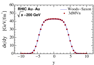
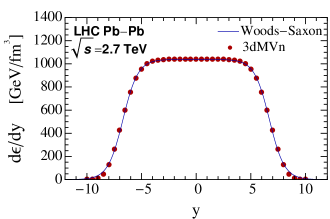
Figure 1: (Color online) $d\varepsilon/dy$ as a function of rapidity $y$ for central Au-Au collisions at RHIC (upper panel) and central Pb-Pb collisions at LHC (lower panel). $d\varepsilon/dy$ can also be taken as $\varepsilon(\eta_{\mathrm{s}})$ (see text). The shape of the energy density from 3dMVn is fitted well by a Woods-Saxon profile in both cases.

Now we turn to the discussion of finding $\varepsilon(\eta_{\mathrm{s}})$ from $d\varepsilon/dy$. Let us recall that

$$\frac{d\varepsilon}{dy}=\frac{dE}{dy\,\tau d\eta_{\mathrm{s}}d^{2}x_{\perp}},$$ (25)

where $\eta_{\mathrm{s}}$ is the space-time rapidity. The simple picture of the transverse structure in the cylindrical 3dMVn model ensures that the energy density is homogeneous as a function of $\mathbf{x}_{\perp}$ in the nuclear overlap zone (one can certainly go beyond this approximation, see Ref. Chen and Fries (2013)). Also, we have not solved the full non-boost invariant collision problem that would give us the $\eta_{\mathrm{s}}$ dependence. However, we will now postulate a relation between rapidity $y$ and space-time rapidity $\eta_{\mathrm{s}}$ that will allow us to estimate the dependence on $\eta_{\mathrm{s}}$. One reasonable ansatz follows from the Bjorken flow where we consider a Hubble-like velocity profile for the produced gluons, i.e., ${v_{z}=p_{z}/E\approx z/t}$ Bjorken (1983); Hirano and Nara (2004). This leads to ${y\approx\eta_{\mathrm{s}}}$, where ${\eta_{\mathrm{s}}\equiv\frac{1}{2}\ln\left[(t+z)/t-z\right]}$ and ${y\equiv\frac{1}{2}\ln\left[(E+p_{z})/E-p_{z}\right]}$ Therefore, our ansatz can be summarized as

$$\frac{dE}{dy\tau d\eta_{\mathrm{s}}d^{2}x_{\perp}}\approx\varepsilon(\eta_{\mathrm{s}})\delta(y-\eta_{\mathrm{s}}).$$ (26)

However, the $d\varepsilon/dy$ that we calculated in Eq. (23) did not have this correlation, rather it was flat in $\eta_{\mathrm{s}}$ for any fixed value of $y$ and must thus correspond to an averaged quantity

$$\frac{d\varepsilon}{dy}\Big{|}_{y\approx\eta_{\mathrm{s}}}\propto\int d\eta_{\mathrm{s}}\frac{dE}{dy\tau d\eta_{\mathrm{s}}d^{2}x_{\perp}}\,.$$ (27)

This leads to the relation

$$\varepsilon(\eta_{\mathrm{s}})\propto\frac{d\varepsilon}{dy}\Big{|}_{y\approx\eta_{\mathrm{s}}}.$$ (28)

Thus we infer that the momentum rapidity profile would coincide with the space-time rapidity profile. However, we will not attempt to find the proportionality constant between $\varepsilon(\eta_{\mathrm{s}})$ and $d\varepsilon/dy$. This result could be generalized by allowing additional smearing around the $y=\eta_{\mathrm{s}}$ relation.

The normalizations of our results depend only weakly on the correlation length $\lambda$, but they are sensitive to the choice of $\alpha_{\mathrm{s}}$, ${\Lambda_{\mathrm{UV}}\sim Q_{\mathrm{s}}}$, ${\langle m_{\mathrm{T}}\rangle}$, and the nuclear volume $V$. However, reasonable values for these parameters lead to a normalization of $\varepsilon(\eta_{\mathrm{s}})$ which is comparable to the typical initial conditions used in hydrodynamics simulations. Our main result here is the shape of the rapidity dependence of the initial energy density, which is much more stable against the variations of the parameters. Note that the uncertainty grows significantly at large rapidities $|\eta_{\mathrm{s}}|\approx|y|\approx y_{\mathrm{beam}}$. Our numerical calculations exhibit a plateau around mid-rapidity and a fall-off toward beam rapidity that is about three units of rapidity wide at both energies. The shape is fitted well by a Woods-Saxon profile

$$\varepsilon(\eta_{\mathrm{s}})=\frac{\varepsilon_{0}}{1+\exp\left[(|\eta_{\mathrm{s}}|-\eta_{\mathrm{flat}})/a\right]}\,.$$ (29)

The values of the Woods-Saxon parameters for RHIC and LHC are given in Table 1.

Our Woods-Saxon parametrization is somewhat different from the usual phenomenological parametrization of the initial energy density used by most groups employing (3+1)$D$ hydrodynamics, which consists of a perfectly flat plateau around mid-rapidity flanked by two half-Gaussian functions Hirano (2002); Schenke et al. (2010). It remains to be seen whether the differences between our calculated shape and the empirical assumptions in the literature can be resolved experimentally. However, our calculation makes quantitative predictions of the width of the plateau and the width of the fall-off towards the beam rapidity, albeit within the limitations of the approximations used.

Our results can be compared with the ones in Ref. Hirano and Nara (2004), which use different assumptions. In that reference the energy density is extracted from the number density, which in turn comes from a $k_{T}$-factorized ansatz involving UGDs. The $x$ dependence of those UGDs does not come directly from the three-dimensional structure of the nuclei but from phenomenological fits. While the result in Ref. Hirano and Nara (2004) might encode some quantum corrections that are not included in our work, it also uses a set of assumptions which go beyond the ones used here.

Table 1: The list of parameters for the Woods-Saxon parametrization of $d\varepsilon/dy\,[\mathrm{GeV/fm^{3}}]$ given in Eq. (29). Within the approximation of Eq. (28), this table can be seen as a list of parameters for $\varepsilon(\eta_{\mathrm{s}})$ as well. Although there is a large uncertainty in the parameter $\varepsilon_{0}$, the ratio of $\varepsilon_{0}$ for RHIC to LHC is in compliance with the ratio that can be calculated for the Stefan-Boltzmann law given the typical RHIC and LHC temperatures. While varying one of the parameters $\alpha_{\mathrm{s}}$, $\lambda$ and $\langle m_{\mathrm{T}}\rangle$, we keep the other two fixed to $\alpha_{\mathrm{s}}=0.4$, $\lambda=1.8\;\mathrm{fm}$ and $\langle m_{\mathrm{T}}\rangle=0.7\;\mathrm{GeV}$ for RHIC, and $\alpha_{\mathrm{s}}=0.4$, $\lambda=1.8\;\mathrm{fm}$ and $\langle m_{\mathrm{T}}\rangle=1.3\;\mathrm{GeV}$ for LHC.

			RHIC			LHC
		$\varepsilon_{0}$	$\eta_{\mathrm{flat}}$	$a$	$\varepsilon_{0}$	$\eta_{\mathrm{flat}}$	$a$
$\alpha_{\mathrm{s}}$	0.2	5.8	4.6	0.7
	0.3	19	4.6	0.7	477	6.7	0.7
	0.4	43	4.6	0.7	1091	6.7	0.7
	0.5	77	4.6	0.7	2024	6.7	0.7
$\lambda$	1.4	34	4.7	0.6	892	6.8	0.7
	1.6	39	4.7	0.6	995	6.8	0.7
	1.8	43	4.6	0.7	1091	6.7	0.7
	2.0	46	4.6	0.7	1180	6.6	0.7
	2.2	50	4.5	0.7	1264	6.6	0.7
$\langle m_{\mathrm{T}}\rangle$	0.5	84	4.9	0.7
	0.7	43	4.6	0.7
	0.9	26	4.4	0.7	2276	7.1	0.7
	1.1	17	4.2	0.7	1524	6.9	0.7
	1.3	12	4	0.7	1091	6.7	0.7
	1.5				819	6.6	0.7
	1.7				638	6.4	0.7

V Summary and Outlook

We have estimated the initial energy density per momentum space rapidity $d\varepsilon/dy$ as a function of $y$ at very small ${\tau\approx 0}$ in the three-dimensional, color neutral McLerran-Venugopalan model. We have further made an assumption about the correlation between the momentum space rapidity and space-time rapidity, which ultimately allowed us to determine the energy density as a function of $\eta_{\mathrm{s}}$. The initial energy density is an important input, poorly constrained thus far, for current hydrodynamic simulations of heavy-ion collisions. While hydrodynamics sets in at times somewhat later than $\tau\approx 0$, we argue that our results can nevertheless be useful as constraints. The normalization of the energy density depends strongly on some of the parameters, but we found that for reasonable values of these parameters the normalizations had the correct order of magnitude. Our main result is the shape of the energy density as a function of rapidity. We provided a parametrization of our result in terms of a Woods-Saxon function. Our result is complementary to others found in the literature.

Approaches that first calculate the number density of gluons have to make assumptions about how to relate the number of gluons to the energy density as well as the time at which this matching should be done. We have followed an approach that calculates the energy density $T^{00}$ directly at a time $\sim R/\gamma$.

It should be straightforward to work the rapidity profile we found here into the (3+1)$D$ hydrodynamics codes, also including fluctuations of the energy density in the transverse plane. It would also be interesting to consider fluctuations in the longitudinal direction, which are beyond the scope of this work.

References

- Adcox et al. (2005) K. Adcox et al. (PHENIX Collaboration), Nucl.Phys. A757, 184 (2005).
- Adams et al. (2005) J. Adams et al. (STAR Collaboration), Nucl.Phys. A757, 102 (2005).
- Muller et al. (2012) B. Muller, J. Schukraft, and B. Wyslouch, Ann.Rev.Nucl.Part.Sci. 62, 361 (2012).
- McLerran and Venugopalan (1994a) L. D. McLerran and R. Venugopalan, Phys.Rev. D49, 2233 (1994a).
- McLerran and Venugopalan (1994b) L. D. McLerran and R. Venugopalan, Phys.Rev. D49, 3352 (1994b).
- Kovchegov (1996) Y. V. Kovchegov, Phys.Rev. D54, 5463 (1996).
- Iancu and Venugopalan (2003) E. Iancu and R. Venugopalan, In *Hwa, R.C. (ed.) et al.: Quark Gluon Plasma* , 249 (2003), arXiv:hep-ph/0303204 [hep-ph] .
- Kovner et al. (1995a) A. Kovner, L. D. McLerran, and H. Weigert, Phys.Rev. D52, 6231 (1995a).
- Kovner et al. (1995b) A. Kovner, L. D. McLerran, and H. Weigert, Phys.Rev. D52, 3809 (1995b).
- Fries et al. (2006) R. Fries, J. Kapusta, and Y. Li, (2006), arXiv:nucl-th/0604054 [nucl-th] .
- Lappi and McLerran (2006) T. Lappi and L. McLerran, Nucl.Phys. A772, 200 (2006).
- Chen and Fries (2013) G. Chen and R. J. Fries, Phys.Lett. B723, 417 (2013).
- Song and Heinz (2009) H. Song and U. W. Heinz, J.Phys. G36, 064033 (2009).
- Fries and Nonaka (2011) R. Fries and C. Nonaka, Prog.Part.Nucl.Phys. 66, 607 (2011).
- Gale et al. (2013) C. Gale, S. Jeon, and B. Schenke, Int.J.Mod.Phys. A28, 1340011 (2013).
- Lappi (2006) T. Lappi, Phys.Lett. B643, 11 (2006).
- Schenke et al. (2012a) B. Schenke, P. Tribedy, and R. Venugopalan, Phys.Rev.Lett. 108, 252301 (2012a).
- Schenke et al. (2012b) B. Schenke, P. Tribedy, and R. Venugopalan, Phys.Rev. C86, 034908 (2012b).
- Lam and Mahlon (1999) C. Lam and G. Mahlon, Phys.Rev. D61, 014005 (1999).
- Lam and Mahlon (2000) C. Lam and G. Mahlon, Phys.Rev. D62, 114023 (2000).
- Ozonder (2013a) S. Ozonder, Phys. Rev. D 87, 045013 (2013a).
- Ozonder (2013b) S. Ozonder, Phys. Rev. D 87, 069902 (2013b), [erratum].
- Jimenez-Delgado and Reya (2009) P. Jimenez-Delgado and E. Reya, Phys.Rev. D80, 114011 (2009).
- Hirano and Nara (2004) T. Hirano and Y. Nara, Nucl.Phys. A743, 305 (2004).
- Krasnitz and Venugopalan (1999) A. Krasnitz and R. Venugopalan, Nucl.Phys. B557, 237 (1999).
- Makhlin (1996) A. Makhlin, (1996), arXiv:hep-ph/9608261 [hep-ph] .
- Fujii et al. (2009) H. Fujii, K. Fukushima, and Y. Hidaka, Phys.Rev. C79, 024909 (2009).
- Bjorken (1983) J. Bjorken, Phys.Rev. D27, 140 (1983).
- Hirano (2002) T. Hirano, Phys.Rev. C65, 011901 (2002).
- Schenke et al. (2010) B. Schenke, S. Jeon, and C. Gale, Phys.Rev. C82, 014903 (2010).