The RoboPol optical polarization survey of gamma-ray–loud blazars

Abstract

We present first results from RoboPol, a novel-design optical polarimeter operating at the Skinakas Observatory in Crete. The data, taken during the May – June 2013 commissioning of the instrument, constitute a single-epoch linear polarization survey of a sample of gamma-ray–loud blazars, defined according to unbiased and objective selection criteria, easily reproducible in simulations, as well as a comparison sample of, otherwise similar, gamma-ray–quiet blazars. As such, the results of this survey are appropriate for both phenomenological population studies and for tests of theoretical population models. We have measured polarization fractions as low as $0.015$ down to $R$ magnitude of 17 and as low as $0.035$ down to 18 magnitude. The hypothesis that the polarization fractions of gamma-ray–loud and gamma-ray–quiet blazars are drawn from the same distribution is rejected at the $3\sigma$ level. We therefore conclude that gamma-ray–loud and gamma-ray–quiet sources have different optical polarization properties. This is the first time this statistical difference is demonstrated in optical wavelengths. The polarization fraction distributions of both samples are well-described by exponential distributions with averages of $\langle p\rangle=6.4^{+0.9}_{-0.8}\times 10^{-2}$ for gamma-ray–loud blazars, and $\langle p\rangle=3.2^{+2.0}_{-1.1}\times 10^{-2}$ for gamma-ray–quiet blazars. The most probable value for the difference of the means is $3.4^{+1.5}_{-2.0}\times 10^{-2}$. The distribution of polarization angles is statistically consistent with being uniform.

1 Introduction

Blazars, which include BL Lac objects and Flat Spectrum Radio Quasars (FSRQs), represent the class of gamma-ray emitters with the largest fraction of members associated with known objects (Nolan et al., 2012). They are active galactic nuclei with their jets closely aligned to our line of sight (Blandford & Königl, 1979). Their emission is thus both beamed and boosted through relativistic effects, so that a large range of observed properties can result from even small variations in their physical conditions and orientation. As a result, the physics of jet launching and confinement, particle acceleration, emission, and variability, remain unclear, despite decades of intense theoretical and observational studies.

Blazars are broadband emitters exhibiting spectral energy distributions ranging from cm radio wavelengths to the highest gamma-ray energies (e.g. Giommi et al., 2012) with a characteristic “double-humped” appearance. While the mechanism of their high-energy (X-ray to gamma-ray) emission remains debatable, it is well established that lower-energy jet emission is due to synchrotron emission from relativistic electrons. Linear polarization is one property characteristic of the low-energy emission.

Polarization measurements of blazar synchrotron emission can be challenging, yet remarkably valuable. They probe parts of the radiating magnetised plasma where the magnetic field shows some degree of uniformity quantified by $\frac{B_{0}}{B}$ where $B_{0}$ is a homogeneous field and $B$ is the total field (e.g. Sazonov, 1972). The polarized radiation then carries information about the structure of the magnetic field in the location of the emission (strength, topology and uniformity). Temporal changes in the degree and direction of polarization can help us pinpoint the location of the emitting region and the spatiotemporal evolution of flaring events within the jet.

Of particular interest are rotations of the polarization angle in optical wavelengths during gamma-ray flares, instances of which have been observed through polarimetric observations concurrent with monitoring at GeV and TeV energies, with Fermi-LAT (Atwood et al., 2009) and MAGIC (Baixeras et al., 2004) respectively (e.g., Abdo et al., 2010; Marscher et al., 2008). If such rotations were proven to be associated with the outbursting events of the gamma-ray emission, then the optopolarimetric evolution of the flare could be used to extract information about the location and evolution of the gamma-ray emission region.

Such events have stimulated intense interest in the polarimetric monitoring of gamma-ray blazars (Hagen-Thorn et al., 2006; Smith et al., 2009; Ikejiri et al., 2011, e.g.,). These efforts have been focusing more on “hand-picked” sources and less on statistically well-defined samples aiming at maximising the chance of correlating events. Consequently, although they have resulted in the collection of invaluable optopolarimetric datasets for a significant number of blazars, they are not designed for rigorous statistical studies of the blazar population; the most obvious one being the investigation of whether the observed events are indeed statistically correlated with gamma-ray flares, or are the result of chance coincidence. The RoboPol program has been designed to bridge this gap.

The purpose of this paper is two-fold. Firstly, we aim to present the results of a survey that RoboPol conducted in June 2013, which is the first single-epoch optopolarimetric survey of an unbiased sample of gamma-ray–loud blazars. As such, it is appropriate for statistical phenomenological population studies and for testing blazar population models. Secondly, we wish to alert the community to our optopolarimetric monitoring program and to encourage complementary observations during the Skinakas winter shutdown of December – March.

After a brief introduction to the RoboPol monitoring program in Section 2, the selection criteria for the June 2013 survey sample and the July – November 2013 monitoring sample are reviewed in Section 3. The results from the June 2013 survey are presented in Section 4, where the optical polarization properties of the survey sample and possible differences between gamma-ray–loud and gamma-ray–quiet blazars are also discussed. We summarise our findings in Section 5.

2 The RoboPol optopolarimetric monitoring program

The RoboPol program has been designed with two guiding principles in mind:

1. to provide datasets ideally suited for rigorous statistical studies;

2. to maximise the potential for the detection of polarization rotation events.

To satisfy the former requirement, we have selected a large sample of blazars on the basis of strict, bias-free, objective criteria, which are discussed later in this paper. To satisfy the latter, we have secured a considerable amount of evenly allocated telescope time; we have constructed a novel, specially designed polarimeter – the RoboPol instrument – (A. N. Ramaprakash et al. , in preparation, hereafter “instrument” paper); and we have developed a system of automated telescope operation including data reduction that allows the implementation of dynamical scheduling (King et al. 2013, hereafter “pipeline” paper). The long-term observing strategy of the RoboPol program is the monitoring of $\sim$ 100 target (gamma-ray–loud) sources and an additional $\sim$15 control (gamma-ray–quiet) sources with a duty cycle of about 3 nights for non-active sources and several times a night for sources in an active state.

2.1 The RoboPol instrument

The RoboPol instrument (described in the “instrument” paper) is a novel-design 4-channel photopolarimeter. It has no moving parts, other than a filter wheel, and simultaneously measures both linear fractional Stokes parameters $q=Q/I$ and $u=U/I$. This design bypasses the need for multiple exposures with different half-wave plate positions, thus avoiding unmeasurable errors caused by sky changes between measurements and imperfect alignment of rotating optical elements. The instrument has a $13^{\prime}\times 13^{\prime}$ field of view, enabling relative photometry using standard catalog sources and the rapid polarimetric mapping of large sky areas. It is equipped with standard Johnson-Cousins $R$- and $I$-band band filters from Custom Scientific. The data presented in this paper are taken with the $R$-band filter. RoboPol is mounted on the 1.3-m, f/7.7 Ritchey–Cretien telescope at Skinakas Observatory (1750 m, $23^{\circ}53^{\prime}57^{\prime\prime}′$E, $35^{\circ}12^{\prime}43^{\prime\prime}$N, Papamastorakis, 2007) in Crete, Greece. It was commissioned in May 2013.

Table 1: Selection criteria for the gamma-ray–loud and the control sample. A summarising chart is shown in Fig. 1.

Property	Allowed range for the June survey	Allowed range for the 2013 monitoring
Gamma-ray–loud sample
2FGL $F\left(>100\right)$ MeV	$>2\times 10^{-8}{\rm\,cm^{-2}\,s^{-1}}$	$>2\times 10^{-8}{\rm\,cm^{-2}\,s^{-1}}$
2FGL source class	agu, bzb, or bzq	agu, bzb, or bzq
Galactic latitude $|b|$	$>10^{\circ}$	$>10^{\circ}$
Elevation (Elv) constraints1	$\mathrm{Elv}\geq 30^{\circ}$ for at least 30 min in June	$\mathrm{Elv_{max}}\geq 40^{\circ}$ for at least 120 consecutive days in the window June – November including June
$R$ magnitude	$\leq 18^{2}$	$\leq 17.5^{3}$
Control sample
CGRaBS/15 GHz OVRO monitoring	included	included
2FGL	not included	not included
Elevation constraints1	None	$\mathrm{Elv_{max}}\geq 40^{\circ}$ constantly in the window mid-April – mid-November
$R$ magnitude	$\leq 18$	$\leq 17.5^{2}$
OVRO 15 GHz mean flux density	N/A	$\geq 0.060$ Jy
OVRO 15 GHz intrinsic modulation index, $m$	$\geq 0.02$	$\geq 0.05$
Declination	$\geq 54.8^{\circ}$ (circumpolar)	N/A

¹Refers to elevation during Skinakas dark hours

²Archival value

³Average value between archival value and measured during preliminary RoboPol Skinakas observations in June 2012 (when applicable)

2.2 The first RoboPol observing season

In June 2013 RoboPol performed an optopolarimetric survey of a sample of gamma-ray–loud blazars, results from which are presented in this paper. Until November 2013, it was regularly monitoring (with a cadence of once every few days) an extended sample of blazars, described in Section 3. These sources were monitored until the end of the observing season at Skinakas (November 2013). The results of this first-season monitoring will be discussed in an upcoming publication.

2.3 Multi-band monitoring of the RoboPol sources

All of our sources (including the control sample) are monitored twice a week at 15 GHz by the OVRO 40-m telescope blazar monitoring program (Richards et al., 2011). 28 of them are also monitored at 30 GHz by the Toruń 32-m telescope (e.g. Browne et al., 2000; Peel et al., 2011). Additionally, our sample includes most sources monitored by the F-GAMMA program (Fuhrmann et al., 2007; Angelakis et al., 2010) that are visible from Skinakas; for these sources, the F-GAMMA program takes multi-band radio data (total power, linear and circular polarization) approximately once every 1.3 months. By design, Fermi-LAT in its sky-scanning mode is continuously providing gamma-ray data for all of our gamma-ray–loud sources. In this way, our sample has excellent multi-band coverage. These multiwavelength data will be used in the future to correlate the behaviour of our sample in optical flux and polarization with the properties and variations in other wavebands.

3 Sample selection criteria

3.1 Parent Sample

We construct a gamma-ray flux-limited “parent sample” of gamma-ray–loud blazars from the second Fermi-LAT source catalog (Nolan et al., 2012) using sources tagged as BL Lac (bzb), FSRQ (bzq), or active galaxy of uncertain type (agu). The parent sample is created the following way:

1. for each source, we add up Fermi-LAT fluxes above 100 MeV to obtain the integrated photon flux $F\left(>100\mathrm{\,MeV}\right)$,

2. we exclude sources with $F\left(>100{\rm\,MeV}\right)$ less than or equal to $2\times 10^{-8}$ cm^-2 s^-1, and

3. we exclude sources with galactic latitude $|b|\leq 10^{\circ}$.

This leaves us with 557 sources in the parent sample. We have verified that the sample is truly photon-flux-limited since there is no sensitivity dependence on spectral index or galactic latitude with these cuts. Of these 557 sources, 421 are ever observable from Skinakas: they have at least one night with airmass less than 2, (or, equivalently, elevation higher than $30^{\circ}$), for at least one hour, within the dark hours of the May – November observing window. Archival optical magnitudes were obtained for all 557 sources in the parent sample mostly in the $R$-band using the BZCAT (Massaro et al., 2009), CGRaBS (Healey et al., 2008a), LQAC 2 (Souchay et al., 2011) and GSC 2.3.2 (Lasker et al., 2008) catalogs .

3.2 June 2013 Survey Sample

The June 2013 survey sample was constructed of parent sample sources with a recorded archival $R$ magnitude less or equal to 18 ($R\leq 18$) which were visible from Skinakas during dark hours in the month of June 2013 for at least 30 min at airmass less than 2. The selection criteria for the candidate sources in this sample are summarised in Table 1. This selection resulted in 142 sources potentially observable in the month of June which constitute a statistically complete sample. The sources were observed according to a scheduling algorithm designed to maximise the number of sources that could be observed in a given time window based on rise and set times, location of sources on the sky, and resulting slewing time of the telescope. At the end of the survey, 133 of these sources had been observed. Because the scheduling algorithm was independent of intrinsic source properties, the resulting set of 133 observed sources is an unbiased subsample of the statistically complete sample of the 142 sources (summary in Fig. 1). The completeness of the sample is $93\,\%$ for sources brighter than 16 magnitude, $95\,\%$ ($81/85$) for sources brighter than 17 magnitude, and $94\,\%$ ($133/142$) for sources brighter than 18 magnitude.

To identify sources suitable for inclusion in the “control” sample, a number of non-2FGL CGRaBS (Candidate Gamma-Ray Blazar Survey, Healey et al., 2008a) blazars were also observed during the June survey. CGRaBS was a catalog of likely gamma-ray–loud sources selected to have similar radio and X-ray properties with then known gamma-ray–loud blazars. However, because Fermi has a much improved sensitivity at higher energies than its predecessors, Fermi-detected blazars include many sources absent from CGRaBS, with harder gamma-ray–spectra than CGRaBS sources, especially at lower gamma-ray fluxes. To ensure that non-CGRaBS sources among our gamma-ray–loud sample do not affect our conclusions when populations of gamma-ray–loud and gamma-ray–quiet blazars are found to have significantly different properties, in such cases we will also be performing comparisons between our “control” sample and that fraction of our gamma-ray–loud sample that is also included in CGRaBS.

Candidate sources for these observations were selected according to the criteria listed in table 1. There, the radio variability amplitude is quantified through the intrinsic modulation index $m$ as defined by Richards et al. (2011), which measures the flux density standard deviation in units of the mean flux at the source. For the sources discussed in Section 4, $m$ is reported in table 3. The criteria of table 1 result in a statistically complete sample of 25 in principle observable, circumpolar, gamma-ray–quiet sources. Of these, 17 sources were observed (71 %), in order of decreasing polar distance, until the end of our June survey. Since the polar distance criterion is independent of source properties, the resulting gamma-ray–quiet sources is again an unbiased subsample of the statistically complete sample of 25 sources. This unbiased subsample is 86 % ($6/7$) complete for sources with $R$-mag $\leq 16$, 92 % ($11/12$) for sources with $R$-mag $\leq 17$ and of course 71 % ($17/24$) for sources with $R$-mag $\leq 18$.

Our gamma-ray–loud sources are (by construction of CGRaBS) similar in radio and X-ray flux, and radio spectra. Their R-Magnitudes span a similar range and have a similar distribution as can be seen a posteriori (see Fig. 3). The radio modulation indices have been shown to be systematically higher for gamma-ray–loud sources in general Richards et al. (2011); to counter this effect, we select, among the gamma-ray–quiet candidates, only sources with statistically significant radio variability, as quantified by the modulation index (see table 1). The gamma-ray–loud sample has fractionally more BL Lacs (about 50%) than the gamma-ray–quiet control sample (about 10%), which is expected when comparing gamma-ray–loud with gamma-ray–quiet samples, but which should, however, be taken into account when interpreting our results.

The June 2013 survey results are discussed in Section 4.

3.3 Monitoring Sample

The data collected during the survey phase were used for the construction of the 2013 observing season monitoring sample which was observed from July 2013 until the end of the 2013 observing season, with an approximate average cadence of once every 3 days. It consists of three distinct groups.

1. An unbiased subsample of a statistically complete sample of gamma-ray–loud blazars. Starting from the “parent sample” and applying the selection criteria summarised in Table 1, we obtain a statistically complete sample of 59 sources. Application of field-quality cuts (based on data from the June survey) and location-on-the-sky criteria that optimise continuous observability results in an unbiased subsample of 51 sources.

2. An unbiased subsample of a statistically complete sample of gamma-ray–quiet blazars. Starting from the CGRaBS, excluding sources in the 2FGL, and applying the selection criteria summarised in Table 1 results in a statistically complete sample of 22 sources. Our “control sample” is then an unbiased subsample of 10 blazars, selected from this complete sample of gamma-ray–quiet blazars with field-quality and location-on-the-sky criteria.

3. 24 additional “high interest” sources, that did not otherwise make it to the sample list.

These observations will later allow the characterisation of each source’s typical behaviour (i.e. average optical flux and degree of polarization, rate of change of polarization angle, flux and polarization degree variability characteristics). This information will be further used to:

1. improve the optical polarization parameters estimates for future polarization population studies,

2. develop a dynamical scheduling algorithm, aiming at self-triggering higher cadence observing for blazars displaying interesting polarization angle rotation events, for the 2014 observing season,

3. improve the definition of our 2014 monitoring sample using a contemporary average, rather than archival single-epoch, optical flux criterion along with some estimate of the source variability characteristics in total intensity and in polarized emission.

For the June survey control sample sources, circumpolar sources were selected so that gamma-ray–quiet source observations could be taken at any time and the gamma-ray–loud sources could be prioritized. In contrast, the gamma-ray–quiet sources for the monitoring sample were selected in order of increasing declination, to avoid as much as possible the northernmost sources which suffer from interference in observations by strong northern winds at times throughout the observing season at Skinakas.

The steps followed for the selection of the June survey sample and the first season monitoring one are summarised schematically in Fig. 1. The complete sample of our monitored sources is available at robopol.org.

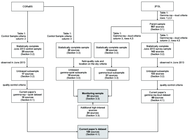
Figure 1: Flow chart indicating the steps for the selection of (a) left-hand half: the gamma-ray–quiet “control” sample and (b) right-hand half: the gamma-ray–loud sample, separately for the monitoring program of 2013 and the current paper’s study.

The 2nd Fermi gamma-ray catalog, from which the parent gamma-ray-loud sample is drawn, represents a “from-scratch” all-sky survey in $\geq 100$ MeV gamma-rays, so the limit in gamma-ray flux should in principle result in a clean, flux-limited sample. One possible source of bias however is the process of characterisation of a source as a “blazar”, in which case other catalogs of blazars (principally from radio surveys) are used for the identification and classification of sources. Given that 575 of the 1873 Fermi catalog sources are unassociated, that bias may in fact be non-trivial: we don’t know how many of the unassociated sources are blazars, and we cannot a priori be certain that the properties of any blazars among the unassociated sources are similar to those of confidently associated blazars. Unassociated sources are not however uniformly distributed among fluxes and Galactic latitudes. Brighter sources, sources in high Galactic latitudes, and sources with hard spectra tend to have smaller positional error circles and are more easily associated with low-energy counterparts (because of more photons available for localization, lower background, and better single-photon localization at higher energies, respectively). The first of these two factors lower the fraction of unassociated sources among the 2FGL sources that satisfy our Galactic latitude and gamma-ray–flux cuts, from $\sim 30\%$ to $\sim 20\%.$ The effect of possible biases due to the presence of unassociated sources in 2FGL can be further assessed, as part of theoretical population studies, under any particular assumption regarding the nature of these sources, as well as if, at some point in the future, a large fraction of these sources become confidently associated with low-energy counterparts.

Any other minor biases entering through our choices of limits in gamma-ray flux and $R$ magnitude can be accounted for in theoretical population studies given the cuts themselves, the uncertainty distribution in the measured quantities (which can be found in the literature), and some knowledge of the variability of these sources (obtainable from Fermi data in gamma rays, and, at the most basic level, from comparing historical magnitudes with magnitudes from this work in the R-band).

4 Results of June 2013 Survey

4.1 Observations

The June survey observations took place between June 1st and June 26th. During that period, we conducted RoboPol observations, weather permitting, for 21 nights. Of those, 14 nights had usable dark hours. The most prohibiting factors have been wind, humidity and dust, restricting the weather efficiency to 67 %, unusually low based on historical Skinakas weather data. During this period, a substantial amount of observing time was spent on system commissioning activities. In the regular monitoring mode of operations a much higher efficiency is expected.

During the survey phase a total of 135 gamma-ray–loud targets (133 of them comprising the unbiased subsample of the 142-source sample and 2 test targets), 17 potential control-sample sources, and 10 polarization standards, used for calibration purposes, were observed. For the majority of the sources, a default exposure time of $15-17.5$ min divided into 3 exposures was used to achieve a polarization sensitivity of ${\rm SNR}_{p}=10:1$ for a 17 mag source with polarization fraction of 0.03, based on the instrument sensitivity model. Shorter total exposures were used for very bright sources and standard stars, and their duration was estimated on-the-fly. Typically we observed 2 different polarimetric standards every night to confirm the stability of the instrument (see “pipeline” paper).

In summary, we observed 133 + 17 blazars belonging to the unbiased subsamples of the gamma-ray–loud and gamma-ray–quiet complete samples respectively. Of these sources, 89 gamma-ray–loud and 15 gamma-ray–quiet sources passed a series of unbiased, source-property–independent quality-control criteria to ensure accurate polarization measurements (see Fig. 1).

The RoboPol results for these 89 + 15 sources are shown in Table 2. These results include: the $R$-magnitude, calibrated with two different standards [the Palomar Transient Factory (PTF) $R$-band catalog (Ofek et al., 2012, whenever available) or the USNO-B catalog (Monet et al., 2003)]; the polarization fraction, $p=\sqrt{u^{2}+q^{2}}$; and the polarization angle, $\chi=\frac{1}{2}\arctan\left(\frac{u}{q}\right),$ measured from the celestial north counter-clockwise. In that table target sources are identified by the prefix “RBPL” in their RoboPol identifying name. Additional archival information for these sources are given in Table 3, available as online as supplementary material.

The images were processed using the data reduction pipeline described in the “pipeline” paper. The pipeline performs aperture photometry, calibrates the measured counts according to an empirical instrument model, calculates the linear polarization fraction $p$ and angle $\chi$, and performs relative photometry using reference sources in the frame to obtain the $R$-band magnitude. Entries in table 2 with no photometry information are sources for which PTF data do not exist and the USNO-B data were not of sufficient quality for relative photometry. Polarimetry, for which only the relative photon counts in the four spots are necessary, can still of course be performed without any problem in these cases. The photometry error bars are dominated by uncertainties in our field standards, while the polarization fraction and angle errors are photon-count dominated. For the few cases where multiple observations of a source were obtained in June, weighted averaging of the $q$ and $u$ has been performed. The quoted uncertainty follows from formal error propagation assuming that $q$ and $u$ follow normal distributions and that the polarization has not changed significantly between measurements.

4.2 Debiasing

The $p$ values and uncertainties $\sigma_{p}$ shown in Table 2 are the raw values as produced by the pipeline, without any debiasing applied to them, and without computing upper limits at specific confidence levels for low $p/\sigma_{p}$ ratios. Debiasing is appropriate for low signal-to-noise measurements of $p$ because measurements of linear polarization are always positive and for any true polarization degree $p_{0}$ we will, on average, measure $p>p_{0}$. Vaillancourt (2006) gives approximations for the maximum-likelihood estimator of $p_{0}$ at various $p/\sigma_{p}$ levels, and describes how to calculate appropriate upper limits for specific confidence levels. He finds that the maximum-likelihood estimator is well approximated by

$$\hat{p}=\left\{\begin{array}[]{lll}0&&\mbox{for $p/\sigma_{p}<\sqrt{2}$}\\ \sqrt{p^{2}-\sigma_{p}^{2}}&&\mbox{for $p/\sigma_{p}\gtrsim 3$}\end{array}\right.$$ (1)

For $p/\sigma_{p}\gtrsim 3$ the assumption of a normal distribution for $p-$measurements is also acceptable (and it is a good assumption for $p/\sigma_{p}\gtrsim 4$). Debiasing is not necessary for polarization angles $\chi$, as the most probable measured value is the true $\chi$ and as a result the pipeline output is an unbiased $\chi$ estimator.

Whenever in the text debiased $p$ values are mentioned, we are referring to a correction using $p_{\rm debiased}\approx\sqrt{p^{2}-\sigma_{p}^{2}}$ down to $p/\sigma_{p}=\sqrt{2}$ and 0 for lower signal-to-noise ratios (a choice frequently used in the literature), despite the fact that below $p/\sigma_{p}\sim 3$ this recipe deviates from the maximum-likelihood estimator. When a good estimate of the uncertainty is also necessary (i.e. in our likelihood analyses), we only use measurements with $p/\sigma_{p}>3$, for which not only the debiasing recipe we use is close to the maximum-likelihood estimator, but also the uncertainty calculated by the pipeline $\sigma_{p}$ is a reasonable approximation to the $68\%$ uncertainty in the value of $p$.

4.3 Polarization properties of gamma-ray–loud vs gamma-ray–quiet blazars

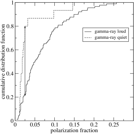
Figure 2: Cumulative distribution functions of raw $p$ values for all 89 gamma-ray–loud blazars (solid line) and 15 gamma-ray–quiet blazars (dashed line) with observations in June 2013 that passed all our quality cuts. The maximum difference between the two ($=0.6$) is shown with the double arrow. The hypothesis that the two samples are drawn from the same distribution is rejected at the $4\times 10^{-4}$ level ($3.5\sigma$).

As the unbiased nature of our samples allows us to address issues related to the blazar population, we wish to ask the question: are the measured polarization fractions of gamma-ray–loud and gamma-ray–quiet blazars consistent with having been drawn from the same distribution?

Because our observing strategy and data processing pipeline is uniform across sources, if the intrinsic polarization fractions of gamma-ray–loud and gamma-ray–quiet sources were indeed drawn from the same distribution, then the resulting observed distributions of $p$ would also be consistent with being the same. Each of them might not be consistent with the intrinsic $p$ distribution of the blazar population, because of biasing, and because at low $p/\sigma_{p}$ values what is being recorded is in general more noise than information; however, biasing and noise would affect data points in both populations in the same way and at the same frequency, and the resulting observed distributions, no matter how distorted, would be the same for the two subpopulations.

For this reason, we compare the observed raw $p-$values (as they come out of the pipeline) of the two samples of 89 gamma-ray–loud sources and 15 gamma-ray–quiet sources. Figure 2 shows the cumulative distribution functions (CDFs) of raw $p$ values for the gamma-ray–loud blazars (solid line) and the gamma-ray–quiet blazars (dashed line). The maximum difference between the two CDFs (indicated with the double arrow) is $0.58$, and a two-sample Kolmogorov-Smirnov test rejects the hypothesis that the two samples are drawn from the same distribution at the $4\times 10^{-4}$ level ($3.5\sigma$). The observed raw $p-$distributions are therefore inconsistent with being identical, and, as a result, the underlying distributions of intrinsic $p$ cannot be identical either.

As discussed in §3.2, while the gamma-ray–quiet sample is a pure subsample of CGRaBS, the gamma-ray–loud sample contains many (47) non-CGRaBS sources, which, in practice, means that the fraction of BL Lac objects (bzb) is much higher. To test whether this is the source of the discrepancy, we have repeated the same test between the 42 CGRaBS sources in our gamma-ray–loud sample, and the 15 sources in our gamma-ray–quiet sample. The maximum difference between the two CDFs in this case is $0.54$, so the hypothesis that the two distributions are identical is again rejected at the $3\times 10^{-3}$ level ($3\sigma$).

We conclude that the optical polarization properties of gamma-ray–loud and gamma-ray–quiet sources are different.

4.4 Polarization fraction vs $R$ magnitude

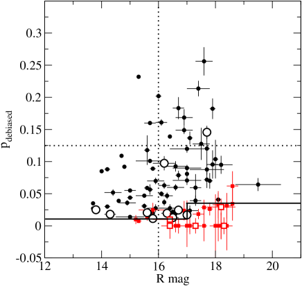
Figure 3: Debiased polarization fraction versus $R$ magnitude. Above the solid line, we assume that we can measure polarization independently of source brightness (for details see Sect. 4). Black circles correspond to measurements with $p/\sigma_{p}\geq 3$, and red squares to measurements with $p/\sigma_{p}<3$. Filled symbols correspond to gamma-ray–loud sources and open symbols to gamma-ray–quiet sources.

We next turn our attention to the behaviour of the polarization fraction with $R$ magnitude. In Fig. 3 we plot the debiased value of the polarization fraction as a function of the measured $R$ magnitude for each source. Sources for which $p/\sigma_{p}<3$ are shown with red colour. There are two noteworthy pictures in this plot: the clustering of low signal-to-noise ratio measurements in the lower-right corner of the plot, and the scarcity of observations in the upper-left part of the plot.

The first effect is expected, as low polarization fractions are harder to measure for fainter sources with fixed time integration. This is a characteristic of the June survey rather than the RoboPol program in general: in monitoring mode, RoboPol scheduling features adaptive integration time to achieve a uniform signal-to-noise ratio down to a fixed polarization value for any source brightness. For source brightness higher than magnitude of 17 we have measured polarization fractions down to $1.5\times 10^{-2}$: most measurements at that level have $p/\sigma_{p}\geq 3$. For source brightness lower than magnitude of 17 the same is true for polarization fractions down to $3.5\times 10^{-2}$. These limits are shown with the thick solid line in Fig. 3, and they are further discussed in Section 4.5 in the context of our likelihood analysis to determine the most likely intrinsic distributions of polarization fractions for gamma-ray–loud and gamma-ray–quiet sources.

The second effect – the lack of data points for $R$ magnitudes lower than 16 and polarization fractions higher than $1.25\times 10^{-1}$ as indicated by the dotted lines – may be astrophysical in origin: in sources where unpolarized light from the host galaxy is a significant contribution to the overall flux, the polarization fraction should be on average lower. This contribution also tends to make these sources on average brighter. We will return to a quantitative evaluation and analysis of this effect when we present data from our first season of monitoring, using both data from the literature as well as our own variability information to constrain the possible contribution from the host for as many of our sources as possible.

4.5 Intrinsic distributions of polarization fraction

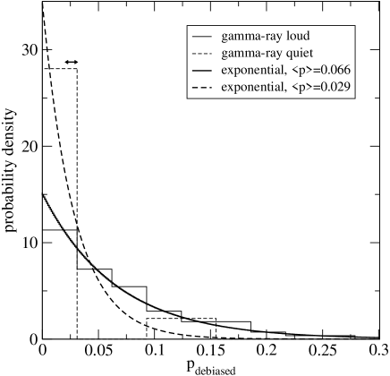
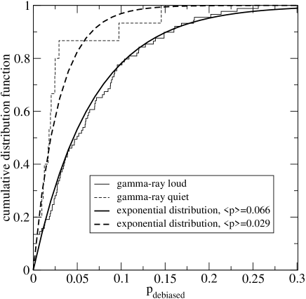
Figure 4: Histogram (upper panel) and cumulative distribution function (lower panel) of debiased $p$ values for all 89 gamma-ray–loud (thin solid lines) and 15 gamma-ray–quiet (dashed lines) blazars that pass quality cuts. The typical measurement uncertainty is shown in the upper panel with the arrow; the uncertainty spread is $\sim 10\%$ of that value. Thick solid and dashed lines correspond to the PDF and CDF of exponential distributions with average equal to the sample average of each population.

In Section 4.3 we showed that the intrinsic distributions of polarization fraction of gamma-ray–quiet and gamma-ray–loud blazars must be different; however, that analysis did not specify what these individual intrinsic distributions might be. We address this issue in this section. Our approach consists of two steps. First, we will determine what the overall shape of the distributions looks like, and we will thus select a family of probability distribution functions that can best describe the intrinsic probability distribution of polarization fraction in blazars. Next, we will use a likelihood analysis to produce best estimates and confidence limits on the parameters of these distributions for each subpopulation.

4.5.1 Selection of Family of Distributions

In order to determine the family of distributions most appropriate to describe the polarization fraction of the blazar population we plot, in the upper panel of Fig. 4, a histogram – normalised so that it represents a probability density – of all the debiased $p$ values in the gamma-ray–loud and gamma-ray–quiet samples, independently of their $p/\sigma_{p}$ ratio (89 and 15 sources, respectively). It appears that these histograms resemble exponential distributions. Indeed, in the upper panel of Fig. 4, we also over-plot the exponential distributions with mean equal to the sample average of $p$ for each sample, and we see that there is good agreement in both cases. To verify that our choice of binning does not affect the appearance of these distributions, we also plot, in the lower panel of Fig. 4, the CDF of each sample, as well as the CDFs corresponding to each of the model PDFs in the upper panel. The agreement is again excellent. We conclude that the PDFs of the polarization fraction of gamma-ray–quiet and gamma-ray–loud blazar subpopulations can be well described by exponential distributions.

4.5.2 Determination of Distribution Parameters

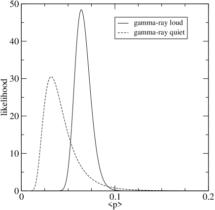
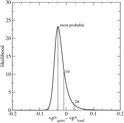
Figure 5: Likelihood of $\left<p\right>$ for each population (upper panel) and of the difference of $\left<p\right>$ between the two populations (lower panel). The most-probable values differ by about a factor of 2.

In this section, we seek to determine the best estimate values and associated confidence intervals for the parameters of the intrinsic PDFs of polarization fraction for our two blazar subpopulations. All values of $p$ used in this section are debiased as described in Section 4.2. Based on the results of our previous discussion, we will assume that the probability distribution of $p$ in a sample of blazars can be described as

$$P(p)dp=\frac{1}{\langle p\rangle}\exp\left(-\frac{p}{\langle p\rangle}\right)dp\,.$$ (2)

In order to be formally correct, there should be a factor of $1-{\rm e}^{-1/\langle p\rangle}$ in the denominator of Equation 2 to correct for the fact that $p$ is defined in the $[0,1]$ rather than the $[0,\infty)$ interval; the correction is however small for the values of $\langle p\rangle$ that are of interest here. The mean, $\langle p\rangle$, is the single parameter of this family of distributions, and it is the quantity that we seek to estimate from our data for each subsample.

In the population studies that follow, we will include only sources with $p/\sigma_{p}\geq 3$. However, in order to avoid biasing our statistics by this choice, we apply sharp cuts in $p-$space that exclude most, if not all, of our low $p/\sigma_{p}$ measurements; these cuts can then be explicitly corrected for in our analysis (which will assume that sources below a certain $p$ value do exist, in numbers predicted by the exponential distribution, but cannot be measured). These selection criteria are visualised by the thick solid line in Fig. 3.

We thus split each population into two sub-samples, along the (measured) $R$-mag 17 line, and, for each population, we consider each subsample to be a distinct “experiment” with a different data cut ($1.5\times 10^{-2}$ for bright sources and $3.5\times 10^{-2}$ for faint sources). We then use a likelihood analysis to estimate the maximum-likelihood value of the average $\langle p\rangle$ for each population, in a fashion similar to the one implemented for population studies in Richards et al. (2011). The sources for which no photometry information is available are considered part of our second experiment and the stricter cut is applied to them. In all our calculations below we use debiased values of $p$.

The likelihood of a single observation of a polarization fraction $p_{i}$ of (approximately) Gaussian uncertainty $\sigma_{i}$ drawn from the distribution of Eq. (2) with mean $\langle p\rangle$ can be approximated by

$$\ell_{i} = \!\!\!\!\!\!\int_{p=0}^{\infty}dp\frac{1}{\langle p\rangle}\exp\left(-\frac{p}{\langle p\rangle}\right)\frac{\exp\left[-\frac{(p-p_{i})^{2}}{2\sigma_{i}^{2}}\right]}{\sigma_{i}\sqrt{2\pi}}$$

$$= \frac{1}{2\langle p\rangle}\exp\left[-\left(\frac{p_{i}}{\langle p\rangle}-\frac{\sigma_{i}^{2}}{2\langle p\rangle^{2}}\right)\right]\times$$

$$\left[1+{\rm erf}\left(\frac{p_{i}}{\sigma_{i}\sqrt{2}}-\frac{\sigma_{i}}{\sqrt{2}\langle p\rangle}\right)\right].$$

Extending the upper limit of integration to $\infty$ instead of 1 simplifies the mathematics while introducing no appreciable change in our results, as the exponential distribution approaches 0 fast at $p<1$ for the data at hand. This can be directly seen in Fig. 4.

In order to implement data cuts restricting $p_{i}$ to be smaller than some limiting value $p_{l}$, the likelihood of a single observation $p_{i}$ will be given by Eq. 4.5.2 multiplied by a Heaviside step function, and re-normalised so that the likelihood $\ell_{i,\rm cuts}$ to obtain any value of $p_{i}$ above $p_{l}$ is 1:

$$\ell_{i,\rm cuts}\left(p_{l}\right)=\frac{H(p_{i}-p_{l})\ell_{i}}{\int_{p_{i}=p_{l}}^{1}dp_{i}\ell_{i}}\,.$$ (4)

This re-normalisation “informs” the likelihood that the reason why no observations of $p_{i}<p_{l}$ are made is not because such objects are not found in nature, but rather because we have excluded them “by hand.” We are, in other words, only sampling the $p>p_{l}$ tail of an exponential distribution of mean $\langle p\rangle$. The likelihood of $N$ observations of this type is

$$\mathcal{L}(\langle p\rangle)=\prod_{i=1}^{N}\ell_{i,\rm cuts}\left(p_{l}\right)\,,$$ (5)

and the combination of two experiments with distinct data cuts, described above, will have a likelihood equal to

$$\mathcal{L}(\langle p\rangle)=\prod_{i=1}^{N_{l}}\ell_{i,\rm cuts}\left(p_{l}\right)\prod_{j=1}^{N_{u}}\ell_{j,\rm cuts}\left(p_{u}\right)\,,$$ (6)

where $N_{l}$ (equal to 42 for the gamma-ray–loud sources and 6 for the gamma-ray–quiet sources) is the number of $p/\sigma_{p}>3$ objects with $R$-mag $<17$ surviving the $p_{l}=0.015$ cut, and $N_{u}$ (equal to 21 for the gamma-ray–loud sources and 1 for the gamma-ray–quiet sources) is the number of $p/\sigma_{p}>3$ objects with $R$-mag $>17$ or no photometry information surviving the $p_{u}=0.035$ cut. Maximising Eq. (6) we obtain the maximum-likelihood value of $\langle p\rangle$. Statistical uncertainties on this value can also be obtained in a straight-forward way, as Eq. (6), assuming a flat prior on $\langle p\rangle$, gives the probability density of the mean polarization fraction $\langle p\rangle$ of the population under study.

The upper panel of Fig. 5 shows the likelihood of $\langle p\rangle$ for the gamma-ray–loud (solid line) and gamma-ray–quiet (dashed line) populations. The maximum-likelihood estimate of $\langle p\rangle$ with its 68% confidence intervals is $6.4^{+0.9}_{-0.8}\times 10^{-2}$ for gamma-ray–loud blazars and $3.2^{+2.0}_{-1.1}\times 10^{-2}$ for gamma-ray–quiet blazars. The maximum-likelihood values of $\langle p\rangle$ differ by more than a factor of 2, consistent with our earlier finding that the two populations have different polarization fraction PDFs. However, because of the small number of gamma-ray–quiet sources surviving the strict signal-to-noise cuts we have imposed in this section (only 7 objects), the gamma-ray–quiet $\langle p\rangle$ cannot be pinpointed with enough accuracy and its corresponding likelihood exhibits a long tail towards high values. For this reason, the probability distribution of the difference between the $\langle p\rangle$ of the two populations, which is quantified by the cross-correlation of the two likelihoods, has a peak, at a difference of $3.1\times 10^{-2}$, which is less than 2$\sigma$ from zero. This result is shown in the lower panel of Fig. 5.

The accuracy with which the gamma-ray–quiet $\langle p\rangle$ is estimated can be improved in two ways. First, by an improved likelihood analysis which allows us to properly treat even low $p/\sigma_{p}$ sources (e.g., Simmons & Stewart, 1985; Vaillancourt, 2006). And second, by an improved survey of the gamma-ray–quiet population (more sources to improve sample statistics, and longer exposures to improve the accuracy of individual $p$ measurements). A more difficult-to-assess uncertainty, especially at low values of $p$, is the effect of interstellar polarization. However, because of the ability of the RoboPol instrument to measure polarization properties for all sources in its large $13^{\prime}\times 13^{\prime}$ field of view, the amount of interstellar-dust–induced polarization can in principle be estimated studying the polarization properties of field stars in the vicinity of each blazar. We will return to this problem in the future, with further analysis of our already-collected data.

4.6 Polarization angles

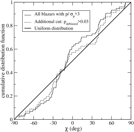
Figure 6: Upper panel: histogram of polarization angles $\chi$ for all sources with $p/\sigma_{p}\geq 3$. The double arrow represents the typical uncertainty on $\chi$; the associated spread in uncertainties is about $10\%$ of that value. Lower panel: cumulative distribution of the polarization angles $\chi$. The PDF and CDF of a uniform $\chi$ distribution are over-plotted in the upper and lower panel respectively with the thick solid line.

In this section we assess the consistency of the measured polarization angles, $\chi$, with an expected uniform distribution. For this reason, we plot in Fig. 6, the histogram (normalised so that it corresponds to a PDF) and the CDF of the polarization angles $\chi$, for all sources with $p/\sigma_{p}\geq 3$ (72 sources). The difference from the (overplotted) uniform distribution is not statistically significant: the maximum difference between the two CDFs is 0.132 and a Kolmogorov–Smirnov test finds the two distributions consistent at the 15 % level. The agreement further improves to the $1\sigma$ level if we only include sources that satisfy the additional requirement that $p>3\times 10^{-2}$ (56 sources, dashed lines in Fig. 6).

The reason for the difference between the uniform distribution and that of the measured $\chi$ when sources with low (but high-significance) $p-$values are included is likely astrophysical. For low polarization sources, any foreground polarization picked up by their optical light during propagation would be a larger fraction of the overall polarization, and any preferred direction in the foreground polarization would affect more significantly the final value of $\chi$. Indeed, half of the sources removed by the $p=3\times 10^{-2}$ have polarization angles covering only a small range of values, between $-20$ and $0$ degrees (close to the maximum of the solid-line histogram in the upper panel of Fig. 6.) This is exactly the behaviour that would be expected from low-level foreground polarization in a preferred direction (see discussion in § 5).

Table 2: Photometric and polarization results of the RoboPol June 2013 optical polarization survey of gamma-ray–loud blazars and the gamma-ray–quiet control sample sources. Note that the polarization angle $\chi$ has been corrected for instrumental rotation of 2.31$\pm$0.34 deg as discussed in “pipeline” paper. The error in the instrumental rotation is accounted for in the final error estimate through formal error propagation. This table is also available electronically as supplementary material.

RoboPol ID

$R^{1}$

$p$

$\chi$

Date4

RoboPol ID

$R^{1}$

$p$

$\chi$

Date4

(mag)

(fraction)

(deg)

(mag)

(fraction)

(deg)

Target Sample

RBPL J0841$+$7053

16.6 $\pm$

0.12

0.020 $\pm$

0.006

$-$19.1 $\pm$

9.0

J24

RBPL J1637$+$4717

18.1 $\pm$

0.1

0.042 $\pm$

0.010

$-$12.3 $\pm$

6.5

J01, J06

RBPL J0848$+$6606

18.2 $\pm$

0.12

0.014 $\pm$

0.021

8.2 $\pm$

43.3

J21

RBPL J1642$+$3948

17.6 $\pm$

0.1

0.031 $\pm$

0.012

61.9 $\pm$

10.9

J08

RBPL J0956$+$2515

17.6 $\pm$

0.1

0.020 $\pm$

0.024

$-$65.3 $\pm$

36.9

J10

RBPL J1643$-$0646

16.9 $\pm$

0.2

0.028 $\pm$

0.015

14.1 $\pm$

15.1

J08

RBPL J0957$+$5522

15.7 $\pm$

0.1

0.057 $\pm$

0.008

4.7 $\pm$

4.2

J25

RBPL J1649$+$5235

17.0 $\pm$

0.5

0.090 $\pm$

0.004

$-$30.8 $\pm$

1.3

J09

RBPL J1014$+$2301

17.0 $\pm$

0.1

0.009 $\pm$

0.010

30.1 $\pm$

31.3

J11

RBPL J1653$+$3945

13.7 $\pm$

0.022

0.027 $\pm$

0.001

1.8 $\pm$

0.8

J01, J27

RBPL J1018$+$3542

17.1 $\pm$

0.1

0.014 $\pm$

0.013

$-$61.5 $\pm$

28.1

J19

RBPL J1722$+$1013

17.6 $\pm$

0.3

0.257 $\pm$

0.022

$-$30.4 $\pm$

2.8

J10, J27

RBPL J1032$+$3738

17.9 $\pm$

0.2

0.098 $\pm$

0.022

47.8 $\pm$

6.3

J25

RBPL J1727$+$4530

17.3 $\pm$

0.2

0.063 $\pm$

0.021

50.4 $\pm$

9.1

J10

RBPL J1037$+$5711

16.2 $\pm$

0.04

0.037 $\pm$

0.005

42.9 $\pm$

3.6

J22, J24

RBPL J1748$+$7005

15.7 $\pm$

0.2

0.160 $\pm$

0.002

67.2 $\pm$

0.5

J19

RBPL J1041$+$0610

16.7 $\pm$

0.12

0.011 $\pm$

0.012

$-$54.4 $\pm$

21.2

J08

RBPL J1749$+$4321

17.4 $\pm$

0.4

0.214 $\pm$

0.012

$-$1.3 $\pm$

1.6

J09

RBPL J1048$+$7143

15.9 $\pm$

0.32

0.070 $\pm$

0.005

$-$44.1 $\pm$

2.1

J24

RBPL J1754$+$3212

16.6 $\pm$

0.3

0.060 $\pm$

0.005

$-$6.0 $\pm$

2.5

J18

RBPL J1054$+$2210

17.7 $\pm$

0.13

0.073 $\pm$

0.013

$-$4.9 $\pm$

5.4

J08

RBPL J1800$+$7828

16.3 $\pm$

0.2

0.047 $\pm$

0.005

$-$72.4 $\pm$

3.2

J21

RBPL J1058$+$5628

14.9 $\pm$

0.33

0.036 $\pm$

0.004

$-$57.0 $\pm$

2.9

J21

RBPL J1806$+$6949

14.2 $\pm$

0.1

0.088 $\pm$

0.002

81.6 $\pm$

0.6

M26, J19

RBPL J1104$+$0730

…

0.149 $\pm$

0.007

38.0 $\pm$

1.4

J09, J25

RBPL J1809$+$2041

19.5 $\pm$

0.8

0.065 $\pm$

0.010

$-$32.2 $\pm$

4.5

J08

RBPL J1121$-$0553

18.4 $\pm$

0.12

0.037 $\pm$

0.038

$-$49.4 $\pm$

30.7

J09

RBPL J1813$+$0615

16.1 $\pm$

0.2

0.161 $\pm$

0.005

39.6 $\pm$

1.0

J12, J24

RBPL J1132$+$0034

17.8 $\pm$

0.1

0.071 $\pm$

0.012

$-$82.5 $\pm$

4.7

J11, J26

RBPL J1813$+$3144

16.1 $\pm$

0.1

0.050 $\pm$

0.004

51.1 $\pm$

2.2

J03, J24

RBPL J1152$-$0841

18.0 $\pm$

0.2

0.007 $\pm$

0.049

$-$62.6 $\pm$

197.1

J11

RBPL J1824$+$5651

15.5 $\pm$

0.1

0.031 $\pm$

0.004

$-$51.9 $\pm$

3.8

M31, J09

RBPL J1203$+$6031

15.6 $\pm$

0.042

0.014 $\pm$

0.005

38.8 $\pm$

10.6

J19

RBPL J1836$+$3136

17.0 $\pm$

0.6

0.120 $\pm$

0.006

$-$23.9 $\pm$

1.4

J08

RBPL J1204$-$0710

16.4 $\pm$

0.4

0.028 $\pm$

0.006

$-$7.8 $\pm$

9.2

J06

RBPL J1838$+$4802

15.6 $\pm$

0.12

0.059 $\pm$

0.003

37.1 $\pm$

1.3

J03

RBPL J1217$+$3007

14.7 $\pm$

0.022

0.109 $\pm$

0.002

$-$11.7 $\pm$

0.5

J22, J24

RBPL J1844$+$5709

17.3 $\pm$

0.2

0.040 $\pm$

0.008

$-$49.7 $\pm$

5.9

J22

RBPL J1220$+$0203

15.3 $\pm$

0.1

0.008 $\pm$

0.003

11.0 $\pm$

10.0

J23

RBPL J1849$+$6705

18.6 $\pm$

0.2

0.066 $\pm$

0.023

13.5 $\pm$

10.1

J20

RBPL J1222$+$0413

18.0 $\pm$

0.12

0.108 $\pm$

0.030

$-$91.2 $\pm$

5.9

J23

RBPL J1903$+$5540

15.7 $\pm$

0.5

0.101 $\pm$

0.003

41.7 $\pm$

0.9

J22

RBPL J1224$+$2436

15.8 $\pm$

0.12

0.089 $\pm$

0.003

21.7 $\pm$

1.1

J23

RBPL J1927$+$6117

17.7 $\pm$

0.63

0.088 $\pm$

0.008

$-$40.6 $\pm$

2.7

J22

RBPL J1230$+$2518

15.0 $\pm$

0.2

0.055 $\pm$

0.002

$-$73.8 $\pm$

0.9

J23

RBPL J1959$+$6508

14.4 $\pm$

0.3

0.052 $\pm$

0.005

$-$25.1 $\pm$

2.5

J20

RBPL J1238$-$1959

16.7 $\pm$

0.2

0.184 $\pm$

0.017

59.9 $\pm$

2.7

J21

RBPL J2000$-$1748

17.5 $\pm$

0.3

0.130 $\pm$

0.025

12.8 $\pm$

5.3

J09

RBPL J1245$+$5709

16.9 $\pm$

0.32

0.169 $\pm$

0.013

9.7 $\pm$

2.1

J22

RBPL J2005$+$7752

15.5 $\pm$

0.3

0.047 $\pm$

0.003

80.8 $\pm$

2.2

J22

RBPL J1248$+$5820

15.0 $\pm$

0.12

0.044 $\pm$

0.003

$-$34.8 $\pm$

2.2

J19

RBPL J2015$-$0137

16.9 $\pm$

0.3

0.149 $\pm$

0.006

59.0 $\pm$

1.3

J09

RBPL J1253$+$5301

16.4 $\pm$

0.022

0.139 $\pm$

0.003

39.8 $\pm$

0.8

J22, J24

RBPL J2016$-$0903

17.1 $\pm$

0.3

0.025 $\pm$

0.008

$-$1.0 $\pm$

8.6

J10

RBPL J1256$-$0547

15.3 $\pm$

0.032

0.232 $\pm$

0.002

39.6 $\pm$

0.4

M30, J23

RBPL J2022$+$7611

16.0 $\pm$

0.1

0.202 $\pm$

0.004

35.2 $\pm$

0.7

J22, J25

RBPL J1337$-$1257

17.7 $\pm$

0.1

0.123 $\pm$

0.026

80.3 $\pm$

5.5

J21

RBPL J2030$-$0622

15.0 $\pm$

0.5

0.014 $\pm$

0.002

$-$17.7 $\pm$

3.8

J10

RBPL J1354$-$1041

16.6 $\pm$

0.2

0.004 $\pm$

0.010

71.9 $\pm$

75.8

J21

RBPL J2030$+$1936

18.2 $\pm$

0.4

0.096 $\pm$

0.014

$-$32.3 $\pm$

4.5

J19

RBPL J1357$+$0128

17.1 $\pm$

0.1

0.137 $\pm$

0.010

$-$10.1 $\pm$

2.1

J24, J26

RBPL J2039$-$1046

17.4 $\pm$

0.2

0.020 $\pm$

0.008

44.6 $\pm$

11.4

J20

RBPL J1419$+$5423

14.6 $\pm$

0.012

0.039 $\pm$

0.003

$-$65.8 $\pm$

1.9

J22

RBPL J2131$-$0915

17.0 $\pm$

0.042

0.082 $\pm$

0.014

71.9 $\pm$

4.7

J24

RBPL J1427$+$2348

13.7 $\pm$

0.042

0.035 $\pm$

0.001

$-$54.6 $\pm$

0.9

M31, J11

RBPL J2143$+$1743

15.8 $\pm$

0.042

0.020 $\pm$

0.003

$-$4.3 $\pm$

4.5

J10

RBPL J1510$-$0543

17.1 $\pm$

0.022

0.014 $\pm$

0.010

39.6 $\pm$

21.8

J11

RBPL J2146$-$1525

17.0 $\pm$

0.1

0.028 $\pm$

0.018

55.5 $\pm$

19.1

J24

RBPL J1512$-$0905

15.9 $\pm$

0.3

0.028 $\pm$

0.006

29.9 $\pm$

6.2

J11

RBPL J2147$+$0929

18.4 $\pm$

0.22

0.037 $\pm$

0.020

48.8 $\pm$

16.8

J19

RBPL J1512$+$0203

16.7 $\pm$

0.12

0.079 $\pm$

0.007

$-$29.4 $\pm$

2.7

J11

RBPL J2148$+$0657

15.7 $\pm$

0.022

0.013 $\pm$

0.003

13.7 $\pm$

5.9

J10, J23

RBPL J1516$+$1932

18.2 $\pm$

0.12

0.012 $\pm$

0.020

72.2 $\pm$

46.1

J06

RBPL J2149$+$0322

15.6 $\pm$

0.1

0.120 $\pm$

0.023

50.6 $\pm$

11.2

J11

RBPL J1542$+$6129

14.8 $\pm$

0.032

0.092 $\pm$

0.003

$-$25.1 $\pm$

1.0

J19

RBPL J2202$+$4216

14.0 $\pm$

0.012

0.085 $\pm$

0.001

$-$11.3 $\pm$

0.5

J19, J26

RBPL J1548$-$2251

15.8 $\pm$

0.5

0.027 $\pm$

0.011

$-$69.0 $\pm$

11.6

J11

RBPL J2217$+$2421

17.9 $\pm$

0.1

0.183 $\pm$

0.016

$-$24.9 $\pm$

2.5

J19

RBPL J1550$+$0527

18.1 $\pm$

0.2

0.039 $\pm$

0.021

$-$42.9 $\pm$

17.1

J10, J26

RBPL J2232$+$1143

16.2 $\pm$

0.22

0.063 $\pm$

0.005

$-$7.0 $\pm$

1.9

J23

RBPL J1555$+$1111

14.2 $\pm$

0.12

0.030 $\pm$

0.002

$-$61.3 $\pm$

1.7

M31, J10

RBPL J2253$+$1608

15.2 $\pm$

0.1

0.012 $\pm$

0.007

$-$39.6 $\pm$

16.1

J21

RBPL J1558$+$5625

17.0 $\pm$

0.5

0.071 $\pm$

0.007

$-$19.7 $\pm$

2.8

J09

RBPL J2321$+$2732

18.6 $\pm$

0.052

0.043 $\pm$

0.026

$-$10.9 $\pm$

16.4

J23, J25

RBPL J1604$+$5714

17.8 $\pm$

0.12

0.028 $\pm$

0.010

$-$26.8 $\pm$

10.6

J19

RBPL J2325$+$3957

17.0 $\pm$

0.5

0.036 $\pm$

0.033

21.6 $\pm$

26.5

J22

RBPL J1608$+$1029

18.1 $\pm$

0.12

0.017 $\pm$

0.024

72.2 $\pm$

39.6

M31, J11

RBPL J2340$+$8015

16.6 $\pm$

0.4

0.093 $\pm$

0.008

$-$36.2 $\pm$

2.7

J21

RBPL J1635$+$3808

16.5 $\pm$

0.012

0.022 $\pm$

0.004

$-$7.7 $\pm$

5.3

M31, J06

Control Sample Candidates

J0017$+$8135

16.4 $\pm$

0.6

0.011 $\pm$

0.005

72.0 $\pm$

13.0

J23

J1603$+$5730

17.0 $\pm$

0.01

0.018 $\pm$

0.006

$-$7.7 $\pm$

10.0

J25

J0702$+$8549

18.3 $\pm$

0.3

0.011 $\pm$

0.013

$-$31.3 $\pm$

35.6

J26

J1623$+$6624

18.2 $\pm$

0.5

0.032 $\pm$

0.013

$-$36.1 $\pm$

10.9

J25

J1010$+$8250

16.2 $\pm$

0.4

0.098 $\pm$

0.011

$-$19.0 $\pm$

3.3

J26

J1624$+$5652

17.7 $\pm$

0.1

0.146 $\pm$

0.010

40.8 $\pm$

1.9

J25

J1017$+$6116

16.4 $\pm$

0.3

0.015 $\pm$

0.020

$-$37.2 $\pm$

40.0

J25

J1638$+$5720

16.5 $\pm$

0.2

0.013 $\pm$

0.003

$-$20.7 $\pm$

7.6

J26

J1148$+$5924

13.8 $\pm$

0.02

0.025 $\pm$

0.001

12.9 $\pm$

1.4

J25

J1854$+$7351

16.3 $\pm$

0.2

0.020 $\pm$

0.004

$-$22.0 $\pm$

5.1

J26

J1436$+$6336

15.8 $\pm$

0.6

0.012 $\pm$

0.004

$-$7.5 $\pm$

10.5

J25

J1927$+$7358

15.6 $\pm$

0.1

0.021 $\pm$

0.005

$-$30.2 $\pm$

6.5

J25

J1526$+$6650

17.3 $\pm$

0.2

0.013 $\pm$

0.012

$-$43.6 $\pm$

27.1

J27

J2042$+$7508

14.3 $\pm$

0.2

0.018 $\pm$

0.001

$-$9.6 $\pm$

1.7

J23

J1551$+$5806

16.7 $\pm$

0.04

0.025 $\pm$

0.005

$-$25.5 $\pm$

5.6

J25

¹photometry based on USNO-B1.0 R2 unless otherwise noted

²photometry based on PTF

³photometry based on USNO-B1.0 R1

⁴Day of June 2013 (JXX) or May 2013 (MXX) in which the observation took place. In cases of multiple measurements we report the dates of the first and the last observations, respectively.

5 Summary and Discussion

We have presented first results from RoboPol, including a linear polarization survey of a sample of 89 gamma-ray–loud blazars, and a smaller sample of 15 gamma-ray–quiet blazars defined according to objective selection criteria, easily reproducible in simulations, and additional unbiased cuts (due to scheduling and quality of observations, independent of source properties). These results are therefore representative of the gamma-ray–loud and gamma-ray–quiet blazar populations, and as such are appropriate for populations studies.

Our findings can be summarised as follows:

• The hypothesis that the polarization fractions of gamma-ray–loud and gamma-ray quiet blazars are drawn from the same distribution is rejected at the $3\sigma$ level.

• The probability distribution functions of polarization fraction of gamma-ray–loud and gamma-ray–quiet blazars can be well described by exponential distributions.

• Using a likelihood analysis we estimate the best-estimate values and $1\sigma$ uncertainties of the mean polarization fraction of each subpopulation, which is the single parameter characterising an exponential distribution. We find $\langle p\rangle=6.4^{+0.9}_{-0.8}\times 10^{-2}$ for gamma-ray–loud blazars, and $\langle p\rangle=3.2^{+2.0}_{-1.1}\times 10^{-2}$ for gamma-ray–quiet blazars.

• The large upwards uncertainty of $\langle p\rangle$ for gamma-ray–quiet blazars is a side-effect of the strict cuts we have applied in our likelihood analysis, leaving us only with 7 useable sources for the gamma-ray–quiet sample. This is the reason why the statistical inconsistency between the two populations cannot be also verified with this method. This problem can be improved with a larger gamma-ray–quiet blazar survey, longer integration times, and a more sophisticated analysis.

• Polarization angles, $\chi$, for blazars in our survey are consistent with being drawn from a uniform distribution.

It is the first time a statistical difference between the average polarization properties of gamma-ray–quiet and gamma-ray–loud blazars is demonstrated in optical wavelengths. The difference is consistent with the findings of Hovatta et al. (2010) for the radio polarization of gamma-ray–loud and, otherwise similar, gamma-ray–quiet sources. It thus appears that the gamma-ray–loud blazars overall exhibit higher degree of polarization in their synchrotron emission than their gamma-ray–quiet counterparts. One interpretation for this finding may involve the degree of uniformity of the magnetic field over the emission region, which is an important factor affecting the degree of polarization. The bulk of synchrotron in gamma-ray–loud blazars might therefore originate in regions of higher magnetic field uniformity than the emission from gamma-ray–quiet blazars. It is possible that shocks that are strong/persistent enough to accelerate particles capable of gamma-ray emission are also better in locally aligning magnetic field lines and producing regions of high field uniformity, hence a higher polarization degree.

We have found hints of depolarization at high optical fluxes, an effect that may be attributable to the contribution of unpolarized light to the overall flux by the blazar’s host galaxy. The statistics of BL Lac hosts at least are consistent with this idea: in about $50\%$ of the sources studied by Nilsson et al. (2003) the host would have a contribution of more than 50% the core flux inside our typical aperture. We will examine the effect quantitatively and in more detail using our full first season data in an upcoming publication.

Inclusion of sources of low (but significantly measured) polarization fraction in the empirical distribution of polarization angles generates some tension (although still not statistically significant) between that distribution and an expected uniform one. This may be a result of foreground polarization at a preferred direction, which, although small and not important for high-polarization sources, tends to align lower polarization sources. Although the sources in the RoboPol sample have been selected to lie away from the Galactic plane so foreground polarization due to interstellar dust absorption should be at a minimum, nearby interstellar material might also induce some degree of foreground polarization. For example, such an effect, at the $p\sim 0.8\times 10^{-2}$ level, has been seen in the southern sky by Santos et al. (2013). A similar level of foreground polarization, $p\sim 0.9\times 10^{-2}$, has been suggested by Sillanpää et al. (1993) for the vicinity of BL Lac (which however lies at relatively low Galactic latitude $b\sim-10^{\circ}$). A cut at $p>3\times 10^{-2}$ ensures that sources are intrinsically at least twice as polarized as that, so the effect in measured $\chi$ is minimised. Because the $13^{\prime}\times 13^{\prime}$ fields around sources in our monitoring program accumulate exposure during our observing season, we will be eventually able to measure the polarization properties of non-variable, intrinsically unpolarized sources induced by foregrounds to higher accuracy, and better study and correct for this effect in the future.

For the remainder of the 2013 season we have been monitoring a 3-element sample in linear polarization with RoboPol: an unbiased gamma-ray–loud blazar sample (51 sources); a smaller, again unbiased, gamma-ray–quiet sample (10 sources); and a list of high-interest sources that have not made our cuts (24 sources). After the end of the 2013 season, we will present first light curves and analysis of our sources in terms of polarization variability and cross-correlations in the amplitude and time domains. Finally, we will revisit our monitoring sample definition, to strengthen the robustness of criteria (for example, using RoboPol average R-band fluxes for the $R$ magnitude cuts), and to develop our automatic scheduling algorithm which aims to self-trigger high cadence observations during polarization changes that are unusually fast for a specific source. In this way, we aim to better constrain the linear polarization properties of the blazar population at optical wavelengths and to provide a definitive answer to whether a significant fraction of fast polarization rotations do indeed coincide with gamma-ray flares.

Table 3: Additional archival information for the 89 high quality sources as well as the control sample ones. The table presents only the first 5 lines of the full table which is available online as supplementary material. The column numbers correspond to individual columns in the online version of the table.

1

2

3

4

56

7

8

9 $\pm$ 10

11${}_{-12}^{+13}$

14

15$\pm$16

17

18

ROBOPOL ID

Survey ID

RA

DEC

z

Class

Programs

$\left<S_{15}\right>_{6-8}$

$m$

$F\left(>100\,\rm{MeV}\right)$

$\Gamma$

VI

In CGRaBS

(J2000)

(J2000)

(Jy)

(fraction)

($10^{-8}\,\rm{cm}^{-2}\,\rm{s}^{-1}$)

RBPLJ0841$+$7053

4C $+$71.07

08h41m24.2s

$+$70d53m41.9s

2.2184

BZQ

O, T, F1,2

2.337$\pm$0.018

…

6.0

2.95$\pm$0.07

91.5

0

RBPLJ0848$+$6606

GB6 J0848+6605

08h48m54.6s

$+$66d06m09.6s

…

BZ?

O

0.020$\pm$0.002

…

2.0

1.96$\pm$0.16

33.0

0

RBPLJ0956$+$2515

OK 290

09h56m49.8s

$+$25d15m15.9s

0.7082

BZQ

O

1.377$\pm$0.022

0.192${}_{-0.009}^{+0.009}$

2.5

2.39$\pm$0.07

84.7

1

RBPLJ0957$+$5522

4C $+$55.17

09h57m38.1s

$+$55d22m57.0s

0.8964

BZQ

O, T

1.166$\pm$0.007

0.028${}_{-0.003}^{+0.003}$

8.4

1.83$\pm$0.03

23.4

0

RBPLJ1014$+$2301

4C $+$23.24

10h14m46.9s

$+$23d01m15.9s

0.5655

BZQ

O

1.246$\pm$0.005

0.085${}_{-0.004}^{+0.004}$

2.4

2.54$\pm$0.16

33.0

1

Column Description: 1: The RoboPol identification name – 2: A common survey name – 3, 4: RA, DEC – 5: redshift – 6: reference for the redshift – 7: BZCAT Class as of November 14, 2013 with “BZB” denoting BL Lac objects, “BZ?” BL Lac candidates, “BZQ” flat-spectrum radio quasars and “BZU” blazars of uncertain type – 8: other monitoring programs with “O” for OVRO 15 GHz, “T” Torun 30 GHz and F1 and F2 F-GAMMA monitoring before or after June 2009 – 9: Flux Density at 15 GHz averaged over June-August 2013 – 10 its uncertainty – 11: The intrinsic modulation index as computed by Richards et al. 2011 – 12, 13: the lower and upper uncertainty – 14: Photon Flux above 100 MeV – 15, 16: The spectral index and its uncertainty as given in the 2FGL – 17: the variability index as given in the 2FGL – 18: Flag indicating whether the source is in the CGRaBS catalog.
¹Shaw et al. (2013)
²Shaw et al. (2012)
³Ackermann et al. (2011)
⁴Abdo & et al. (2010)
⁵Healey et al. (2008)
⁶M. Shaw, personal comm.

References

- Abdo & et al. (2010) Abdo A. A., et al., 2010, ApJ, 715, 429
- Abdo et al. (2010) Abdo A. A., Ackermann M., Ajello M., et al., 2010, Nature, 463, 919
- Ackermann et al. (2011) Ackermann M. et al., 2011, ApJ, 743, 171
- Angelakis et al. (2010) Angelakis E., Fuhrmann L., Nestoras I., Zensus J. A., Marchili N., Pavlidou V., Krichbaum T. P., 2010, ArXiv e-prints 1006.5610
- Atwood et al. (2009) Atwood W. B., Abdo A. A., Ackermann M., et al., 2009, ApJ, 697, 1071
- Baixeras et al. (2004) Baixeras C., Bastieri D., Bigongiari C., et al., 2004, Nuclear Instruments and Methods in Physics Research A, 518, 188
- Blandford & Königl (1979) Blandford R. D., Königl A., 1979, ApJ, 232, 34
- Browne et al. (2000) Browne I. W., Mao S., Wilkinson P. N., Kus A. J., Marecki A., Birkinshaw M., 2000, in Society of Photo-Optical Instrumentation Engineers (SPIE) Conference Series, Vol. 4015, Society of Photo-Optical Instrumentation Engineers (SPIE) Conference Series, Butcher H. R., ed., pp. 299–307
- Fuhrmann et al. (2007) Fuhrmann L., Zensus J. A., Krichbaum T. P., Angelakis E., Readhead A. C. S., 2007, in American Institute of Physics Conference Series, Vol. 921, The First GLAST Symposium, Ritz S., Michelson P., Meegan C. A., eds., pp. 249–251
- Giommi et al. (2012) Giommi P., Polenta G., Lähteenmäki A., et al., 2012, Astronomy and Astrophysics, 541, A160
- Hagen-Thorn et al. (2006) Hagen-Thorn V. A., Larionov V. M., Efimova N. V., et al., 2006, Astronomy Reports, 50, 458
- Healey et al. (2008a) Healey S. E., Romani R. W., Cotter G., et al., 2008a, ApJS, 175, 97
- Healey et al. (2008) Healey S. E. et al., 2008, ApJS, 175, 97
- Hovatta et al. (2010) Hovatta T., Lister M. L., Kovalev Y. Y., Pushkarev A. B., Savolainen T., 2010, International Journal of Modern Physics D, 19, 943
- Ikejiri et al. (2011) Ikejiri Y., Uemura M., Sasada M., et al., 2011, PASJ, 63, 639
- King et al. (2013) King O. G., Blinov D., Ramaprakash A. N., et al., 2013, MNRAS in press, ArXiv e-prints 1310.7555
- Lasker et al. (2008) Lasker B. M., Lattanzi M. G., McLean B. J., et al., 2008, AJ, 136, 735
- Marscher et al. (2008) Marscher A. P., Jorstad S. G., D’Arcangelo F. D., et al., 2008, Nature, 452, 966
- Massaro et al. (2009) Massaro E., Giommi P., Leto C., Marchegiani P., Maselli A., Perri M., Piranomonte S., Sclavi S., 2009, VizieR Online Data Catalog, 349, 50691
- Monet et al. (2003) Monet D. G., Levine S. E., Canzian B., et al., 2003, The Astronomical Journal, 125, 984
- Nilsson et al. (2003) Nilsson K., Pursimo T., Heidt J., Takalo L. O., Sillanpää A., Brinkmann W., 2003, A&A, 400, 95
- Nolan et al. (2012) Nolan P. L. et al., 2012, ApJS, 199, 31
- Ofek et al. (2012) Ofek E. O., Laher R., Surace J., et al., 2012, Publications of the Astronomical Society of the Pacific, 124, 854
- Papamastorakis (2007) Papamastorakis Y., 2007, Ipparchos, 2, 14
- Peel et al. (2011) Peel M. W. et al., 2011, MNRAS, 410, 2690
- Richards et al. (2011) Richards J. L., Max-Moerbeck W., Pavlidou V., et al., 2011, ApJS, 194, 29
- Santos et al. (2013) Santos F. P., Franco G. A. P., Roman-Lopes A., Reis W., Román-Zúñiga C. G., 2013, ArXiv e-prints 1310.7037
- Sazonov (1972) Sazonov V. N., 1972, Astrophysics and Space Science, 19, 25
- Shaw et al. (2012) Shaw M. S. et al., 2012, ApJ, 748, 49
- Shaw et al. (2013) Shaw M. S. et al., 2013, ApJ, 764, 135
- Sillanpää et al. (1993) Sillanpää A., Takalo L. O., Nilsson K., Kikuchi S., 1993, ApSS, 206, 55
- Simmons & Stewart (1985) Simmons, J. F. L., & Stewart, B. G. 1985, A&A, 142, 100
- Smith et al. (2009) Smith P. S., Montiel E., Rightley S., Turner J., Schmidt G. D., Jannuzi B. T., 2009, ArXiv e-prints 0912.3621
- Souchay et al. (2011) Souchay J., Andrei A. H., Barache C., Bouquillon S., Suchet D., Taris F., Peralta R., 2011, VizieR Online Data Catalog, 353, 79099
- Vaillancourt (2006) Vaillancourt J. E., 2006, PASP, 118, 1340