Clustering in the Phase Space of Dark Matter Haloes. II. Stable Clustering and Dark Matter Annihilation

Abstract

We present a model for the structure of the particle phase space average density ($P^{2}SAD$) in galactic haloes, introduced recently as a novel measure of the clustering of dark matter. Our model is based on the stable clustering hypothesis in phase space, the spherical collapse model, and tidal disruption of substructures, which is calibrated against the Aquarius simulations. Using this model, we can predict the behaviour of $P^{2}SAD$ in the numerically unresolved regime, down to the decoupling mass limit of generic WIMP models. This prediction can be used to estimate signals sensitive to the small scale structure of dark matter. For example, the dark matter annihilation rate can be estimated for arbitrary velocity-dependent cross sections in a convenient way using a limit of $P^{2}SAD$ to zero separation in physical space. We illustrate our method by computing the global and local subhalo annihilation boost to that of the smooth dark matter distribution in a Milky-Way-size halo. Two cases are considered, one where the cross section is velocity independent and one that approximates Sommerfeld-enhanced models. We find that the global boost is $\sim 10-30$, which is at the low end of current estimates (weakening expectations of large extragalactic signals), while the boost at the solar radius is below the percent level. We make our code to compute $P^{2}SAD$ publicly available, which can be used to estimate various observables that probe the nanostructure of dark matter haloes.

1 Introduction

Despite being the most dominant type of matter in the Universe, dark matter is evident so far only through its gravitational effects on luminous matter. The nature of dark matter will thus continue to be elusive unless it has detectable non-gravitational interactions. Weakly Interacting Massive Particles (WIMPs) are among the favourite dark matter candidates and are expected to give promising signals that can be detected experimentally either directly through scattering off nuclei in laboratory detectors, or indirectly through the byproducts of their self-annihilation into standard model particles (e.g. photons and electron/positrons pairs). Several experiments are pursuing such a discovery and their sensitivity is reaching the level of interaction predicted by popular WIMP models (e.g. Abazajian et al., 2012; Aprile et al., 2012).

Interestingly, there are tantalizing anomalies that might be caused by new dark matter physics. For instance, although the excess of $>10$ GeV cosmic ray positrons established firmly by the PAMELA and Fermi Satellites (Adriani et al., 2009; Abdo et al., 2009), and recently confirmed with high precision by the AMS collaboration (Aguilar et al., 2013), can be explained by “ordinary” astrophysical sources (e.g. nearby pulsars, Linden & Profumo 2013), it can also be interpreted as dark matter annihilation. Large annihilation rates, of $\mathcal{O}(100-1000)$ above the expected rate of a $\sim$TeV mass thermal relic, and primarily leptonic final states are needed, however, to explain the data (Bergström et al., 2009). These requirements can be satisfied by leptophilic dark matter models coupled to light force carriers that enhance the annihilation cross section via a Sommerfeld mechanism (e.g. Arkani-Hamed et al., 2009; Pospelov & Ritz, 2009). An anomalous extended gamma-ray emission at intermediate galactic latitudes (peaking at $1$ GeV) has also been interpreted as a signal of dark matter annihilation (e.g. Hooper & Slatyer, 2013).

Predictions for the hypothetical non-gravitational signatures of dark matter are highly dependent on the clustering of dark matter at small scales. Although the steady progress of numerical $N-$body simulations over the past few decades has given us a detailed picture of the spatial dark matter distribution from large ($\sim$ Gpc) to sub-galactic scales ($\sim 100$ pc), the regime most relevant for certain dark matter detection efforts (those based on extragalactic signals) remains below the resolution of current simulations ($\mathcal{O}(10^{3}$M_⊙) at $z=0$; Springel et al. 2008; Diemand et al. 2008; Stadel et al. 2009). This is because the current cold dark matter (CDM) paradigm of structure formation predicts a hierarchical scenario with a very large mass range of gravitationally bound dark matter structures, from $10^{15}$M_⊙ cluster-size haloes down to a decoupling mass limit of $10^{-11}-10^{-3}$M_⊙ (e.g. Bringmann, 2009). The characteristic sizes of these small haloes (commonly called microhaloes) varies from $\sim 10^{-7}-10^{-10}$ times the size of a Milky Way (MW) type halo (we call this the nanostructure of dark matter haloes).

Despite their limited resolution, current simulations clearly suggest that the contribution of low-mass (sub)haloes is dominant for dark matter annihilation signals in the case of extragalactic sources, such as gamma-rays from galaxy clusters (e.g. Gao et al., 2012) and from integrated backgrounds (e.g. Zavala et al., 2010; Fornasa et al., 2013). Within the solar radius, it seems that the dominant signal should come from the diffuse distribution of dark matter rather than by small scale subclumps (Springel et al., 2008). Substructures within the MW halo can be detected in gamma-rays either individually as the hosts of satellite galaxies (Ackermann et al., 2011), dark satellites devoid of stars (Ackermann et al., 2012) or as a dominant contribution to the angular power spectrum of a full-sky gamma-ray signal (e.g. Siegal-Gaskins, 2008).

Extrapolations below resolved scales are therefore needed to obtain a prediction of the expected signals from dark matter annihilation. For a given host halo, these extrapolations ultimately depend on the survivability of the smallest substructures as they are tidally disrupted by the host. Low mass subhaloes form earlier in the hierarchical scenario and, being the densest, are expected to survive tidal disruption contributing heavily to the annihilation signal. Current estimates on this contribution mostly rely on assumptions about the abundance, spatial distribution, and internal properties of unresolved subhaloes that could lead to significant over/underestimations. Typical estimates calibrated to simulation data vary by up to an order of magnitude (e.g. Springel et al., 2008; Kuhlen et al., 2008; Kamionkowski et al., 2010). The role of substructure, and therefore the uncertainty in the extrapolations to the unresolved regime, is magnified in Sommerfeld-enhanced models where the annihilation cross section scales as the inverse velocity making the cold and dense subhaloes dominant not only in extragalactic structures (Zavala et al., 2011) but plausibly also locally (Slatyer et al., 2012).

In this paper, we present a novel method to study dark matter clustering that can be used to estimate the dark matter annihilation rate calibrated with simulation data. This method is based on a physically-motivated model inspired by an extension into phase space of the stable clustering hypothesis (Afshordi et al., 2010), originally introduced in position space by Davis & Peebles (1977). The novelty of the method relies on using a more complete picture of dark matter clustering based on a new quantity, the particle phase space average density ($P^{2}SAD$), a coarse-grained phase space density that can be used straightforwardly to compute the annihilation rate. $P^{2}SAD$ was introduced in a companion paper (Zavala & Afshordi, 2013, hereafter Paper I) where we studied its main features in galactic-size haloes using the simulation suite from the Aquarius project (Springel et al., 2008). Remarkably, we found it to be nearly universal at small scales (i.e. small separations in phase space) across time and in regions of substantially different ambient densities. This near universality is also preserved across the different Aquarius haloes, having similar masses but diverse mass accretion histories: they possess only slightly different $P^{2}SAD$s at small scales without any re-scaling. We argue in this paper that this behaviour can be roughly described by a refinement of the stable clustering hypothesis through a simple model that incorporates tidal disruption of substructures.

In cases other than s-wave self-annihilation, the dependence of the interaction on the relative velocity of the annihilating particles has to be averaged over the velocity distribution of the dark matter particles. Although it is common to assume a Maxwellian velocity distribution, current simulations have shown that there are significant deviations from this assumption related to the dark matter assembly history (e.g. Vogelsberger et al., 2009). Our method is particularly useful for models where the cross section is velocity dependent (such as in Sommerfeld-enhanced models) because the particle phase space average density ($P^{2}SAD$) that we introduce does not rely on assumptions about the velocity distribution and can deal with these cases in a natural way.

This paper is organised as follows: In Section 2, we summarize the main results of Paper I, introducing the clustering of dark matter through $P^{2}SAD$ and its nearly universal structure at small scales in galactic haloes. In Section 3, we describe how the annihilation rate is directly connected to the limit of zero physical separation of $P^{2}SAD$. In Section 4, we describe our model of the small scale structure of $P^{2}SAD$ based on the spherical collapse model and the stable clustering hypothesis in phase space, refined by a subhalo tidal disruption prescription. In Section 5, we fit our model to the simulation data while in Section 6 we illustrate how this can be used to compute the global and local subhalo boost to the smooth annihilation rate in a MW-size halo. Finally, a summary and our main conclusions are given in Section 7.

2 The Particle Phase Space Average Density ($P^{2}SAD$) on small scales

We follow the same definitions as in Paper I and study the clustering in phase space through $P^{2}SAD$, defined as the mass-weighted average (over a volume ${\cal V}_{6}$ in phase space) of the coarse-grained phase space density of dark matter, on spheres of radius $\Delta x$ and $\Delta v$, in position and velocity spaces, respectively:

$$\Xi(\Delta x,\Delta v)\equiv\frac{\int_{{\cal V}_{6}}d^{3}{\bf x}d^{3}{\bf v}f({\bf x},{\bf v})f({\bf x}+{\bf\Delta x},{\bf v}+{\bf\Delta v})}{\int_{{\cal V}_{6}}d^{3}{\bf x}d^{3}{\bf v}f({\bf x},{\bf v})}$$ (1)

where $f({\bf x},{\bf v})$ is the phase space distribution function at the phase space coordinates $\bf x$ and $\bf v$.

In Paper I of this series we implemented and tested an estimator of $P^{2}SAD$ in $N-$body simulations based on pair counts and applied to the set of Aquarius haloes (Springel et al., 2008). In this paper, we refer exclusively to the results found for halo Aq-A-2 that has a virial mass and radius, defined with a mean overdensity of 200 times the critical value, of $1.8\times 10^{12}~{}$M_⊙ and $246$ kpc, respectively.

One of the main results that we obtained is that the structure of $P^{2}SAD$ averaged within the virialized halo is clearly separated by two regimes: (i) a region at large scales (i.e. large separations in phase space) dominated by the smooth dark matter distribution where $P^{2}SAD$ varies in time due to the inside-out growth of the dark matter halo, and (ii) a region at small scales (i.e. small separations in phase space) dominated by gravitationally bound substructures where $P^{2}SAD$ is nearly universal across time and ambient density. In the reminder of this paper we consider only the small scale regime, which is the one of relevance in estimating the impact of substructure on dark matter annihilation signals.

Figure 1: Contours of the logarithm of the particle phase space average density ($P^{2}SAD$) of the Aq-A-2 halo (solid) at $z=0$ and for the fitting function defined in Eqs. (2-3) (dashed) with the parameters as given in Table 1. The dashed region in the left corner encompasses the region where resolution is a potential issue (see Appendix of Paper I).

Although the small scale regime can be roughly described by a subhalo model with abundance and properties given by scaling laws fitted to the simulation data (see Fig. 5 of Paper I), we found that a better description is given by a family of superellipse contours of constant $P^{2}SAD$$\equiv\Xi$, with parameters that can be adjusted to fit the variations of $P^{2}SAD$ in redshift and halo-centric distance (see Tables 2 and 3 of Paper I):

$$\left(\frac{\Delta x}{\mathcal{X}(\Xi)}\right)^{\beta}+\left(\frac{\Delta v}{\mathcal{V}(\Xi)}\right)^{\beta}=1,$$ (2)

where $\beta(z;r)$ is a shape parameter and $\mathcal{X}(\Xi)$ and $\mathcal{V}(\Xi)$ are the axes of the superellipse:

$$\mathcal{X}(\Xi)=q_{X}(z;r)\Xi^{\alpha_{X}(z;r)}$$ (3)

$$\mathcal{V}(\Xi)=q_{V}(z;r)\Xi^{\alpha_{V}(z;r)}$$

Fig. 1 shows contours of log($P^{2}SAD$) in the small scale regime averaged within the virialized region of Aq-A-2 at $z=0$ (solid lines). The dotted lines are the fitting contours through Eqs. (2-3) with the parameters as given in Table 1. In section 4, we present the model that motivates this fitting formula. We note that the shaded area on the left corner encompasses the region where our results could be affected by resolution conservatively by $50\%$ at the most (see Appendix of Paper I); we exclude this region from the fitting procedures and from subsequent analyses.

Redshift	$q_{X}({\rm Mpc}/h)$	$\alpha_{X}$	$q_{V}({\rm km/s})$	$\alpha_{V}$	$\beta$
0.0	$11.82$	$-0.4$	$4.5\times 10^{4}$	$-0.33$	$0.75$

Table 1: Values of the fitting parameters in Eq. (3) at $z=0$ over the virialized region of the Aq-A-2 halo. Together with Eqs. (2) and (3), these parameters provide a good description of $P^{2}SAD$ at small $(\Delta x,\Delta v)$ (see Fig. 1).

3 Dark matter annihilation rate: substructure boost

The number of dark matter self-annihilation events per unit time is given in terms of the phase space distribution at the phase space coordinates ${\bf x},{\bf v}$ and ${\bf x}+{\bf\Delta x},{\bf v}+{\bf\Delta v}$:

$$R_{\rm ann} = \frac{1}{2m_{\chi}^{2}}\lim_{\Delta x\to 0}\left[\int d^{3}{\bf\Delta v}\bigg{(}\int_{{\cal V}_{6}}d^{3}{\bf v}d^{3}{\bf x}\right.$$ (4)

$$(\sigma_{\rm ann}v)f({\bf x},{\bf v})f({\bf x}+{\bf\Delta x},{\bf v}+{\bf\Delta v})\bigg{)}\bigg{]}$$

$$= \frac{M_{{\cal V}_{6}}}{2m_{\chi}^{2}}\int d^{3}{\bf\Delta v}(\sigma_{\rm ann}v)\lim_{\Delta x\to 0}\Xi(\Delta x,\Delta v)$$

where $M_{{\cal V}_{6}}$ is the total dark matter mass within the phase space volume ${\cal V}_{6}$, $(\sigma_{\rm ann}v)$ is the product of the annihilation cross section and the relative velocity between pairs, and we have used Eq.(1) to introduce $P^{2}SAD$.

The annihilation rate in a region of spatial volume $V$ is typically written as:

$$R_{\rm ann}=\frac{1}{2m_{\chi}^{2}}\int_{V}d^{3}{\bf x}\rho^{2}({\bf x})\langle\sigma_{\rm ann}v\rangle$$ (5)

where $m_{\chi}$ is the dark matter particle mass, $\rho_{\chi}({\bf x})$ is the local dark matter density (that includes contribution from the smooth dark matter distribution and from substructure), and $\langle\sigma_{\rm ann}v\rangle$ is an average of $(\sigma_{\rm ann}v)$ over the velocity distribution of the dark matter particles (typically assumed to be Maxwellian). Instead of separating the dark matter spatial and velocity distributions, Eq. (4) gives directly, without any assumptions, the annihilation rate as an integral over the relative velocity $\Delta v$ at the limit of zero spatial separation of $P^{2}SAD$, henceforth abbreviated $P^{2}SAD^{\rm zero}$($\Xi^{\rm zero}$). Since in general $(\sigma_{\rm ann}v)$ is an arbitrary function of $\Delta v$, we can use Eq. (4) to easily accommodate any velocity dependent annihilation cross section. Notice also that Eq. (4) adapts to the region of interest for the annihilation rate by simply using $P^{2}SAD$ averaged over that region.

The near universality of $P^{2}SAD$ at small scales (i.e. small separations in phase space) makes the functional shape in Eqs. (2-3) valid across regions of substantially different ambient density with only slight changes to the fitting parameters (see sections 3.3 and 3.4 of Paper I) and can therefore be straightforwardly applied in Eq. (4) to calculate the annihilation rate in gravitationally bound substructure either globally in the whole halo, or locally in a certain region of the halo. Since we also found that at small scales $P^{2}SAD$ is nearly insensitive to the assembly history of a particular halo (see Fig. 10 of Paper I), the results we find for the particular initial conditions of Aq-A-2 are also a very good approximation for different initial conditions.

The integral in Eq. (4) can also be easily transformed into an integral over $P^{2}SAD^{\rm zero}$ using Eq. (2) and a change of variables:

$$R_{\rm ann}=\frac{2\pi M_{{\cal V}_{6}}}{m_{\chi}^{2}}q_{V}^{3}\alpha_{V}\int_{\Xi^{\rm zero}_{\rm max}}^{\Xi^{\rm zero}_{\rm min}}d\Xi^{\rm zero}(\sigma_{\rm ann}v)[\Xi^{\rm zero}]^{3\alpha_{V}}$$ (6)

Notice that because of the limit $\Delta x\rightarrow 0$, the annihilation rate is at the end only sensitive to $\alpha_{V}$ and $q_{V}$. The limits of the integral over $P^{2}SAD^{\rm zero}$ ($\Xi^{\rm zero}_{\rm max(min)}$) correspond to the maximum and minimum values of the separation in velocity where substructures contribute. Note that we can only use Eqs. (2-3) down to:

$$\Xi^{\rm zero}_{\rm min}=\frac{10^{8}{\rm M}_{\odot}}{{\rm Mpc}^{3}({\rm km/s})^{3}}~{}h^{2},$$ (7)

below which $P^{2}SAD^{\rm zero}$ falls off more rapidly than the power law in Eq. (3), and more importantly, the smooth distribution of dark matter dominates $P^{2}SAD$ in general (Paper I). We will then take this value as the transition between the smooth and subhaloes dominance of the annihilation rate.

To compute the contribution from the smooth component we substitute $\rho$ in Eq. (5) by $\rho_{E}$, the spherically averaged Einasto density profile:

$$\rho(r)=\rho_{-2}{\rm exp}\left(\frac{-2}{\alpha_{e}}\left[\left(\frac{r}{r_{-2}}\right)^{\alpha_{e}}-1\right]\right)$$ (8)

where $\rho_{-2}$ and $r_{-2}$ are the density and radius at the point where the logarithmic density slope is -2, and $\alpha_{e}$ is the Einasto shape parameter. We take the parameter values from the fit to the Aq-A-2 halo given in Navarro et al. (2010): $\alpha_{e}=0.163$, $\rho_{-2}=3.9\times 10^{15}~{}{\rm M}_{\odot}/{\rm Mpc}^{3}$, $r_{-2}=15.27~{}{\rm kpc}$. We also assume that the velocity distribution of dark matter particles in the smooth component is Maxwellian. The substructure boost is then simply defined as:

$$B_{{\cal V}_{6}}=\frac{R_{\rm ann}^{\rm subs}}{R_{\rm ann}^{\rm smooth}}=\frac{M_{{\cal V}_{6}}\int d^{3}{\bf\Delta v}(\sigma_{\rm ann}v)\lim_{\Delta x\to 0}\Xi^{\rm subs}(\Delta x,\Delta v)}{\int_{V}d^{3}{\bf x}\rho_{E}^{2}({\bf x})\langle\sigma_{\rm ann}v\rangle_{\rm MB}}$$ (9)

As an example, let us take the case where $(\sigma_{\rm ann}v)={\rm const}$ and compute the total annihilation rate in resolved substructures at $z=0$ within a MW-size halo. Since $\alpha_{V}\sim-1/3$ (see Table 1), according to Eq. (6) we have:

$$R_{\rm ann}^{\rm subs}\propto\frac{q_{v}^{3}}{3}~{}{\rm ln}\left(\frac{\Xi^{\rm zero}_{\rm max}}{\Xi^{\rm zero}_{\rm min}}\right)$$ (10)

If we take the value of $\Xi^{\rm zero}_{\rm min}$ given in Eq. (7) and the maximum value of $P^{2}SAD$ we can resolve in Aq-A-2, $\Xi^{\rm zero}_{\rm max}\sim 10^{12}{\rm M}_{\odot}h^{2}/({\rm Mpc~{}\rm km/s})^{3}$, then we can estimate the “resolved” substructure boost to the total annihilation rate in the Aq-A-2 halo:

$$B_{\rm Aq-A-2}^{\rm res}\sim 0.61$$ (11)

The simulation particle mass of Aq-A-2 is $m_{p}=1.37\times 10^{4}$M_⊙ and the minimum subhalo mass that we can trust in terms of global subhalo properties is $\sim 10^{6}$M_⊙ ($\sim 75$ particles; see Figs. 26 and 27 of Springel et al. 2008). By using a subhalo model (see Section 3.2 of Paper I), we have checked that this minimum “resolved” subhalo mass also corresponds roughly to the value of $\Xi^{\rm zero}_{\rm max}$ we can resolve. As a consistency check, we can therefore compare the value in Eq. (11) to the subhalo boost computed in Springel et al. (2008) (using the same simulation data) by summing up the contribution of all resolved subhaloes above $10^{6}$M_⊙ within the virial radius of the Aq-A-1 halo, and assuming a NFW density profile for each of them (see second green line from top to bottom in Fig. 3 of Springel et al. 2008). The resolved subhalo boost they found is $\sim 0.5$, quite similar to ours.

Before continuing with the analysis of the applications of $P^{2}SAD$ to compute the dark matter annihilation rate, we describe in the next section a physically-motivated model that we will use to extrapolate the behaviour of $P^{2}SAD$ to the unresolved regime.

4 Improved stable clustering hypothesis and spherical collapse model

The stable clustering hypothesis was originally introduced by Davis & Peebles (1977) to study the galaxy two-point correlation function in the strongly non-linear regime. The hypothesis proposes that the number of neighbouring dark matter particles within a fixed physical separation becomes constant (i.e. there is no net streaming motion between particles in physical coordinates) on sufficiently small scales. Jing (2001) found that the hypothesis is valid when averaging the mean pair velocity between particles in many simulated haloes but found that this is not generally satisfied within one single virialized halo.

The hypothesis can be extended to phase space (Afshordi et al., 2010) by stating that, on average, the number of particles within the physical distance ${\bf\Delta x}$ and physical velocity ${\bf\Delta v}$ of a given particle does not change with time for sufficiently small ${\bf\Delta x}$ and ${\bf\Delta v}$. In Paper I we found evidence for the validity of the stable clustering hypothesis in phase space through the analysis of $P^{2}SAD$ at small scales finding that it typically varies by a factor of a few in regions of substantially different ambient densities (by nearly four orders of magnitude).

The small scale structure of $P^{2}SAD$ today within the virialized region of the halo is given by a collection of gravitationally bound merging substructures that collapsed earlier than the host halo. Each of these substructures has a characteristic phase space density $\xi_{s}$ imprinted at the collapse time, when the Hubble’s constant has a value $H(\xi_{s})$, and each has a collapse mass $m_{\rm col}(\xi_{s})$. In the absence of tidal disruption, $\xi_{s}$ would be preserved from the time of collapse until today. The stable clustering hypothesis can then be used and applied to write a simplified solution to the collisionless Boltzmann equation at the phase space coordinates $({\bf\Delta x},{\bf\Delta v})$ of the following form (for a spherically symmetric gravitational potential, Afshordi et al. 2010):

$$\Xi^{\rm sub}(\Delta x,\Delta v) \equiv \mu(m_{\rm col})\xi_{s}$$ (12)

$$= F\left[({\bf\Delta v})^{2}+(4\pi/3)G\rho_{\rm char}({\bf\Delta x})^{2}\right]$$

where $\rho_{\rm char}$ is the characteristic density of the collapsed subhalo, which is roughly $\sim 200$ times the critical density at the collapse time. Since we know that subhaloes will be subjected to tidal disruption as they merge and move through denser environments, Eq. (12) accounts for tidal stripping modifying the stable clustering hypothesis prediction (i.e. $\xi_{s}=F$) by introducing $\mu(m_{\rm col})$, which can be interpreted as the mean fraction of particles that remain bound. To make the connection with the simulation results, we equate Eq. (1) (in the small-scale regime) with Eq. (12). We can then associate a constant value of $\Xi$ within the simulated MW-size halo to a subhalo that formed with a typical mass $m_{\rm col}$ in the past.

The characteristic phase space density $\xi_{s}$ of a given (sub)halo at formation time can be estimated within the spherical collapse model using the characteristic densities and velocities of the collapsed object: $\rho_{\rm char}\equiv 200\rho_{\rm crit}$ and $\sigma_{\rm char}\equiv\sigma_{\rm vir}=10Hr_{\rm vir}$ (e.g. Afshordi & Cen, 2002):

$$\xi_{s}=\frac{\rho_{\rm char}}{\sigma_{\rm vir}^{3}}=\frac{10H(\xi_{s})}{G^{2}m_{\rm col}(\xi_{s})}.$$ (13)

In the spherical collapse model, the subhalo collapses when the r.m.s top-hat linear overdensity $\sigma(m_{\rm col})$ (mass variance) crosses the linear overdensity threshold $\delta_{c}\sim 1.7$ at an epoch given by:

$$H(\xi_{s})\sim H_{0}\left(\frac{\sigma(m_{\rm col})}{\delta_{c}}\right)^{3/2}$$ (14)

The mass variance is defined by:

$$\sigma^{2}(m_{\rm col})\equiv\frac{1}{(2\pi)^{3}}\int_{0}^{\infty}4\pi k^{2}P(k)W^{2}(k;m_{\rm col})dk$$ (15)

where $W(k;m_{\rm col})$ is the top-hat window function and $P(k)$ is the linear power spectrum. We use the fitting function given in Taruya & Suto (2000) which is accurate to a few percent in the mass range we use here:

$$\sigma(m_{\rm col})\propto\left(1+2.208m^{p}-0.7668m^{2p}+0.7949m^{3p}\right)^{-2/(9p)},$$ (16)

where $p=0.0873$ and $m=m_{\rm col}(\Gamma h)^{2}/10^{12}$M_⊙, where $\Gamma=\Omega_{m}h~{}{\rm exp}(\Omega_{b}-\sqrt{2h}\Omega_{b}/\Omega_{m})$ with $\Omega_{m}$ and $\Omega_{b}$ being the contributions from matter and baryons to the mass energy density of the Universe. The mass variance is normalized to the value at $8h^{-1}$ Mpc spheres at redshift zero. We assume the same cosmological parameters as in the Aquarius simulations (those of a WMAP1 flat cosmology): $\Omega_{m}=0.25$, $\Omega_{\Lambda}=1-\Omega_{m}$, $h=0.73$, $\sigma_{8}=0.9$ and $n_{s}=1$ (the spectral index of the primordial power spectrum).

Using Eq. (14) we can then calculate the epoch of collapse of a given halo of mass $m_{\rm col}$ and estimate its phase space density $\xi_{s}$ using Eq. (13). Since the area enclosed by the ellipse: $({\bf\Delta v})^{2}+100H^{2}({\bf\Delta x})^{2}=F^{-1}$ is simply $\pi F^{-1}/10H$ then we can equate the phase space volume encompassed by the ellipsoid to the volume of the collapsed halo $m_{\rm col}/\xi_{s}$:

$$\left(\frac{\pi F^{-1}(\mu\xi_{s})}{10H(m_{\rm col})}\right)^{3}=\frac{G^{2}m_{\rm col}^{2}}{10H(m_{\rm col})}$$ (17)

Thus, we can finally give the prediction of the improved stable clustering hypothesis for the curves of contours of constant $P^{2}SAD$:

$$\left(\frac{\Delta x}{\lambda(m_{\rm col})}\right)^{2}+\left(\frac{\Delta v}{\zeta(m_{\rm col})}\right)^{2}=1$$ (18)

where $\lambda^{2}(m_{\rm col})=F^{-1}/100H^{2}$ and $\zeta^{2}(m_{\rm col})=F^{-1}$.

Comparing this prediction with the simulation data, we find that ellipses are not a good description, instead generalizing the ellipses to superellipses (Lamé curves) provides a good fit to the simulated MW halo at small $(\Delta x,\Delta v)$ (i.e., to $\Xi^{\rm sub}(\Delta x,\Delta v)$):

$$\left(\frac{\Delta x}{a\lambda(m_{\rm col})}\right)^{\beta}+\left(\frac{\Delta v}{b\zeta(m_{\rm col})}\right)^{\beta}=1$$ (19)

Also, we find that a better fit to the simulated data is obtained from a mass dependent tidal disruption parameter $\mu$ instead of the constant value taken by Afshordi et al. (2010). In what follows, we introduce a model for tidal disruption that captures this mass dependence.

4.1 Tidal stripping

We introduce a simplified model of tidal stripping in which we assume that the characteristic density in a given subhalo changes with time according to:

$$\frac{{\rm d}\rho_{\rm sub}}{{\rm d}t}=-\frac{\rho_{\rm sub}}{\tau_{\rm ff}}F_{\rm tid}\left(\frac{\rho_{\rm sub}}{\rho_{\rm host}}\right),$$ (20)

where $\tau_{\rm ff}\propto 1/\sqrt{G\rho_{\rm host}}$ is the characteristic free-fall time of the host as the subhalo starts being stripped. If we assume that $F_{\rm tid}=A_{\rm tid}\left(\rho_{\rm sub}/\rho_{\rm host}\right)^{-\alpha}$, then the solution to Eq. (20) as a function of redshift is:

$$\left(\frac{\rho_{\rm sub}(z)}{\rho_{\rm sub}(z_{\rm inf})}\right)^{\alpha} = 1-\frac{\alpha A_{\rm tid}\sqrt{75/\pi}}{\left(\Omega_{m}\left(1+z_{\rm inf}\right)^{3}+\Omega_{\Lambda}\right)^{\alpha}}$$ (21)

$$\times G(z,z_{inf};\alpha),$$

where

$$G(z,z_{inf};\alpha)=\int_{z}^{z_{\rm inf}}\frac{\left(\Omega_{m}\left(1+z\right)^{3}+\Omega_{\Lambda}\right)^{\alpha}}{1+z}dz,$$ (22)

with $z_{\rm inf}$ being the relevant redshift of first infall and we have assumed that $\rho_{\rm host}(z)=200\rho_{\rm crit}(z)$ and $\rho_{\rm sub}(z_{\rm inf})=200\rho_{\rm crit}(z_{\rm inf})$. If we take as an ansatz that $\mu$ evolves in a similar way as $\rho_{\rm sub}$, then we can write:

$$\mu(z)=\mu_{0}(z_{\rm inf};m_{\rm col})\left(\frac{\rho_{\rm sub}(z)}{\rho_{\rm sub}(z_{\rm inf})}\right).$$ (23)

The value of $\mu$ at the time of first infall is uncertain, but considering that structures that formed earlier would be more resilient to tidal stripping, and that tidal disruption begins as the subhalo infalls into a larger structure (not necessary the final host halo) with a mass $fm_{\rm col}$ ($f>1$), we model the initial condition as:

$$\mu_{0}(z_{\rm inf};m_{\rm col})^{\alpha}=\tilde{B}\left[\frac{\sigma(m_{\rm col})}{\sigma(fm_{\rm col})}\right]^{2\kappa},$$ (24)

where $\tilde{B}$ and $\kappa$ are free parameters.

The infall redshift can be estimated using the Extended Press-Schechter formalism. We are interested in the probability that a halo of mass $m_{2}(z_{\rm inf})=fm_{\rm col}(z_{\rm col})$, had progenitors of mass $m_{\rm col}(z_{\rm col})$:

$$P[\delta_{c}(1+z_{\rm col})]\propto{\rm exp}\left[\frac{-\left(\delta_{c}(1+z_{\rm col})-\delta_{c}(1+z_{\rm inf})\right)^{2}}{2\left(\sigma^{2}(m_{\rm col})-\sigma^{2}(fm_{\rm col})\right)}\right]$$

$$\times{\rm exp}\left[\frac{-\delta_{c}^{2}(1+z_{\rm inf})}{2\sigma^{2}(fm_{\rm col})}\right],$$ (25)

where $\delta_{c}(1+z)\propto(1+z)$ (at early times) is the overdensity barrier required for spherical collapse. Using the method of steepest descent, we can approximate the average infall time:

$$1+z_{\rm inf}\approx\left[\frac{\sigma(fm_{\rm col})}{\sigma(m_{\rm col})}\right]^{2}(1+z_{\rm col}).$$ (26)

Since $\sigma(m_{\rm col})\equiv\delta_{c}(z_{\rm col})\approx 1.7/D(z_{\rm col})$, where $D(z)$ is the linear growth factor (for an approximation formula see e.g. Carroll et al., 1992), we can then obtain the collapse redshift from the mass variance and finally obtain the value of $\mu(z)$ for a given $m_{\rm col}$.

We introduce a halo-centric distance dependence in $\mu$ by considering that the average density of the host within a given distance $r$ was established at an epoch $z^{\ast}$ when its characteristic density had that value: $\rho_{\rm host}(<r)=200\rho_{\rm crit}(z^{\ast})$ (this defines the characteristic free fall time). We also use the radial diagonal part of the Hessian of the potential $\phi(r)_{,rr}$ as the quantity that drives tidal disruption, rather than simply $\rho_{\rm host}(r)$.

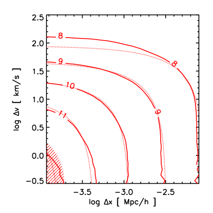
Figure 2: Contours of the logarithm of the particle phase space average density ($P^{2}SAD$) of the Aq-A-2 halo (solid) and for the model described in Section 4 (dotted) at different redshifts, clockwise from top left: $z=0$ (black), $z=0.95$ (red), $z=2.2$ (cyan) and $z=3.5$ (orange). The dashed regions in the left corners encompass the regions where resolution is a potential issue (see Appendix of Paper I).

After $z^{\ast}$, the density does not dilute anymore as the Universe expands. If $z_{\rm inf}>z^{\ast}$ we then have an additional solution to Eq. (20) for $z<z^{\ast}$:

$$\left(\frac{\rho_{\rm sub}(z;r)}{\rho_{\rm sub}(z^{\ast})}\right)^{\alpha} = 1-\alpha A_{\rm tid}\sqrt{75/\pi}\left.\left[\frac{\rho_{\rm host}(<r)}{200\rho_{\rm crit}(z=0)}\right]^{1/2}\right|_{\rm ren}$$ (27)

$$\times \left.\left(\frac{\phi(r)_{,rr}}{4\pi G\rho_{\rm host}(r)}\right)^{\alpha}\right|_{\rm ren}T(z^{\ast},z),$$

where

$$T(z^{\ast},z)=\int_{z}^{z^{\ast}}\frac{\left(\Omega_{m}\left(1+z\right)^{3}+\Omega_{\Lambda}\right)^{-1/2}}{1+z}dz,$$ (28)

and the subscript $ren$ means that the quantity is renormalized to the radius where the average solution applies, i.e., to $r=r_{200}$. If $z_{\rm inf}<z^{\ast}$, then only this “second mode” (Eq.27) of stripping occurs.

In the end, we have a model of tidal disruption with $5$ free parameters: $A_{\rm tid}$, $\alpha$, $f$, $\tilde{B}$ and $\kappa$, in addition to the improved stable clustering prediction which includes $3$ additional free parameters (which in principle could depend on redshift and in halo-centric distance): $a(z,r)$, $b(z,r)$ and $\beta(z,r)$ accounting for the stretching in phase space due to tidal shocking (Eq.19). This model is able to describe the small-scale behaviour of $P^{2}SAD$ at different redshifts and at different regions within the halo as we show in the following section.

5 Simulation data and model comparison

5.1 Average behaviour within the virialized halo and redshift dependence

We first compare the model developed in Section 4 with the value of $P^{2}SAD$ averaged over all particles that are gravitationally bound to the Aq-A-2 halo, i.e., those in the smooth and substructure components (for a more detailed definition see the first paragraphs of section 3 of Paper I). Fig. 2 shows the small scale behaviour of $P^{2}SAD$ in the simulation at different redshifts (solid lines) and fits by our model in dotted lines. Although the fits are poorer for $\Xi>10^{9}{\rm M}_{\odot}h^{2}/({\rm Mpc~{}\rm km/s})^{3}$ (particularly at $z>2$), it is clearly a reasonable description at smaller scales (i.e., separations in phase space), which are the ones that matter the most to extrapolate the behaviour to the unresolved scales.

The variations across redshift can be accommodated by introducing a slight redshift dependence of the parameters $\beta$, $a$ and $b$. The former is given by a simple linear relation as in Paper I:

$$\beta(z)=0.67+0.08(1+z)$$ (29)

while $a(z)$ and $b(z)$ are given in Table 2.

Redshift	$a$	$b$
0.0	$0.29$	$1.77$
0.95	$0.26$	$1.75$
2.2	$0.28$	$1.77$
3.5	$0.24$	$1.77$

Table 2: Values of the fitting parameters in Eq. (19) that together with the tidal disruption model explained in Section 4.1 provide a good description of $P^{2}SAD$ at small $(\Delta x,\Delta v)$ (see Fig. 2).

The full tidal stripping model described in Section 4.1 fits the simulated data with the following values for the five free parameters: $f=2.1$, $\alpha=1/3$, $A_{\rm tid}=0.12$, $\tilde{B}=0.185$ and $\kappa=4.5$. Although we did not explore exhaustively the large parameter space we found that large deviations from these values seem to give a poorer fit (this is especially the case for $f$ and $\alpha$). We also note that the behaviour of $\mu$ as a function of mass and redshift can be roughly approximated by the following formula (up to $z\sim 2$):

$$\mu(z;m_{\rm col})\approx 0.01\left[1+\left(\frac{m_{\rm col}(1+z)^{2.5}}{10^{8}{\rm M}_{\odot}}\right)^{0.22}\right]$$ (30)

5.2 Halo-centric distance dependence

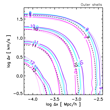
Figure 3: Contours of the logarithm of the particle phase space average density ($P^{2}SAD$) for the Aq-A-2 halo at $z=0$ for samples of particles taken at different radial shells from the halo centre. Left panel: $0<r/r_{200}<0.2$ (red) and $0.2<r/r_{200}<0.4$ (blue). Right panel: $0.4<r/r_{200}<0.6$ (magenta), $0.6<r/r_{200}<0.8$ (cyan), and $0.8<r/r_{200}<1.0$ (violet). The dotted lines are fits given by our model described in section 4. The relevant parameters of the fits are given in Table 3. For reference, the dashed line is $P^{2}SAD$ averaged over the whole halo.

Fig. 3 shows the contours of log($P^{2}SAD$) averaged over particles that are located in concentric shells at different distances from the halo centre as described in the caption. The solid lines are the simulation data for the Aq-A-2 halo while the dashed lines are the result of our model with the same value of the free parameters associated to $\mu$ as in the previous average case (i.e., $f=2.1$, $\alpha=1/3$, $A_{\rm tid}=0.12$, $\tilde{B}=0.185$ and $\kappa=4.5$). We note that $\mu$ is a function of radius through Eq. (27) that can be approximated by:

$$\mu(r;m_{\rm col})\approx\mu_{0}(r)\left[c_{\mu}(r)+\left(\frac{m_{\rm col}}{10^{8}{\rm M}_{\odot}}\right)^{\alpha_{\mu}(r)}\right]$$ (31)

where the radial-dependent parameters $\mu_{0}(r)$, $c_{\mu}(r)$ and $\alpha_{\mu}(r)$, as well as the shape parameters $a$, $b$ and $\beta$, that fit the simulation data are given in Table 3.

$r/r_{200}$	$\beta$	$a$	$b$	$\mu_{0}$	$\alpha_{\mu}$	$c_{\mu}$
0.0-0.2	$1.0$	$0.17$	$1.55$	$0.0045$	$0.15$	$0.15$
0.2-0.4	$0.9$	$0.20$	$1.45$	$0.0135$	$0.13$	$0.20$
0.4-0.6	$0.8$	$0.28$	$1.55$	$0.0160$	$0.12$	$0.25$
0.6-0.8	$0.775$	$0.35$	$1.72$	$0.0160$	$0.12$	$0.25$
0.8-1.0	$0.75$	$0.40$	$1.80$	$0.0160$	$0.12$	$0.25$

Table 3: The second, third and fourth columns are the values of the parameters in Eq. (3) for the fit to $P^{2}SAD$ averaged over different radial shells centered in the Aq-A-2 halo as indicated in the first column (see Fig.3). The last three columns are the parameters of a simple approximation (Eq. 31) of the parameter that controls tidal stripping ($\mu(r;m_{\rm col})$; see Section 4.1).

6 Boost to Dark Matter Annihilation due to unresolved sub-structure

Once we have calibrated the model to the simulation data, we can use it to extrapolate the behaviour of $P^{2}SAD$ to scales that are unresolved. We argue that this extrapolation method offer advantages over other commonly used methods in the computation of the boost to the annihilation rate due to gravitationally bound unresolved substructures. This is the case especially for methods that extrapolate the concentration-mass relation. The support for this argument is two-fold:

• The small scale modelling of $P^{2}SAD$ is physically motivated by: the stable clustering hypothesis in phase space, the spherical collapse model, and a simplified tidal disruption description.

• The structure of $P^{2}SAD$ is directly connected to the annihilation rate (Eq.4), with the small scale behaviour reflecting the substructure contribution.

By calibrating the model to $P^{2}SAD$, we avoid the use of the subhalo model and instead of uncertainties on the abundance of subhaloes, their radial distribution, and their internal properties, our model is sensitive to the behaviour of $\mu(m_{\rm col})$ and to the assumption that all other shape parameters remain unchanged at unresolved scales. However, as we show below, of all these, $b$ is the only one of relevance.

As a first example, let us compute the total annihilation rate due to substructures within a MW-size halo at $z=0$ in the case of $(\sigma_{\rm ann}v)={\rm const}$:

$$R_{\rm ann}^{\rm subs} = \frac{4\pi M_{200}(\sigma_{\rm ann}v)}{2m_{\chi}^{2}}\int(\Delta v)^{2}d\Delta v\lim_{\Delta x\to 0}\Xi^{\rm sub}(\Delta x,\Delta v)=\frac{4\pi M_{200}(\sigma_{\rm ann}v)}{2m_{\chi}^{2}}\int\frac{b^{3}}{2}(F^{-1}(\mu\xi_{s}))^{1/2}\frac{dF^{-1}}{dm_{\rm col}}\mu(m_{\rm col})\xi_{s}(m_{\rm col})dm_{\rm col}$$ (32)

$$= \frac{8\pi^{1/2}b^{3}}{9\delta_{c}^{3}}200\rho_{crit,0}M_{200}\frac{(\sigma_{\rm ann}v)}{2m_{\chi}^{2}}\int_{\rm m_{min}}^{\rm m_{max}}\mu(m_{\rm col})m_{\rm col}^{-2}d(m_{\rm col}^{2}\sigma^{3}(m_{\rm col}))$$

where we have used Eqs.(12),(14),(17), and (19). Notice that only $b$ and $\mu$ enter into the annihilation rate (i.e., $\beta$ and $a$ are irrelevant). The limits of the integral are the minimum and maximum subhalo masses at collapse that contribute to $P^{2}SAD$, which are non-trivially connected to the tidally disrupted subhalo masses today. With the values of $\Xi^{\rm zero}_{\rm min}$ ($\Xi^{\rm zero}_{\rm max}$) mentioned in Section 3 corresponding to resolved subhaloes we can directly estimate $m_{\rm min}\sim 10^{7}$M_⊙ ($m_{\rm max}\sim 10^{11}$M_⊙) since $\Xi=\mu\xi_{s}$. These masses are a factor of several above the minimum (maximum) subhalo masses at $z=0$ contributing to $P^{2}SAD$ in the Aq-A-2 halo.

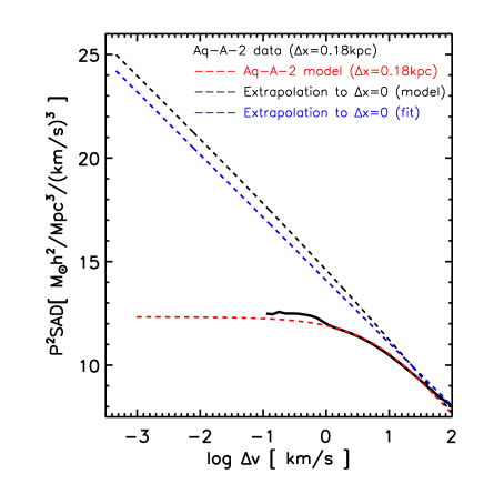
Figure 4: Projection of the particle phase space average density ($P^{2}SAD$) for the Aq-A-2 halo at $z=0$ in the $\Delta v$ direction fixing $\Delta x\sim 0.18$ kpc (black solid). The red dashed line is the fit with our model using the same cut in $\Delta x$, while the black and blue dashed lines are extrapolations to $\Delta x=0$ using our full model and using the fitting function in Eq. (2), respectively. The horizontal axis is extended all the way to the value of $\Delta v$ corresponding to $m_{\rm col}=10^{-6}$M_⊙, the typical mass of WIMP models.

The projection of $P^{2}SAD$ along the $\Delta v$ direction can be seen in Fig. 4 for the whole virialized region of Aq-A-2 at $z=0$. This is the quantity of interest to compute the annihilation rate and we show with a black solid line the case when $\Delta x\sim 0.18$ kpc (which is the minimum physical separation we can resolve). The dashed red line is a fit by our full model with the same cut in $\Delta x$ while the limit to $\Delta x=0$ in the model is shown with a black dashed line. The extrapolation using the fitting function that directly relates $\Delta v$ with $P^{2}SAD$ (see Eq. 2) is shown with a blue dashed line. We have extended the horizontal axis to the corresponding velocity separations of WIMP models with $m_{\rm col}=10^{-6}$M_⊙. From Fig. 4 we can see that the simple formula (see Eq. 2):

$$\lim_{\Delta x\to 0}\Xi^{\rm sub}(\Delta x,\Delta v)=(\Delta v/q_{V})^{3}$$ (33)

provides a good approximation to our full modelling and it immediately suggests that the annihilation rate scales roughly logarithmically with $P^{2}SAD$ (for $\sigma_{\rm ann}v={\rm const}$).

We use Eq. (32) to compute the subhalo boost (using the smooth Einasto distribution described in Section 3) as a function of the minimum collapsed mass down to the decoupling masses corresponding to WIMPs; this is shown in Fig. 5. The filled circle is the value in Eq. (11) corresponding to resolved substructures and found directly with the small scale fitting function of $P^{2}SAD$ in Section 3 (i.e., Eq. 10). The star symbol on the right (left) is shown for reference, and corresponds to the subhalo boost reported by Springel et al. (2008) for a minimum subhalo mass $m_{\rm sub}(z=0)=10^{6}$($10^{-6}$) M_⊙. The extrapolation in this case was done under the assumption that the radial subhalo luminosity profile preserves its shape and that the re-scaling of the normalisation with $m_{\rm sub}(z=0)$ follows the resolved trend. Recall that these are not the masses at collapse so to put the circle and star symbols on the right of Fig. 5 we use $m_{\rm sub}(z=0)\sim 10^{6}$M${}_{\odot}\rightarrow m_{\rm min}\sim 10^{7}$M_⊙ as explained two paragraphs above, while the location of the star symbol on the left of the figure is somewhat uncertain. The triangle symbol is the extrapolation to lower masses made by Kamionkowski et al. (2010) using the probability distribution function of the density field (subhaloes imprint a power-law tail in this PDF) calibrated with the MW-sized simulation Via Lactea II (Diemand et al., 2008). The results from our method are quite close to those found by Kamionkowski et al. (2010) and are an order of magnitude lower than the estimates by Springel et al. (2008).

Zavala et al. (2010) also estimated a subhalo boost with a statistical analysis of all haloes in the Millennium-II simulation (Boylan-Kolchin et al., 2009), implicitly extrapolating the subhalo mass function and concentration-mass relation to the unresolved regime. They found a large range of possible subhalo boosts, within $2-2\times 10^{3}$, depending on the exact parameters of the extrapolation, for a $\sim 10^{12}$M_⊙ halo.

Figure 5: Total subhalo boost to the annihilation rate (assuming $(\sigma_{\rm ann}v)={\rm const}$) within the virialized region of a MW-size halo as a function of the minimum subhalo mass at collapse. The filled circle shows the value of the boost estimated directly from the fit to the simulation data (Eq. 11), while the star symbols are the values in the resolved ($m_{\rm sub}(z=0)\geq 10^{6}$M_⊙) and extrapolated cases ($m_{\rm sub}(z=0)\geq 10^{-6}$M_⊙) taken from Springel et al. (2008). The filled triangle is the boost estimated by Kamionkowski et al. (2010) using a method calibrated with the Via Lactea II simulation (Diemand et al., 2008). The dotted region shows the theoretical expectation for the decoupling mass limit of WIMPs (Bringmann, 2009).

6.1 Sommerfeld-enhanced models

If the annihilation cross-section is enhanced by a Sommerfeld mechanism (e.g. Arkani-Hamed et al., 2009; Pospelov & Ritz, 2009), then the annihilation rate increases with lower relative velocities until saturating due to the finite range of the interaction between the particles prior to annihilation. Instead of using a specific Sommerfeld-enhanced model, we generically approximate the cross section as:

$$(\sigma_{\rm ann}v) = (\Delta v/c)^{-\beta_{\rm S}}(\sigma_{\rm ann}v)_{0},\ \ \ \ \ \Delta v>\Delta v_{\rm sat}$$

$$(\sigma_{\rm ann}v) = S_{\rm sat}(\sigma_{\rm ann}v)_{0},\ \ \ \ \ \Delta v\leq\Delta v_{\rm sat}$$ (34)

The value of $\beta_{\rm S}$ is commonly near $1$ (the so-called “$1/v$” boost), but it can reach $2$ near resonances; we only consider the former case. For Eq. (6.1) and using our modelling we obtain:

$$R_{\rm ann}^{\rm subs}(SE) = \frac{8\pi^{1/2}b^{3}}{9\delta_{c}^{3}}200\rho_{crit,0}M_{200}\frac{(\sigma_{\rm ann}v)_{0}}{2m_{\chi}^{2}}\times\Bigg{[}S_{\rm sat}\int_{\rm m_{min}}^{\rm m_{sat}}\mu(m_{\rm col})m_{\rm col}^{-2}d(m_{\rm col}^{2}\sigma^{3}(m_{\rm col}))$$ (35)

$$+ \left(\frac{\left(10H_{0}G\right)^{2/3}}{\pi\delta_{c}c^{2}}\right)^{-\beta_{\rm S}/2}\int_{\rm m_{sat}}^{\rm m_{max}}\left(m_{\rm col}^{2/3}\sigma(m_{\rm col})\right)^{-\beta_{\rm S}/2}\mu(m_{\rm col})m_{\rm col}^{-2}d(m_{\rm col}^{2}\sigma^{3}(m_{\rm col}))\Bigg{]}$$

where $m_{\rm sat}$ is the collapse mass corresponding to the characteristic velocity at saturation $\Delta v_{\rm sat}$; using Eq. (19):

$$\Delta v_{\rm sat}=b\left(10H_{0}Gm_{\rm sat}\right)^{1/3}\left(\frac{\sigma(m_{\rm sat})}{\pi\delta_{c}}\right)^{1/2}.$$ (36)

Figure 6: Same as Fig. 5 but for a Sommerfeld-like model where $(\sigma_{\rm ann}v)=(\Delta v/c)^{-\beta_{\rm S}}(\sigma_{\rm ann}v)_{0}$ with $\beta_{\rm S}=1.0$ and different saturation values as shown in the legend. The dotted line is an approximation to one of the benchmark points (BM1) presented in Finkbeiner et al. (2011) that avoid different astrophysical constraints and can account for high energy cosmic ray excesses.The dotted region shows the theoretical expectation for the decoupling mass limit of WIMPs (Bringmann, 2009).

Fig. 6 shows the subhalo boost, relative to the smooth dark matter distribution of the host halo, for Sommerfeld-like models where the cross section scales as in Eq. (6.1) with $\beta_{\rm S}=1$. To compute the Sommerfeld-enhanced smooth component, we simply took the annihilation rate corresponding to the Einasto profile, defined in Section 3, and scaled it up based on the characteristic velocity dispersion of the Aq-A-2 halo: $R_{\rm ann}^{\rm smooth}(SE)=S(\sigma_{\rm disp}^{\rm host})R_{\rm ann}^{\rm smooth}$, with $\sigma_{\rm disp}^{\rm host}\sim 120{\rm kms}^{-1}$. The solid line is for $S_{\rm sat}=2500\sim S(\sigma_{\rm disp}^{\rm host})$; below this value, all substructures are saturated and thus the boost is just a trivial scaled version of that shown in Fig. 5. The dotted line roughly approximates one of the benchmark point models defined in Finkbeiner et al. (2011) (BM1 in their Table 1) to satisfy a number of astrophysical constraints (relic abundance, CMB power spectrum, etc.) while at the same time providing a fit to the cosmic ray excesses observed by the PAMELA and Fermi satellites. Enhancements much larger than this value (e.g. dashed line, $S_{\rm sat}=20000$) are likely ruled out by astrophysical constraints but illustrate the transition between the unsaturated and saturated regimes. We note that BM1 is still compatible with the new measurement of the positron excess reported by the AMS collaboration (see Cholis & Hooper, 2013). Since allowed Sommerfeld-enhanced models in the parameterisation we have used have $S_{\rm sat}\gtrsim S_{\rm host}$, then the enhanced substructure boost is at the end just a scaled version of the constant cross section boost: ${\rm Boost(SE)}\sim S_{\rm sat}/S_{\rm host}\times{\rm Boost(\sigma_{\rm ann}v=const)}$.

6.2 Halo-centric distance boost

Finally, we can also apply our methodology to compute the substructure boost as a function of the distance to the halo centre. To do so, all that is needed is to replace the global values of the parameters $b$ and $\mu(m_{\rm col})$ for the radial dependent values that we fit to the simulation data in Section 5, and to account for the renormalisation in mass of the phase-space volume where $P^{2}SAD$ is averaged. A simple but good approximation for $\mu(r;m_{\rm col})$ is given in Eq. (31). Using it, our results can be easily reproduced with the values given in Table 3.

Figure 7: Subhalo boost to the annihilation rate as a function of halo-centric distance for a minimum subhalo mass at collapse of $10^{-6}$M_⊙. The boost was computed for concentric shells with a thickness of $0.2~{}R_{200}$ in the cases of constant cross section (circle symbols) and for an approximation of the Sommerfeld-enhanced model BM1 presented in Finkbeiner et al. (2011) (star symbols).

Fig. 7 shows the substructure boost to the annihilation rate of the smooth halo as a function of the distance to the halo centre. Since in Section 5.2 we calibrated our fitting parameters in concentric shells with a thickness of $0.2~{}R_{200}$, we plot the results with bars showing the extent of the shells in which $P^{2}SAD$ was averaged. We remark that in this case $M_{{\cal V}_{6}}$ is the total mass in a given shell, not $M_{200}$ as it has been so far in this section. In Fig. 7 we show the cases with $(\sigma_{\rm ann}v)={\rm const}$ (circles) and Sommerfeld-like enhancement corresponding to the benchmark point BM1 (stars) presented in Finkbeiner et al. (2011) (see Section 6.1). Our results are in good agreement with those of Kamionkowski et al. (2010) (see their Fig. 4), although we seem to predict lower boosts in the central regions.

Values specific to a certain radius can be approximated by interpolating $b(r)$ and $\mu(r;m_{\rm col})$ and considering that for small volumes one has $R_{\rm ann}^{\rm smooth}(r)\propto\rho_{\rm smooth}(r)M_{{\cal V}_{6}}$ and thus the subhalo boost can be computed independently of the specific value of $M_{{\cal V}_{6}}$. For instance, for $r=8$ kpc, we find that the boost is only $\sim 0.1\%$ for the constant cross section case, and $\sim 0.2\%$ for the Sommerfeld-like model BM1.

7 Summary and Conclusions

The clustering of dark matter at scales unresolved by current numerical simulations is a key ingredient in many predictions of non-gravitational (and some gravitational) signatures of dark matter. The characteristic scale of the smallest haloes (commonly called microhaloes) contributing to these signals is $\mathcal{O}(10^{-9})$ times the size of the Milky Way halo, and we therefore refer to it as the nanostructure of dark matter haloes. The degree of uncertainty of this nanostructure clustering can be as much as two orders of magnitude for WIMP dark matter models, since the minimum bound haloes have masses $\gtrsim 9$ orders of magnitude below the highest resolution simulations to date. In the case of dark matter annihilation for example, the small, cold and dense dark structures have the dominant contribution to the hypothetical extragalactic signals, and thus the bulk of the predicted annihilation rate comes from extrapolating, in diverse ways, the dark matter clustering from the resolved to the unresolved regime.

Most extrapolation methods rely on assumptions about the abundance, spatial distribution, and internal properties of (sub)haloes. For example, the total subhalo boost to the annihilation rate over the smooth dark matter distribution of a single halo, is typically computed by extrapolating, either explicitly or implicitly, the subhalo mass function and the concentration-mass relation. Extending these functions as power-laws down to lower masses yields the higher boosts. In this paper, we present an alternative method based on a novel perspective on the clustering of dark matter introduced in Zavala & Afshordi (2013) (Paper I). The method rests upon writing the dark matter annihilation rate in a given volume as an integral over velocities of a new coarse-grained Particle Phase Space Average Density ($P^{2}SAD$; see Eqs. 1 and 4).

The structure of $P^{2}SAD$ was analysed in detail in Paper I, where it was found to be nearly universal in time and across different ambient densities, in the regime dominated by substructures. Here we present a model of the structure of $P^{2}SAD$ inspired by the stable clustering hypothesis and the spherical collapse model, and improved by incorporating a prescription for the tidal disruption of subhaloes.

Our modelling provides a physically-motivated explanation of the two-dimensional functional shape of $P^{2}SAD$, and calibrated to the MW-size Aquarius simulations, gives a firm basis to extrapolate into the unresolved substructure regime. In summary, the main advantages of our method are two-fold:

• The free parameters in our model are fitted to a single 2D function that is a very sensitive measure of cold small scale substructure and is directly connected to the annihilation rate.

• The annihilation rate is written as an integral over relative velocities of the “zero-separation” limit of $P^{2}SAD$ multiplied by the annihilation cross section times the relative velocity (see Eq. 4). This allows us to accommodate any velocity-dependence coming from particle physics models in a straightforward way.

Although our model has several free functions that are fitted to the MW-size Aquarius simulations, only two are of relevance for the prediction of the annihilation rate: (i) $b$ in Eq. (19) parametrizes the ratio of phase space volume in spherical collapse, to the characteristic phase space volume of subhaloes at the time of formation; and (ii) $\mu$ in Eq. (12) that can be interpreted as the dilution of the characteristic phase space density at collapse due to tidal disruption. For the simulated data we analised, the former is $\sim 1.8$ and we present tabulated fitted values across redshifts and distances to the MW-halo centre (Tables 2 and 3), while for the latter we present simple parameterisations (see Tables 2 and 3, Eqs. 29-30).

As a sample application of our model, we computed the subhalo boost (over the smooth dark matter distribution) in a MW-size halo, both globally (i.e. over the whole virialized halo) and locally as a function of halo-centric distance, for cases where the annihilation cross section is constant and for a generic Sommerfeld-like enhanced case where $(\sigma_{\rm ann}v)\propto 1/\Delta v$ up to a maximum saturation value. We find that in the former, the global boost is $\sim 15$ for typical WIMP models (with decoupling masses in the range $10^{-11}-10^{-3}$M_⊙).

Our estimate of the subhalo boost is in the low end of current estimates being in agreement with Kamionkowski et al. (2010) (based on a different simulation), and a factor of $\sim 10$ lower than the boost computed in Springel et al. (2008) (based on the same simulation suite than the one used here). The discrepancy with the latter is likely caused by their implicit extrapolation of the subhalo mass function and, perhaps more importantly, the concentration-mass relation. Evidence of this can be seen in the structure of $P^{2}SAD$ in the resolved regime (without recurring to the modelling of the unresolved regime) where our analysis indicates that the annihilation rate (in the $(\sigma_{\rm ann}v)={\rm const}$ case) from substructures scales logarithmically with the maximum (coarse-grained) phase space density (Eq. 10) rather than as a power law. Since we argue that $P^{2}SAD$ is a more direct measure of the annihilation signal, our results seem to disfavour large boost factors.

$P^{2}SAD$ has also other potential applications in dark matter direct detection, pulsar timing and transient weak lensing (see Rahvar et al., 2013) that will be explored in the future.

We have made our code to compute $P^{2}SAD$ (with our full model) publicly available online at http://spaces.perimeterinstitute.ca/p2sad/. Interested users should refer to that site for instructions on how to use the code.

References

- Abazajian et al. (2012) Abazajian K. N., Blanchet S., Harding J. P., 2012, Phys. Rev. D, 85, 043509
- Abdo et al. (2009) Abdo A. A., et al., 2009, Physical Review Letters, 102, 181101
- Ackermann et al. (2011) Ackermann M., et al., 2011, Physical Review Letters, 107, 241302
- Ackermann et al. (2012) Ackermann M., et al., 2012, ApJ, 747, 121
- Adriani et al. (2009) Adriani O., et al., 2009, Nature, 458, 607
- Afshordi & Cen (2002) Afshordi N., Cen R., 2002, ApJ, 564, 669
- Afshordi et al. (2010) Afshordi N., Mohayaee R., Bertschinger E., 2010, Phys. Rev. D, 81, 101301
- Aguilar et al. (2013) Aguilar M., et al., 2013, Physical Review Letters, 110, 141102
- Aprile et al. (2012) Aprile E., et al., 2012, Physical Review Letters, 109, 181301
- Arkani-Hamed et al. (2009) Arkani-Hamed N., Finkbeiner D. P., Slatyer T. R., Weiner N., 2009, Phys. Rev. D, 79, 015014
- Bergström et al. (2009) Bergström L., Edsjö J., Zaharijas G., 2009, Physical Review Letters, 103, 031103
- Boylan-Kolchin et al. (2009) Boylan-Kolchin M., Springel V., White S. D. M., Jenkins A., Lemson G., 2009, MNRAS, 398, 1150
- Bringmann (2009) Bringmann T., 2009, New Journal of Physics, 11, 105027
- Carroll et al. (1992) Carroll S. M., Press W. H., Turner E. L., 1992, ARA&A, 30, 499
- Cholis & Hooper (2013) Cholis I., Hooper D., 2013, Phys. Rev. D, 88, 023013
- Davis & Peebles (1977) Davis M., Peebles P. J. E., 1977, ApJS, 34, 425
- Diemand et al. (2008) Diemand J., Kuhlen M., Madau P., Zemp M., Moore B., Potter D., Stadel J., 2008, Nature, 454, 735
- Finkbeiner et al. (2011) Finkbeiner D. P., Goodenough L., Slatyer T. R., Vogelsberger M., Weiner N., 2011, Journal of Cosmology and Astroparticle Physics, 5, 2
- Fornasa et al. (2013) Fornasa M., Zavala J., Sánchez-Conde M. A., Siegal-Gaskins J. M., Delahaye T., Prada F., Vogelsberger M., Zandanel F., Frenk C. S., 2013, MNRAS, 429, 1529
- Gao et al. (2012) Gao L., Frenk C. S., Jenkins A., Springel V., White S. D. M., 2012, MNRAS, 419, 1721
- Hooper & Slatyer (2013) Hooper D., Slatyer T. R., 2013, arXiv:1302.6589
- Jing (2001) Jing Y. P., 2001, ApJ, 550, L125
- Kamionkowski et al. (2010) Kamionkowski M., Koushiappas S. M., Kuhlen M., 2010, Phys. Rev. D, 81, 043532
- Kuhlen et al. (2008) Kuhlen M., Diemand J., Madau P., 2008, ApJ, 686, 262
- Linden & Profumo (2013) Linden T., Profumo S., 2013, ApJ, 772, 18
- Navarro et al. (2010) Navarro J. F., Ludlow A., Springel V., Wang J., Vogelsberger M., White S. D. M., Jenkins A., Frenk C. S., Helmi A., 2010, MNRAS, 402, 21
- Pospelov & Ritz (2009) Pospelov M., Ritz A., 2009, Physics Letters B, 671, 391
- Rahvar et al. (2013) Rahvar S., Baghram S., Afshordi N., 2013, arXiv:1310.5412
- Siegal-Gaskins (2008) Siegal-Gaskins J. M., 2008, JCAP, 10, 40
- Slatyer et al. (2012) Slatyer T. R., Toro N., Weiner N., 2012, Phys. Rev. D, 86, 083534
- Springel et al. (2008) Springel V., Wang J., Vogelsberger M., Ludlow A., Jenkins A., Helmi A., Navarro J. F., Frenk C. S., White S. D. M., 2008, MNRAS, 391, 1685
- Springel et al. (2008) Springel V., White S. D. M., Frenk C. S., Navarro J. F., Jenkins A., Vogelsberger M., Wang J., Ludlow A., Helmi A., 2008, Nature, 456, 73
- Stadel et al. (2009) Stadel J., Potter D., Moore B., Diemand J., Madau P., Zemp M., Kuhlen M., Quilis V., 2009, MNRAS, 398, L21
- Taruya & Suto (2000) Taruya A., Suto Y., 2000, ApJ, 542, 559
- Vogelsberger et al. (2009) Vogelsberger M., Helmi A., Springel V., White S. D. M., Wang J., Frenk C. S., Jenkins A., Ludlow A., Navarro J. F., 2009, MNRAS, 395, 797
- Zavala & Afshordi (2013) Zavala J., Afshordi N., 2013, arXiv:1308.1098
- Zavala et al. (2010) Zavala J., Springel V., Boylan-Kolchin M., 2010, MNRAS, 405, 593
- Zavala et al. (2011) Zavala J., Vogelsberger M., Slatyer T. R., Loeb A., Springel V., 2011, Phys. Rev. D, 83, 123513