On a cross-diffusion segregation problem arising from a model of interacting particles

Abstract

We prove the existence of solutions of a cross-diffusion parabolic population problem. The system of partial differential equations is deduced as the limit equations satisfied by the densities corresponding to an interacting particles system modeled by stochastic differential equations. According to the values of the diffusion parameters related to the intra and inter-population repulsion intensities, the system may be classified in terms of an associated matrix. For proving the existence of solutions when the matrix is positive definite, we use a fully discrete finite element approximation in a general functional setting. If the matrix is only positive semi-definite, we use a regularization technique based on a related cross-diffusion model under more restrictive functional assumptions. We provide some numerical experiments demonstrating the weak and strong segregation effects corresponding to both types of matrices.

1 Introduction

The effects of spatial cross-diffusion on interacting population models have been widely studied since Kerner [32] and Jorné [31] examined the linear cross-diffusion model

$${\partial_{t}}u_{i}-a_{i1}\Delta u_{1}-a_{i2}\Delta u_{2}=(-1)^{i+1}u_{i}(\alpha_{i}-\beta_{i}u_{j}),$$

with non-negative self-diffusivities $a_{ii}$, and non-zero cross-diffusivities $a_{ij}$, for $i,j=1,2,~{}i\neq j$, and demonstrated that while self-diffusion tends to damp out all spatial variations in the Lotka-Volterra system, cross-diffusion may give rise to instabilities [42] and to non-constant stationary solutions.

First nonlinear cross-diffusion models seem to have been introduced by Busenberg and Travis [10] (see also Gurtin and Pipkin [30] for a related model), and Shigesada et al. [45] from different modeling points of view. Shigesada et al. approach starts with the assumption of a single population density evolution determined by a continuity equation

$${\partial_{t}}u-\operatorname{div}J(u)=u(\alpha-\beta u),\quad\text{with }J(u)=\nabla((c+au)u)+bu\nabla\Phi.$$ (1)

The divergence of the flow $J$ is thus decomposed into three terms: a random dispersal, $c\Delta u$, a dispersal caused by population pressure, $a\Delta u^{2}$, and a drift directed to the minima of the environmental potential $\Phi$. Generalizing this scalar equation to two populations they propose the system, for $i=1,2$,

$${\partial_{t}}u_{i}-\operatorname{div}J_{i}(u_{1},u_{2})=f_{i}(u_{1},u_{2}),$$

with

$$J_{i}(u_{1},u_{2})=\nabla\big{(}(c_{i}+a_{i1}u_{1}+a_{i2}u_{2})u_{i}\big{)}+b_{i}u_{i}\nabla\Phi,$$ (2)

and $f_{i}$ of the competitive Lotka-Volterra type. Disregarding the linear dispersals ($c=c_{i}=0$) representing a random contribution to the motion, the nonlinear part of the flow $J$ in Eq. 1 may be expressed in conservative form as $J(u)=u\tilde{J}(u)$, with $\tilde{J}$ given by the potential $\tilde{J}(u)=\nabla(2au+b\Phi)$. However, rewriting the flows (2) in a similar way leads to the more intricate expression

$$\tilde{J}_{i}(u_{1},u_{2})=\big{(}2a_{ii}u_{i}+a_{ij}\frac{u_{j}}{u_{i}}\big{)}\nabla u_{i}+a_{ij}\nabla u_{j}+b_{i}\nabla\Phi,$$

which, in general, can not be deduced from a potential. This fact has been one of the main difficulties in finding appropriate conditions ensuring the existence of solutions to the model proposed by Shigesada et al. (SKT model, from now on), see [33, 18, 54, 38, 21, 22, 13, 4, 52, 20] and their references.

The generalization of the flow in (1) to several populations (with $c=b=0$) given by Busenberg and Travis [10] is perhaps more natural from the modeling point of view. They assume that the individual population flow $J_{i}$ is proportional to the gradient of a potential function, $\Psi$, that only depends on the total population density $U=u_{1}+u_{2}$,

$$J_{i}(u_{1},u_{2})=a\frac{u_{i}}{U}\nabla\Psi(U).$$

Note that in this way the flow of $U$ is still given in the form (1), with $J(U)=a\nabla\Psi(U)$ (and $c=b=0$). Assuming the power law $\Psi(s)=s^{2}/2$, we obtain individual population flows given by

$$J_{i}(u_{1},u_{2})=au_{i}\nabla U,$$ (3)

as those introduced by Gurtin and Pipkin [30] and mathematically analyzed by Bertsch et al. [7, 9].

In this article we propose a generalization of the Busenberg-Gurtin model consisting on the assumption that the individual flows $J_{i}$ depend, instead of in the total population density $u_{1}+u_{2}$, in a general linear combination of both population densities, possibly different for each population. As remarked in [30], these weighted sums are motivated when considering a set of species with different characteristics, such as size, behavior with respect to overcrowding, etc. In addition, we also assume that the flows may contain environmental and random effects, which altogether lead to the following form

$$J_{i}(u_{1},u_{2})=u_{i}\nabla(a_{i1}u_{1}+a_{i2}u_{2}+b_{i}\Phi)+c_{i}\nabla u_{i},$$

which (for $c_{i}=0$) has a conservative form similar to that of the scalar case. We shall refer to this model as the BT model.

Let us finally remark that cross-diffusion parabolic systems have been used to model a variety of phenomena ranging from ecology [28, 50, 24, 20, 44, 1], to semiconductor theory [14, 16], granular materials [3, 23, 39] or turbulent transport in plasmas [17], among others. Apart from global existence and regularity results for the evolution problem, construction of traveling wave solutions [53] or exact solutions [15] have been accomplished. For the steady state problem, existence of non constant steady state solutions has been proven in [37, 38]. Other interesting properties, such as pattern formation, has been studied in [51, 26, 43, 27]. Finally, the numerical discretization has received much attention, and several schemes have been proposed [21, 22, 4, 25, 2, 6].

The article is organized as follows. In Section 2, for a better physical understanding of our model, we sketch a heuristic deduction based on stochastic dynamics of particle systems. In Section 3 we give the precise assumptions on the data problem and state the main results. In Section 4, we introduce the approximated problems and perform some numerical experiments showing the behavior of solutions under several choices of the parameters, including a comparison between the SKT and the BT models. In Section 5, we prove the theorems stated in Section 3 , finally, in Section 6 we present our conclusions.

2 Mathematical modeling

In recent years there has been a trend to the rigorous deduction of Eq. (1) as the equation satisfied by the limit density distribution of suitable particle stochastic systems of differential equations, see [40, 41, 49, 34] and their references. We sketch here the formulation and the main ideas contained in these works which allow us to deduce our model.

Consider a system of $N=N_{1}+N_{2}$ interacting particles of two different types described by their trajectories $X^{i}_{j_{i}}:\mathbb{R}_{+}\to\mathbb{R}^{m}$, $j_{i}=1,\ldots,N_{i}$, $i=1,2$ (stochastic processes). We take $N_{1}=N_{2}=n$ to simplify the notation. The Lagrangian approach to the description of the system is based on specifying suitable interacting laws among particles in such a way that their trajectories are determined by solving the following stochastic system of ordinary differential equations (SDE)

$$dX^{i}_{j}(t)=F^{i}_{j}(X^{1}_{1}(t),\ldots,X^{1}_{n}(t),X^{2}_{1}(t),\ldots,X^{2}_{n}(t))dt+\sigma^{i}_{n}dW^{i}_{j}(t),$$ (4)

together with some initialization of the processes $X^{i}_{j}(0)=X^{i}_{j0}$, $j=1,\ldots,n$, $i=1,2$. Functions $F_{j}^{i}:\mathbb{R}^{2n}\to\mathbb{R}^{m}$ describe deterministic interactions among particles while the constants $\sigma^{i}_{N}$ are the intensities of random dispersal, due to a variety of factors, described by the Brownian motions $W^{i}_{j}$, with $\left\{W^{i}_{1},\ldots,W^{i}_{n}\right\}$, $i=1,2$, two families of independent standard Wiener processes valued in $\mathbb{R}^{m}$.

The individual particles state may be modeled as positive Radon measures

$$\epsilon_{X^{i}_{j}(t)}(B)=\left\{\begin{array}[]{ll}1&\text{if }X^{i}_{j}(t)\in B\\ 0&\text{if }X^{i}_{j}(t)\notin B\end{array}\right.\quad\text{for all }B\in{\mathcal{B}}(\mathbb{R}^{m}),$$

where ${\mathcal{B}}(\mathbb{R}^{m})$ denotes the Borel $\sigma-$algebra generated by open sets in $\mathbb{R}^{m}$, while the collective behavior of the discrete system may be given in terms of the spatial distribution of particles at time $t$, expressed through the empirical measures

$$u^{i}_{n}(t)=\frac{1}{n}\sum_{j=1}^{n}\epsilon_{X^{i}_{j}(t)}\in{\mathcal{M}}(\mathbb{R}^{m}),$$ (5)

which give the spatial relative frequency of particles of the $i$-th population, at time $t$. Introducing, for $\varepsilon>0$, a regularization-scaling kernel $\zeta_{\varepsilon}(\cdot)=\varepsilon^{-m}\zeta(\cdot/\varepsilon)$, with $\zeta\in C_{0}^{\infty}(\mathbb{R}^{m})$, $\zeta\geq 0$ and $\int\zeta=1$, we may assume that the force exerted on the $j$-th single particle of the $i$-th population located at $X^{i}_{j}(t)$ due to the interaction with all the other particles is given by

$$I^{i}_{j}=\sum_{k=1}^{2}\frac{a_{ik}}{n}\sum_{l=1}^{n}\zeta_{\varepsilon}(X^{i}_{j}(t)-X^{k}_{l}(t)),$$

which may be expressed, using the convolution product, as

$$I^{i}_{j}=\sum_{k=1}^{2}a_{ik}(u^{k}_{n}(t)*\zeta_{\varepsilon})(X^{i}_{j}(t)).$$

Here, the non-negative coefficients $a_{ik}$ represent the repulsion, pressure or compression intensity of inter- and intra-specific types, while parameter $\varepsilon$ determines the type of interaction: macro, micro or mesoscale, see [40]. The Lagrangian description of the dynamics of our system of interacting particles (4) may be rewritten in terms of the empirical measures as

$$dX^{i}_{j}(t)=F^{i}[u^{1}_{n}(t),u^{2}_{n}(t)](X^{i}_{j}(t))dt+\sigma^{i}_{n}dW^{i}_{j}(t),\quad j=1,\ldots,n.$$ (6)

We distinguish two kinds of deterministic interactions assuming $F^{i}=F^{i}_{1}+F^{i}_{2}$, with $F^{i}_{1}$ a repulsive interaction between particles given as

$$F^{i}_{1}[u^{1}_{n}(t),u^{2}_{n}(t)](X^{i}_{j}(t))=-\nabla I_{j}^{i}=-\sum_{k=1}^{2}a_{ik}(u^{k}_{n}(t)*\nabla\zeta_{\varepsilon})(X^{i}_{j}(t)),$$

and $F_{2}$ a local force, independent of the scaling parameter, derived from a potential $\Phi:\mathbb{R}^{m}\to\mathbb{R}$

$$F_{2}[u^{1}_{n}(t),u^{2}_{n}(t)](X^{i}_{j}(t))=b_{i}\nabla\Phi(X^{i}_{j}(t)),$$

with $b_{i}\in\mathbb{R}$. Finally, with respect to the stochastic part of system (6), we assume

$$\lim_{n\to\infty}\sigma^{i}_{n}=\sigma_{i}\geq 0.$$

Observe that, in some contexts, $\sigma^{i}_{n}$ stands for the mean free path, i.e., the average distance covered by a moving particle between successive collisions. Therefore, the sequence $\sigma^{i}_{n}>0$ should be decreasing with respect to $n$, and a vanishing limit $\sigma_{i}$ must not be discarded.

2.1 The Euler description

A fundamental tool in the derivation of the Eulerian model corresponding to the Lagrangian description (6) is Ito’s formula for the time evolution of any smooth scalar function $f(X^{i}_{j}(t),t)$. Introducing the notation

$$\left\langle\mu,g\right\rangle=\int g(s)\,d\mu(s),$$

for the duality ${\mathcal{M}}(\mathbb{R}^{m})\times\mathcal{C}_{0}(\mathbb{R}^{m})$, we deduce for $i=1,2$

$$\left\langle u^{i}_{n}(t),f(\cdot,t)\right\rangle= \frac{1}{n}\sum_{j=1}^{n}f(X_{j}^{i}(t),t)=\left\langle u^{i}_{n}(0),f(\cdot,0)\right\rangle$$

$$-\sum_{k=1}^{2}a_{ik}\int_{0}^{t}\left\langle u^{i}_{n}(s),(u^{k}_{n}(s)*\nabla\zeta_{\varepsilon})(\cdot)\nabla f(\cdot,s)\right\rangle ds$$

$$+b_{i}\int_{0}^{t}\left\langle u^{i}_{n}(s),\nabla\Phi\cdot\nabla f(\cdot,s)\right\rangle ds$$

$$+\int_{0}^{t}\left\langle u^{i}_{n}(s),\frac{\partial}{\partial s}f(\cdot,s)+\frac{1}{2}(\sigma^{i}_{n})^{2}\Delta f(\cdot,s)\right\rangle ds$$

$$+\frac{\sigma^{i}_{n}}{n}\sum_{j=1}^{n}\int_{0}^{t}\nabla f(X^{i}_{j}(s),s)\cdot dW^{i}_{j}(s).$$

The last term of this identity

$$M^{i}_{n}(f,t)=\frac{\sigma_{n}^{i}}{n}\sum_{j=1}^{n}\int_{0}^{t}\nabla f(X^{i}_{j}(s),s)\cdot dW^{i}_{j}(s)$$

is the only explicit source of stochasticity in the equation and shows how, when the number of particles $n$ is large but still finite, also from the Eulerian point of view the system keeps the stochasticity which characterizes each individual. However, Doob’s inequality [19] implies that $M^{i}_{n}(f,t)\to 0$ as $n\to\infty$ in probability, for any $f\in L^{\infty}(0,T;W^{1,\infty}(\mathbb{R}^{m}))$. In other words, the Eulerian description becomes deterministic when the size of the particle system tends to infinity.

Now assume that $u^{i}_{n}(t)$ tends, as $n\to\infty$, to a deterministic process $u^{i}_{\infty}(t)$ which may be represented by a density function $u_{i}$ with respect to the Lebesgue measure on $\mathbb{R}^{m}$ so that, for any $t>0$

$$\lim_{n\to\infty}\left\langle u^{i}_{n}(t),f(\cdot,t)\right\rangle=\left\langle u^{i}_{\infty}(t),f(\cdot,t)\right\rangle=\int_{\mathbb{R}^{m}}f(x,t)u_{i}(x,t)dx.$$

Then, in the limit $n\to\infty$ we formally obtain from (2.1) (see [11, 34] for the rigorous deduction of this limit)

$$\int_{\mathbb{R}^{m}}f(x,t)u_{i}(x,t)dx= \int_{\mathbb{R}^{m}}f(x,0)u_{i}(x,0)dx$$

$$-\sum_{k=1}^{2}a_{ik}\int_{0}^{t}\int_{\mathbb{R}^{m}}u_{i}(x,s)\nabla u_{k}(x,s)\cdot\nabla f(x,s)dxds$$

$$+b_{i}\int_{0}^{t}\int_{\mathbb{R}^{m}}u_{i}(x,s)\nabla\Phi(x)\cdot\nabla f(x,s)dxds$$

$$+\int_{0}^{t}\int_{\mathbb{R}^{m}}u_{i}(x,s)\big{(}\frac{\partial}{\partial s}f(x,s)+\frac{1}{2}\sigma_{i}^{2}\Delta f(x,s)\big{)}dxds,$$

which may be recognized as a weak formulation of the following Cauchy PDE problem for the unknowns $u_{i}:\mathbb{R}^{m}\times\mathbb{R}_{+}\to[0,1]$

$${\partial_{t}}u_{i}-\operatorname{div}\big{(}u_{i}(a_{i1}\nabla u_{1}+a_{i2}\nabla u_{2}-b_{i}\nabla\Phi)\big{)}-c_{i}\Delta u_{i}=0\quad\text{in }\mathbb{R}^{m}\times\mathbb{R}_{+},$$ (8)

for initial data $u_{i}(\cdot,0)=u_{i0}$ in $\mathbb{R}^{m}$, and $c_{i}=\sigma_{i}^{2}/2$.

Let us, finally, remark that the deduction of the Cauchy problem (8) is not easily extended to boundary value problems. In which respects to the non-flow boundary conditions studied in the next section, the corresponding SDE system seem to be the so-called Skorohod or reflecting boundary (stochastic) problem, in which particles are reflected in some prescribed direction when hitting the boundary. Although there exists an abundant literature on this problem, see for instance [36, 48, 47] and their references, to the knowledge of the authors there is not a rigorous deduction of a PDE problem satisfied by the corresponding limit density.

3 Assumptions and main results

Inspired by the problem deduced in the previous section, we set the following one: Given a fixed $T>0$ and a bounded set $\Omega\subset\mathbb{R}^{m}$, find $u_{i}:\Omega\times(0,T)\to\mathbb{R}$ such that, for $i=1,2$,

$${\partial_{t}}u_{i}-\operatorname{div}J_{i}(u_{1},u_{2})=f_{i}(u_{1},u_{2}) \quad\text{in }Q_{T}=\Omega\times(0,T),$$ (9)

$$J_{i}(u_{1},u_{2})\cdot n=0 \quad\text{on }\Gamma_{T}=\partial\Omega\times(0,T),$$ (10)

$$u_{i}(\cdot,0)=u_{i0} \quad\text{in }\Omega,$$ (11)

with flow and competitive Lotka-Volterra functions given by

$$J_{i}(u_{1},u_{2})=u_{i}\big{(}a_{i1}\nabla u_{1}+a_{i2}\nabla u_{2}+b_{i}q\big{)}+c_{i}\nabla u_{i},$$ (12)

$$f_{i}(u_{1},u_{2})=u_{i}\big{(}\alpha_{i}-\beta_{i1}u_{1}-\beta_{i2}u_{2}\big{)},$$ (13)

where the coefficients $a_{ij},~{}c_{i},~{}b_{i},~{}\alpha_{i},~{}\beta_{ij}$, $i,j=1,2$ are assumed to be functions, and not merely constants. Observe that we also replaced the potential field $\nabla\Phi$ of the model derived in the previous section by a general field $q$. We make the following hypothesis on the data, which we shall refer to as (H):

1. $\Omega\subset\mathbb{R}^{m}$ ($m=1,2$ or $3$) is a bounded set with Lipschitz continuous boundary $\partial\Omega$.

2. For $i,j=1,2$, the coefficients $a_{ij},~{}c_{i},~{}\alpha_{i},~{}\beta_{ij}\in L^{\infty}(Q_{T})$ are non-negative a.e. in $Q_{T}$, and $b_{i}\in L^{\infty}(Q_{T})$. Besides, there exists a constant $a_{0}>0$ such that

   $$4a_{11}a_{22}-(a_{12}+a_{21})^{2}>a_{0}\quad\text{a.e. in }Q_{T}.$$ (14)

3. The drift function satisfies $q\in(L^{2}(Q_{T}))^{m}$.

4. The initial data are non-negative and satisfy $u_{i0}\in L^{\infty}(\Omega)$, $i=1,2$.

Notice that condition (14) implies the following ellipticity condition on the matrix $A=(a_{ij})_{i,j=1}^{2}$:

$$\xi^{T}A~{}\xi\geq a_{0}\|\xi\|^{2}\quad\text{a.e. in }Q_{T}\text{ and for all }\xi\in\mathbb{R}^{2}.$$ (15)

Theorem 1.

Let $T>0$ and assume (H). Then problem (9)-(11) has a weak solution $(u_{1},u_{2})$ satisfying $u_{i}\geq 0$ in $Q_{T}$ and

$$u_{i}\in L^{2}(0,T;H^{1}(\Omega))\cap L^{r}(Q_{T})\cap W^{1,p}(0,T;(W^{1,p^{\prime}}(\Omega))^{\prime}),\quad i=1,2,$$

where $p=(2m+2)/(2m+1)$, $r=2(m+1)/m$ and $p^{\prime}=2(m+1)$, in the sense that for all $\varphi\in L^{p^{\prime}}(0,T;W^{1,p^{\prime}}(\Omega))$, $i=1,2$,

$$\int_{0}^{T}<{\partial_{t}}u_{i},\varphi>+\int_{Q_{T}}J_{i}(u_{1},u_{2})\cdot\nabla\varphi=\int_{Q_{T}}f_{i}(u_{1},u_{2})\,\varphi,$$ (16)

with $<\cdot,\cdot>$ denoting the duality product between $W^{1,p^{\prime}}(\Omega)$ and its dual $(W^{1,p^{\prime}}(\Omega))^{\prime}$.

As in [22] (for $m=1$) and in Chen and Jüngel [13] (for $m\leq 3$), the main tool for the analysis of problem (9)-(11) is the use of the entropy functional

$$E(t)=\sum_{i=1}^{2}\int_{\Omega}F(u_{i}(\cdot,t))\geq 0,\quad\text{with }F(s)=s(\ln s-1)+1,$$ (17)

which allows us to deduce formally the identity

$$E(t)+\int_{Q_{t}}\Big{(}\sum_{i=1}^{2}(a_{ii}|\nabla u_{i}|^{2}+2c_{i}|\nabla\sqrt{u_{i}}|^{2})+(a_{12}+a_{21})\nabla u_{1}\cdot\nabla u_{2}\Big{)}$$

$$=E(0)+\int_{Q_{t}}\sum_{i=1}^{2}\Big{(}-b_{i}\,q\cdot\nabla u_{i}+f_{i}(u_{1},u_{2})\ln u_{i}\Big{)},$$

by using $F^{\prime}(u_{i})=\ln u_{i}$ as a test function in the weak formulation of (9)-(11). From assumptions (H) and, specially, bound (14), one easily obtains the entropy inequality

$$E(t)+a_{0}\int_{Q_{t}}(|\nabla u_{1}|^{2}+|\nabla u_{2}|^{2})\leq(E(0)+C_{1})\,\mathrm{e}^{C_{2}t},$$ (18)

providing the key $L^{2}(0,T;H^{1}(\Omega­))$ estimate of $u_{1}$ and $u_{2}$ which allows to prove Theorem 1. Thus, bound (14) provides a sufficient condition on the diffusion operator to prove the existence of solutions of problem (9)-(11) under conditions (H). However, these conditions are not necessary, as the following result shows. First, we state the precise assumptions to treat this degenerate case, to which we refer to as (H’):

1. The boundary $\partial\Omega$ is $H_{2}$ (Hölder continuous with exponent $2$).

2. $a_{ij}=a,~{}b_{i}=b,~{}c_{i}=c,~{}f_{i}(s_{1},s_{2})=s_{i}(\alpha-\beta(s_{1}+s_{2}))$ for some constants $a,~{}b,~{}c,~{}\alpha,~{}\beta$ such that $a>0$ and $c,~{}\alpha,~{}\beta\geq 0$.

3. The drift function satisfies $q\in(L^{\infty}(Q_{T}))^{m}$, $\operatorname{div}q\in L^{\infty}(Q_{T})$.

4. $u_{0}=u_{10}+u_{20}\in H^{2}(\Omega)$, with $u_{0}>\tilde{u}$, for some constant $\tilde{u}>0$, and $\big{(}au_{0}\nabla u_{0}+bqu_{0}+c\nabla u_{0}\big{)}\cdot n=0$ on $\partial\Omega$ (compatibility condition).

Under assumptions (H’), the equation satisfied by $u_{i}$, for $i=1,2$, is

$${\partial_{t}}u_{i}-\operatorname{div}\big{(}au_{i}\nabla(u_{1}+u_{2})+bqu_{i}+c\nabla u_{i}\big{)}=u_{i}(\alpha-\beta(u_{1}+u_{2})),$$ (19)

which is closely related to the model introduced by Gurtin and Pipkin [30]. An important case included in assumptions (H’) is the contact inhibition problem arising in tumor modeling, see for instance Chaplain et al. [12], i.e. that in which the initial data, describing the spatial distribution of normal and tumor tissue, satisfy $\{u_{10}>0\}\cap\{u_{20}>0\}=\emptyset$. This free boundary problem was mathematically analyzed by Bertsch et al. for one [7] and several spatial dimensions [9] by using regular Lagrangian flow techniques. However, our approach is different and more general in some aspects, like that of the data regularity assumptions or the consideration of a drift term.

Theorem 2.

Let $T>0$ and assume (H’). Then problem (9)-(11) has a weak solution $(u_{1},u_{2})$ such that

$$u_{i}\in L^{\infty}(Q_{T})\cap H^{1}(0,T;(H^{1}(\Omega))^{\prime}),\quad u_{1}+u_{2}\in L^{2}(0,T;H^{2}(\Omega))$$

and an identity similar to (16) is satisfied for all $\varphi\in L^{2}(0,T;H^{1}(\Omega))$.

We finish this section by showing some connections between the Shigesada et al. model (SKT) and the Busenberg and Travis model (BT) studied in this article. Let

$$J_{i}^{BT}(u_{1},u_{2})=u_{i}(a_{i1}\nabla u_{1}+a_{i2}\nabla u_{2}),\quad J_{i}^{SKT}(u_{1},u_{2})=\nabla\big{(}u_{i}(a_{i1}u_{1}+a_{i2}u_{2})\big{)},$$ (20)

be the nonlinear diffusive flows corresponding to the BT (12), and SKT (2) models, respectively. First, we observe that

$$J_{i}^{SKT}(u_{1},u_{2})=J_{i}^{BT}(u_{1},u_{2})+(a_{i1}u_{1}+a_{i2}u_{2})\nabla u_{i},$$

indicating that the support of diffusion for $J_{i}^{SKT}$ is, at least, equal to that of $J_{i}^{BT}$, and explaining the smoother behavior of solutions corresponding to $J_{i}^{SKT}$ observed in the numerical experiments. We may approximate $J_{i}^{BT}$ by introducing the perturbation

$$J_{i}^{BT,\delta}(u_{1},u_{2})=J_{i}^{BT}(u_{1},u_{2})+\frac{\delta}{2}J_{i}^{SKT}(u_{1},u_{2}),$$ (21)

for some $\delta>0$. Although $J_{i}^{BT,\delta}$ can not be recast in the same functional form as $J_{i}^{SKT}$, the diffusion matrices corresponding to both flows share an important property, e.g. both give rise to a positive definite matrix once the change of unknowns $u_{i}=\exp(w_{i})$ is introduced. Being this idea the main ingredient introduced in [22] for the proof of existence of solutions of the SKT model, we may follow the steps given in Chen and Jüngel [13] for proving the existence of solutions $(u_{1}^{(\delta)},u_{2}^{(\delta)})$ corresponding to the problem with nonlinear flow $J_{i}^{BT,\delta}$ and, after obtaining suitable a priori estimates, pass to the limit $\delta\to 0$ to deduce the existence of solutions of problem (9)-(11) according to conditions (H) or (H’). Although we have followed this approach for the proof of Theorem 2, we have preferred to use a direct technique to prove Theorem 1 by adapting the Finite Element Method employed by Barrett and Blowey [4] which provides a convergent fully discrete numerical scheme for our numerical experiments.

4 Approximated problems and numerical experiments

In this section we describe the regularized problems and the discretization employed to perform the numerical experiments. For approximating problem (9)-(11) under conditions (H) we adapted the FEM technique used in [4]. This FEM approach is also used to discretize the SKT model, i.e. problem (9)-(11) with $J_{i}^{BT}$ replaced by $J_{i}^{SKT}$, see (20), for comparison purposes. In Experiments 1 and 2, we show these comparisons for data problem taken from [21]. In general terms, the qualitative behavior of solutions is similar, although we may observe that model BT produces less regular solutions than model SKT. Although we lack of a rigorous proof, it seems that solutions of the BT model generate spatial niches.

For approximating problem (9)-(11) under conditions (H’) we proceed as mentioned in the previous section. We first replace $J_{i}^{BT}$ by $J_{i}^{BT,\delta}$, see (21), which has similar structural properties than the flow of the SKT model. Then, we use the same approach as that under conditions (H), and inspect the behavior of solutions when $\delta\to 0$. In Experiments 3 and 4 we present results related to the contact inhibition problem. The most interesting phenomenon is the development of discontinuities of $(u_{1}^{(\delta)},u_{2}^{(\delta)})$ in the contact point as $\delta\to 0$, indicating a parabolic-hyperbolic transition in the behavior of solutions, as already noticed in [7].

Since the numerical scheme is common for the three nonlinear diffusion flows under study, we describe it for the general flow

$$J^{G}_{i}(u_{1},u_{2},\nabla u_{1},\nabla u_{2})=J^{D}_{i}(u_{1},u_{2})+b_{i}u_{i}q+c_{i}\nabla u_{i},$$ (22)

with $D=BT,~{}SKT$ or $D=BT,\delta$. For the numerical experiments, we have chosen constant coefficients for both the flow and the Lotka-Volterra terms and an affine environmental field $q$. However, general $L^{\infty}(Q_{T})$ coefficients and $L^{2}(Q_{T})$ environmental field may be also considered. For the time discretization, we take in the experiments a uniform partition of $[0,T]$ of time step $\tau$. For $t=t_{0}=0$, set $u_{\varepsilon i}^{0}=u_{i}^{0}$. Then, for $n\geq 1$ find $u_{\varepsilon i}^{n}$ such that for $i=1,2$,

$$\begin{array}[]{l}\frac{1}{\tau}\big{(}u^{n}_{\varepsilon i}-u^{n-1}_{\varepsilon i},\chi)^{h}+\big{(}J^{G}_{i}(\Lambda_{\varepsilon}(u^{n}_{\varepsilon 1}),\Lambda_{\varepsilon}(u^{n}_{\varepsilon 2}),\nabla u^{n}_{\varepsilon 1},\nabla u^{n}_{\varepsilon 2}),\nabla\chi\big{)}^{h}=\\[8.61108pt] \hskip 28.45274pt=\big{(}\alpha_{i}u^{n}_{\varepsilon i}-\lambda_{\varepsilon}(u^{n}_{\varepsilon i})(\beta_{i1}\lambda_{\varepsilon}(u^{n-1}_{\varepsilon 1})+\beta_{i2}\lambda_{\varepsilon}(u^{n-1}_{\varepsilon 2})),\chi\big{)}^{h},\end{array}$$ (23)

for every $\chi\in S^{h}$, the finite element space of piecewise $\mathbb{P}_{1}$-elements. Here, $(\cdot,\cdot)^{h}$ stands for a discrete semi-inner product on $\mathcal{C}(\overline{\Omega})$. The parameter $\varepsilon>0$ makes reference to the regularization introduced by functions $\lambda_{\varepsilon}$ and $\Lambda_{\varepsilon}$, which converge to the identity as $\varepsilon\to 0$. See the Appendix for details

Since (23) is a nonlinear algebraic problem, we use a fixed point argument to approximate its solution, $(u_{\varepsilon 1}^{n},u_{\varepsilon 2}^{n})$, at each time slice $t=t_{n}$, from the previous approximation $u_{\varepsilon i}^{n-1}$. Let $u_{\varepsilon i}^{n,0}=u_{\varepsilon i}^{n-1}$. Then, for $k\geq 1$ the problem is to find $u_{\varepsilon i}^{n,k}$ such that for $i=1,2$, and for all $\chi\in S^{h}$

$$\begin{array}[]{l}\frac{1}{\tau}\big{(}u^{n,k}_{\varepsilon i}-u^{n-1}_{\varepsilon i},\chi)^{h}+\big{(}J^{G}_{i}(\Lambda_{\varepsilon}(u^{n,k-1}_{\varepsilon 1}),\Lambda_{\varepsilon}(u^{n,k-1}_{\varepsilon 2}),\nabla u^{n,k}_{\varepsilon 1},\nabla u^{n,k}_{\varepsilon 2}),\nabla\chi\big{)}^{h}=\\[8.61108pt] \hskip 28.45274pt=\big{(}\alpha_{i}u^{n,k}_{\varepsilon i}-\lambda_{\varepsilon}(u^{n,k-1}_{\varepsilon i})(\beta_{i1}\lambda_{\varepsilon}(u^{n-1}_{\varepsilon 1})+\beta_{i2}\lambda_{\varepsilon}(u^{n-1}_{\varepsilon 2})),\chi\big{)}^{h}.\end{array}$$

We use the stopping criteria $\max_{i=1,2}\|u_{\varepsilon,i}^{n,k}-u_{\varepsilon,i}^{n,k-1}\|_{\infty}<\text{tol}$, for values of tol chosen empirically, and set $u_{i}^{n}=u_{i}^{n,k}$. In some of the experiments we integrate in time until a numerical stationary solution, $u_{i}^{S}$, is achieved. This is determined by $\max_{i=1,2}\|u_{\varepsilon,i}^{n,1}-u_{\varepsilon,i}^{n,0}\|_{\infty}<\text{tol}_{S}$, where $\text{tol}_{S}$ is chosen also empirically. Finally, for the spatial discretization we take a uniform partition of the interval $\Omega$ in $M$ subintervals.

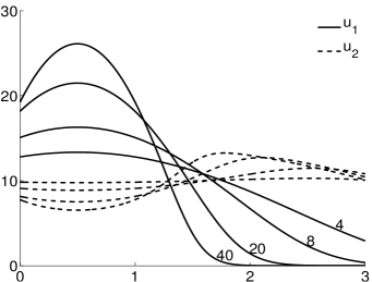
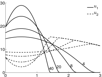
Figure 1: Experiment 1. Numerical results for several values of $b_{1}$ using Shigesada et al. model (left panel) and the model studied in this article (right panel).

Experiment 1. We compare graphically the phenomenon of segregation of populations arising from the Shigesada et al. model (2), and from the model studied in this article (9)-(11). To do this we use Example (c) of [21] in which an implicit finite differences method was used to compute the approximated solution, see also [4, 25] for the same experiment reproduced with alternative methods. The parameters are fixed as follows: $\Omega=(0,3)$, $a_{ij}=1$, $c_{i}=1$, $i,j=1,2$, $b_{2}=1$ and $b_{1}=4,~{}8,~{}20,~{}40$. The initial data is constant, $u_{i0}=10$, for $i=1,2$, and the environmental field is given by $q(x)=-3(x-0.5)$. For the Shigesada et al. model we take $M=301$ and $\tau=10^{-3}$, as in [21]. However, the convergence properties of problem (9)-(11) lead us to choose values of $M$ and $\tau$ in the range $301-1001$ and $10^{-5}-10^{-3}$, respectively, depending on the $b_{1}$ values. For both models we take tolerances $\text{tol}\sim 10^{-7}$ and $\text{tol}_{S}\leq 5\times 10^{-8}$.

In Fig. 1 we plot the approximate steady state solution for both models. Labels on curves give the corresponding $b_{1}$ value. We observe a stronger segregation effect in the model studied in this article compared to the model of Shigesada et al., although they behave similarly from a qualitative point of view. The loss of regularity of solutions when one of them vanishes is also observed. To check this fact more clearly, we run an experiment for the same data as above but: $a_{11}=4,~{}a_{12}=0,~{}a_{21}=3.9,~{}a_{22}=1$, $b_{i}=d_{i}=0$, for $i=1,2$. Observe that matrix $(a_{ij})$ satisfies the positiveness condition (14). A transient state of the solution is shown in the right panel of Fig. 6.

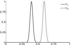
(a) $t=0$

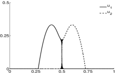
(b) $t=0.05$

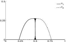
(c) $t=0.17$

Figure 2: Experiment 2. The case of semi-definite positive matrix $(a_{ij})$

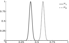
(a) $t=0$

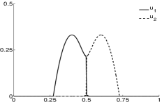
(b) $t=0.05$

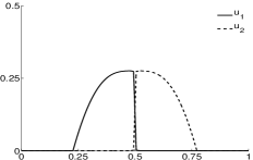
(c) $t=0.17$

Figure 3: Experiment 2. Regularizing parameter $\delta=0.001$.

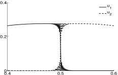
(a) $\delta=0$

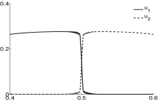
(b) $\delta=0.001$

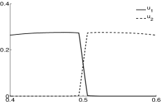
(c) $\delta=0.01$

Figure 4: Experiment 2. Zoom into the supports intersection region.

From the mathematical and numerical point of view, the most interesting situation of problem (9)-(11) is that of the degenerate case covered by assumptions (H’), i.e. when $a_{ij}=a>0$ and, therefore, matrix $(a_{ij})$ is only semi-definite positive. In this particular case, the following property holds. Let $(u_{1}^{(\delta)},u_{2}^{(\delta)})$ be a solution of problem (9)-(11) with $J_{i}$ replaced by $J_{i}^{BT,\delta}$, see (21), to which we refer to as Problem (P)_δ, and assume (H’). Then $u=u_{1}^{(\delta)}+u_{2}^{(\delta)}$ solves

$${\partial_{t}}u-\operatorname{div}J^{(\delta)}(u)=f(u) \quad\text{in }Q_{T}=\Omega\times(0,T),$$ (24)

$$J^{(\delta)}(u)\cdot n=0 \quad\text{on }\Gamma_{T}=\partial\Omega\times(0,T),$$ (25)

$$u(\cdot,0)=u_{10}+u_{20} \quad\text{in }\Omega,$$ (26)

for $J^{(\delta)}(u)=(a+\delta)u\nabla u+bqu+c\nabla u$ and $f(u)=u(\alpha-\beta u)$, which is a uniformly parabolic problem in view of (H’).

In the following experiments we take, unless otherwise stated, $\Omega=(0,1)$, $b_{i}=c_{i}=0$, and $u_{i0}=\exp((x-x_{i})^{2}/0.001)$, $f_{i}=0$ for $i=1,2$, with $x_{1}=0.4$ and $x_{2}=0.6$. We chose a larger tolerance parameter for the fixed point algorithm than in the previous experiment, $\text{tol}=10^{-4}$, in view of the slow convergence observed for the discretization parameters $M=1001$ and $\tau=10^{-5}$. Although the initial data do not satisfy condition (H’)₄, this does not seem to affect the convergence or stability of the algorithm for the different cases under study.

Experiment 2. We run experiments for solving problem (9)-(11) with coefficients $a_{ij}=1$, for $i,j=1,2$, and the corresponding regularized version given by Problem (P)_δ. We set the final time to $0.17$ and investigate the behavior of solutions during the transient state.

Due to diffusion, after a while the supports of $u_{i}$ intersect with each other at one point. In this moment, an important qualitative difference arises between the solutions of the degenerate and the regularized problems. For $\varepsilon=0$, no mixture of populations is observed at subsequent times, and a steep gradient or discontinuity is formed at the so-called contact inhibition point. Numerical instabilities are clearly seen around this point, see Fig. 2. However, since $u_{1}+u_{2}$ is a solution of problem (24)-(26) and therefore smooth and non-negative (Barenblatt type, see Theorem 2) these instabilities must remain bounded.

In Fig. 3 we plot the solution of problem (P)_δ, for $\delta=0.001$, approximating the solution of the degenerate problem shown in Figure 2. As it can be seen, instabilities do not arise (at the scale of the plot) for this regularized problem. We also observe that the components of the solution mixes in an interval of $\delta-$dependent length.

Finally, in Fig. 4 we show a zoom of the solutions of problem (9)-(11) and problems (P)_δ, for several choices of $\delta$, around the intersection point $x=0.5$. As suggested by estimate (51) (with $c=0$), the square of the $L^{2}$ norm of the gradient of the solutions seems to be proportional to, and not just bounded by, $1/\delta$.

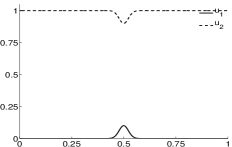
(a) $t=0$

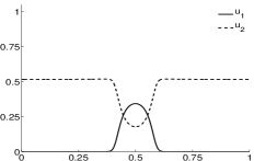
(b) $t=5$

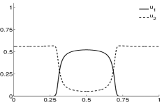
(c) $t=7$

Figure 5: Experiment 3. Evolution of the invasion.

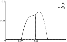
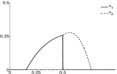
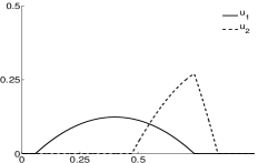
Figure 6: Experiments 4-6. Transient state profiles of solutions corresponding to: left: $d_{1}=1,~{}d_{2}=10$, center: $a_{11}=a_{12}=3$, $a_{21}=a_{22}=1$, right: $a_{11}=4,~{}a_{12}=0,~{}a_{21}=3.9,~{}a_{22}=1$.

Experiment 3. In this experiment, we look at the question (Q2) stated in [8], in which the invasion of one population (mutated abnormal cells) over an initially dominant population (normal cell) is produced. The initial data is taken as $u_{10}(x)=0.1\exp((x-x_{i})^{2}/0.001)$ and $u_{20}=1-u_{10}$. The Lotka-Volterra competitive term is taken of the usual form (13), with $\alpha_{1}=\alpha_{2}=1$, $\beta_{11}=\beta_{12}=1$ and $\beta_{21}=\beta_{22}=2$. In Fig. 6 we show the initial distributions and two instants of the transient state, in which the pressure exerted by the mutant population drives the system to a change of equilibrium. The steady state, not shown in the figure, is of extinction of the normal cells.

Experiment 4. In the following simulations we investigate other parameter ranges out of those stated in (H’). We take the same parameters than in Experiment 2 but

1. Changing matrix $(a_{ij})$ to $a_{11}=a_{12}=3$, $a_{21}=a_{22}=1$, so still positive semi-definite. We may see a transient state of the solution in the left panel of Fig. 6.

2. Changing the transport coefficients to $d_{1}=1$ and $d_{2}=10$, and setting $q(x)=-3(x-0.5)$. A transient state is plotted in the center panel of Fig. 6.

As we see, both set of parameters produce continuous solutions with discontinuous gradients at the contact inhibition point. This, again, suggests that our conditions (H’) are not optimal. In particular, a solution to the case 1. may be constructed by using Lagrangian coordinates, see [7].

5 Proofs of the theorems

5.1 Proof of Theorem 1

To make the entropy inequality (18) rigorous one has to go through a regularization procedure. We use the approach introduced by Barrett and Blowey [4], even though alternative approaches are also possible, see Chen and Jüngel [13]. Although the results in [13, 4] can not be directly applied to prove Theorem 1, we use similar techniques in its proof. For the sake of completeness, we replicate some of the arguments used in [4], showing how they adapt to problem (9)-(11) under assumptions (H).

Let $\varepsilon\in(0,1)$ and consider $F_{\varepsilon}:\mathbb{R}\to[0,\infty)$ given by

$$F_{\varepsilon}(s):=\begin{cases}\frac{s^{2}-\varepsilon^{2}}{2\varepsilon}+s(\ln\varepsilon-1)+1&\quad\text{if }s\leq\varepsilon,\\[4.30554pt] s(\ln s-1)+1&\quad\text{if }\varepsilon\leq s\leq\varepsilon^{-1},\\[4.30554pt] \frac{\varepsilon(s^{2}-\varepsilon^{-2})}{2}+s(\ln\varepsilon^{-1}-1)+1&\quad\text{if }\varepsilon^{-1}\leq s.\end{cases}$$ (27)

Notice that function $F$ given in (17) is defined in $[0,\infty)$, whereas $F_{\varepsilon}$ is defined in the whole real line, $\mathbb{R}$. Besides, $F_{\varepsilon}\in\mathcal{C}^{2,1}(\mathbb{R})$, so we may as well define the Hölder continuous function

$$\lambda_{\varepsilon}(s):=1/F^{\prime\prime}_{\varepsilon}(s).$$ (28)

The corresponding regularized version of problem (9)-(11) reads: For $i=1,2$, find $u_{\varepsilon i}:Q_{T}\to\mathbb{R}$ such that

$${\partial_{t}}u_{\varepsilon i}-\operatorname{div}J_{\varepsilon i}(u_{\varepsilon 1},u_{\varepsilon 2})=f_{\varepsilon i}(u_{\varepsilon 1},u_{\varepsilon 2}) \quad\text{in }Q_{T},$$ (29)

$$J_{\varepsilon i}(u_{\varepsilon 1},u_{\varepsilon 2})\cdot n=0 \quad\text{on }\Gamma_{T},$$ (30)

$$u_{\varepsilon i}(\cdot,0)=u_{i0} \quad\text{in }\Omega,$$ (31)

with regularized flow and competitive Lotka-Volterra functions given by

$$J_{\varepsilon i}(v_{1},v_{2})=\lambda_{\varepsilon}(v_{i})\big{(}a_{i1}\nabla v_{1}+a_{i2}\nabla v_{2}+b_{i}q)+c_{i}\nabla v_{i},$$ (32)

$$f_{\varepsilon i}(v_{1},v_{2})=\alpha_{i}v_{i}-\big{(}\beta_{i1}\lambda_{\varepsilon}(v_{1})+\beta_{i2}\lambda_{\varepsilon}(v_{2})\big{)}\lambda_{\varepsilon}(v_{i}).$$ (33)

5.1.1 Finite element approximation

We consider a fully discrete approximation using finite elements in space and backward finite differences in time. We consider a quasi-uniform family of meshes of $\Omega$ (polygonal), $\{\mathcal{T}_{h}\}_{h}$, composed by right-angled tetrahedra, with parameter $h$ representing its diameter. We introduce the finite element space of piecewise $\mathbb{P}_{1}$-elements:

$$S^{h}=\{\chi\in\mathcal{C}(\overline{\Omega});\,\chi|_{K}\in\mathbb{P}_{1}\,\text{ for all }K\in\mathcal{T}_{h}\}.$$

The Lagrange interpolation operator is denoted by $\Pi^{h}:\mathcal{C}(\overline{\Omega})\to S^{h}$. We also introduce the discrete semi-inner product on $\mathcal{C}(\overline{\Omega})$ and its induced discrete seminorm:

$$(\eta_{1},\eta_{2})^{h}=\int_{\Omega}\Pi^{h}(\eta_{1}\eta_{2}),\quad|\eta|_{h}=\sqrt{(\eta,\eta)^{h}}.$$

Finally, $Q^{h}:L^{2}(\Omega)\to S^{h}$ stands for the $L^{2}(\Omega)$-projection.

For each $\varepsilon\in(0,1)$ we consider the construction of the linear operator $\Lambda_{\varepsilon}:S^{h}\to L^{\infty}(\Omega)^{m\times m}$ given in [4, 29] which, for all $z^{h}\in S^{h}$ and a.e. in $\Omega$, has a symmetric and positive image $\Lambda_{\varepsilon}z^{h}$, and satisfies $(\Lambda_{\varepsilon}z^{h})\nabla\Pi^{h}(F_{\varepsilon}^{\prime}(z^{h}))=\nabla z^{h}$. Then, due to the right angled constraint requirement, the following bound holds

$$|\nabla\Pi^{h}\lambda_{\varepsilon}(\chi)|^{2}_{1}\leq(\nabla\chi,\nabla\Pi^{h}\lambda_{\varepsilon}(\chi))\quad\text{for all }\chi\in S^{h}.$$ (34)

For the time discretization, we take a possibly non-uniform partition of $[0,T]$ in $N$ subintervals: $0=t_{0}<t_{1}<\ldots<t_{N-1}<t_{N}=T$. We denote the time steps by $\tau_{n}=t_{n}-t_{n-1}$ ($n=1,\ldots,N$), and $\tau=\max_{n=1,\cdots,N}\tau_{n}$.

For the discrete problem we need more regularity on the coefficients than that assumed in (H). Therefore, we introduce sequences of nonnegative functions $a_{ij}^{\sigma},~{}c_{i}^{\sigma},~{}\alpha_{i}^{\sigma},~{}\beta_{ij}^{\sigma}\in\mathbb{P}_{1}([0,T];\mathcal{C}(\bar{\Omega}))$, as well as functions $b_{i}^{\sigma}\in\mathbb{P}_{1}([0,T];\mathcal{C}(\bar{\Omega}))$ and $q^{\sigma}\in(\mathbb{P}_{1}([0,T];\mathcal{C}(\bar{\Omega})))^{m}$ for $\sigma>0$, such that, as $\sigma\to 0$,

$$\begin{array}[]{l}a_{ij}^{\sigma}\to a_{ij},\quad b_{i}^{\sigma}\to b_{i},\quad c_{i}^{\sigma}\to c_{i},\quad\alpha_{i}^{\sigma}\to\alpha_{i},\quad\beta_{ij}^{\sigma}\to\beta_{ij}\quad\text{strongly in }L^{\infty}(Q_{T}),\\[1.99997pt] q^{\sigma}\to q\quad\text{strongly in }(L^{2}(Q_{T}))^{m},\end{array}$$

and satisfying (14) uniformly in $\sigma$ (i.e. with $a_{0}$ a constant independent of $\sigma$). We use the following notation for the time-space discretization of coefficients:

$$a^{\sigma n}_{ij}=\Pi^{h}(a_{ij}^{\sigma}(\cdot,t_{n})),\quad q^{\sigma n}=(\Pi^{h}(q^{\sigma}_{1}(\cdot,t_{n})),\ldots,\Pi^{h}(q^{\sigma}_{m}(\cdot,t_{n}))),\quad\text{etc.}$$

Finally, we collect here some restrictions on the discretization-regularization parameters that we shall use in this section:

$$\varepsilon\in(0,{\rm e}^{-2}),\quad h>0,\quad\sigma>0,\quad\omega\tau\leq 1-\delta<1,\quad\text{for some }\delta>0$$ (35)

with $\omega=\max_{i=1,2}\{2\|\alpha_{i}\|_{L^{\infty}(Q_{T})}+\|\beta_{i1}\|_{L^{\infty}(Q_{T})}+\|\beta_{i2}\|_{L^{\infty}(Q_{T})}\}$.

5.1.2 The discrete problem

In this subsection we prove the existence of solutions of the fully discrete problem corresponding to problem (29)-(31) and deduce uniform estimates on the solutions which will allow us to pass to the limit in the discretization-regularization problem to obtain a solution of the continuous problem. Along this subsection we omit the superindex $\sigma$ in the unknowns for clarity in the notation.

Lemma 1.

Assume (35) and let, for $n\geq 1$, $u^{n-1}_{\varepsilon i}\in S^{h}$, being $u^{0}_{\varepsilon i}:=Q^{h}u_{i0}$. Then, there exists $u^{n}_{\varepsilon i}\in S^{h}$ solution of the $n$-th step of the fully discrete problem

$$\begin{array}[]{l}\big{(}\dfrac{u^{n}_{\varepsilon i}-u^{n-1}_{\varepsilon i}}{\tau_{n}},\chi)^{h}+(\Lambda_{\varepsilon}(u^{n}_{\varepsilon i})\big{(}a_{i1}^{\sigma n}\nabla u^{n}_{\varepsilon 1}+a_{i2}^{\sigma n}\nabla u^{n}_{\varepsilon 2}+b_{i}^{\sigma n}q^{\sigma n}\big{)}+c_{i}^{\sigma n}\nabla u^{n}_{\varepsilon i},\nabla\chi)^{h}=\\[8.61108pt] \hskip 28.45274pt=(\alpha_{i}^{\sigma n}u^{n}_{\varepsilon i}-\lambda_{\varepsilon}(u^{n}_{\varepsilon i})\big{(}\beta_{i1}^{\sigma n}\lambda_{\varepsilon}(u^{n-1}_{\varepsilon 1})+\beta_{i2}^{\sigma n}\lambda_{\varepsilon}(u^{n-1}_{\varepsilon 2})\big{)},\chi)^{h},\end{array}$$ (36)

for every $\chi\in S^{h}$, and satisfying, for a constant $C$ independent of $\varepsilon$, $h$, $\tau$ and $\sigma$,

$$\begin{array}[]{l}\displaystyle\max_{n=1,\ldots,N}\Big{(}\sum_{i=1}^{2}(F_{\varepsilon}(u^{n}_{\varepsilon i}),1)^{h}+\varepsilon^{-1}|\Pi^{h}[u^{n}_{\varepsilon i}]_{-}|^{2}_{0}+|u^{n}_{\varepsilon i}|_{0,1}\Big{)}+a_{0}\sum_{n=1}^{N}\tau_{n}\sum_{i=1}^{2}||u^{n}_{\varepsilon i}||_{1}^{2}\leq C,\end{array}$$

and, for $r=2(m+1)/m$ and $p=2(m+1)/(2m+1)$,

$$\sum_{n=1}^{N}\tau_{n}\sum_{i=1}^{2}\displaystyle\Big{(}|\Lambda_{\varepsilon}(u^{n}_{\varepsilon i})|^{r}_{0,r}+|\Pi^{h}(\lambda_{\epsilon}(u^{n}_{\varepsilon i}))|^{r}_{0,r}+|u^{n}_{\varepsilon,i}|^{r}_{0,r}+|\lambda_{\varepsilon}(u^{n}_{\varepsilon i})|^{r}_{0,r}$$

$$+||\mathcal{G}(\frac{u^{n}_{\varepsilon i}-u^{n-1}_{\varepsilon i}}{\tau_{n}})||^{p}_{1,p}\displaystyle\Big{)}\leq C.$$

Proof of Lemma 1. We split the proof into three steps.

Step 1. We prove the existence of solutions of the discrete problem with a proof by contradiction. Let us define $\mathcal{A}\equiv(A_{1},A_{2}):S^{h}\times S^{h}\to S^{h}\times S^{h}$ by

$$\begin{array}[]{l}(A_{i}(v_{1},v_{2}),\chi)^{h}=(v_{i}-u^{n-1}_{\varepsilon i},\chi)^{h}+\tau_{n}\,(\Lambda_{\varepsilon}(v_{i})\big{(}a_{i1}^{\sigma n}\nabla v_{1}+a_{i2}^{\sigma n}\nabla v_{2}+b_{i}^{\sigma n}q^{\sigma n}\big{)},\nabla\chi)^{h}\\[8.61108pt] \hskip 28.45274pt+\tau_{n}(c_{i}^{\sigma n}\nabla v_{i},\nabla\chi)^{h}-\tau_{n}\,(\alpha_{i}^{\sigma n}v_{i}-\lambda_{\varepsilon}(v_{i})\big{(}\beta_{i1}^{\sigma n}\lambda_{\varepsilon}(u^{n-1}_{\varepsilon 1})+\beta_{i2}^{\sigma n}\lambda_{\varepsilon}(u^{n-1}_{\varepsilon 2})\big{)},\chi)^{h},\end{array}$$ (37)

for every $\chi\in S^{h}$. Then, the $n$-th step of the fully discrete problem, (36), consists of finding $u^{n}_{\varepsilon i}\in S^{h}$ ($i=1,2$) such that

$$\mathcal{A}(u^{n}_{\varepsilon 1},u^{n}_{\varepsilon 2})=(0,0).$$ (38)

Suppose a solution does not exist and let $R>0$ be such that

$$\sum_{i=1}^{2}|A_{i}(v_{1},v_{2})|>0\quad\text{for all }(v_{1},v_{2})\in S^{h}_{R}=\{(v_{1},v_{2})\in S^{h}\times S^{h};\,|v_{1}|_{h}^{2}+|v_{2}|_{h}^{2}\leq R^{2}\}.$$

Consider the function $B=(B_{1},B_{2}):S^{h}_{R}\to S^{h}_{R}$ given by

$$B_{i}(v_{1},v_{2}):=-R\,A_{i}(v_{1},v_{2})\big{(}\sum_{j=1}^{2}|A_{j}(v_{1},v_{2})|_{h}^{2}\big{)}^{-1/2}.$$

We have: (i) $S_{R}^{h}$ is a convex a compact subset of $S^{h}\times S^{h}$, (ii) $B$ is continuous in $S_{R}^{h}$, since $\mathcal{A}|_{S_{R}^{h}}$ is well defined and continuous, and (iii) $B(S_{R}^{h})\subset S_{R}^{h}$. Then, Brouwer’s fixed-point theorem guarantees the existence of $(w_{1},w_{2})\in S^{h}_{R}$ such that $B(w_{1},w_{2})=(w_{1},w_{2})$ which, in particular, satisfies $|w_{1}|_{h}^{2}+|w_{2}|_{h}^{2}=R^{2}$. Taking $v_{1}=w_{1}$, $v_{2}=w_{2}$ and $\chi=\Pi^{h}F_{\varepsilon}^{\prime}(w_{i})$ in (37), we obtain, using our assumption (35) on $\tau$,

$$\sum_{i=1}^{2}(A_{i}(w_{1},w_{2}),\Pi^{h}F_{\varepsilon}^{\prime}(w_{i}))^{h}\geq\frac{\varepsilon}{4}R^{2}-C,$$ (39)

with $C$ a constant independent of $\varepsilon$, $R$, $w_{1}$ and $w_{2}$. Then, for $R>0$ large enough, the following contradiction arises: On one hand, by (39) and using that $(w_{1},w_{2})$ is a fixed point of $\mathcal{B}$, we obtain

$$\sum_{i=1}^{2}(w_{i},F_{\varepsilon}^{\prime}(w_{i}))^{h}\leq-R\,\big{(}\frac{\varepsilon}{4}R^{2}-C\big{)}\big{(}\sum_{j=1}^{2}|A_{j}(w_{1},w_{2})|_{h}^{2}\big{)}^{-1/2}<0.$$

On the other hand, by standard properties of function $F_{\varepsilon}$, we deduce

$$\sum_{i=1}^{2}(w_{i},F_{\varepsilon}^{\prime}(w_{i}))^{h}\geq\sum_{i=1}^{2}\left((F_{\varepsilon}(w_{i})-F_{\varepsilon}(0),1)^{h}+\frac{\varepsilon}{2}\,|w_{i}|_{h}^{2}\right)\geq-2|\Omega|+\frac{\varepsilon}{2}\,R^{2}>0.$$

Step 2. We now pass to the proof of the first estimate of Lemma 1. Taking $\chi=\Pi^{h}F_{\varepsilon}^{\prime}(u^{n}_{\varepsilon i})$ in (36) and summing over $i=1,2$ we deduce

$$\sum_{i=1}^{2}(1-\omega\tau_{n})\,(F_{\varepsilon}(u^{n}_{\varepsilon i}),1)^{h}+\frac{a_{0}\tau_{n}}{2}\sum_{i=1}^{2}|u^{n}_{\varepsilon i}|_{1}^{2}\leq(1+\tau_{n})\,\displaystyle\sum_{i=1}^{2}(F_{\varepsilon}(u^{n-1}_{\varepsilon i}),1)^{h}+C\,\tau_{n},$$

from where we obtain

$$(1-\omega\tau_{n})\sum_{i=1}^{2}(F_{\varepsilon}(u^{n}_{\varepsilon i}),1)^{h}\leq\sum_{j=1}^{n-1}\sum_{i=1}^{2}(\tau_{j+1}+\omega\tau_{j})(F_{\varepsilon}(u^{j}_{\varepsilon i}),1)^{h}+\sum_{i=1}^{2}(F_{\varepsilon}(u^{0}_{\varepsilon i}),1)^{h}+T\,C.$$

By (35) and the discrete Gronwall’s lemma, we get

$$\max_{n=1,\ldots,N}\sum_{i=1}^{2}(F_{\varepsilon}(u^{n}_{\varepsilon i}),1)^{h}\leq\frac{1}{\delta}\,\big{(}1+T(1+\omega)\mathrm{e}^{(1+\omega)\,T}\big{)}\big{(}\sum_{i=1}^{2}(F_{\varepsilon}(u^{0}_{\varepsilon i}),1)^{h}\,(\tau+1)+T\,C\big{)}.$$ (40)

Similarly, choosing $\chi=1$ as test function in (36), leads to

$$\max_{n=1,\ldots,N}(u^{n}_{\varepsilon i},1)^{h}\leq\frac{1}{\delta}\big{(}1+\frac{\omega T}{\delta}\mathrm{e}^{\frac{\omega T}{\delta}}\big{)}\,(u^{0}_{\varepsilon i},1)^{h}.$$ (41)

Since $|u^{n}_{\varepsilon i}|_{0,1}\leq(u^{n}_{\varepsilon i},1)^{h}+2\,|\Pi^{h}[u^{n}_{\varepsilon i}]_{-}|_{0,1}$, and $|\Pi^{h}[u^{n}_{\varepsilon i}]_{-}|_{0,1}\leq C\,\varepsilon^{1/2}\,(F_{\varepsilon}(u^{n}_{\varepsilon i}),1)^{h}$, we also obtain, using (40), (41) and standard properties of function $F_{\varepsilon}$,

$$\max_{n=1,\ldots,N}|u^{n}_{\varepsilon i}|_{0,1}+\varepsilon^{-1}|\Pi^{h}[u^{n}_{\varepsilon i}]_{-}|_{0,1}^{2}\leq C.$$ (42)

Step 3. We finish the proof of the lemma proving the last estimate. Using the properties of the mapping of the reference element onto an element $K\in\mathcal{T}_{h}$ as well as Sobolev embedding theorem (for $r=2(m+1)/m$), we obtain

$$\begin{array}[]{l}|\Lambda_{\varepsilon}(u^{n}_{\varepsilon i})|_{0,r}^{r}\leq C\displaystyle\sum_{K\in\mathcal{T}_{h}}\int_{K}1\,\,|\Pi^{h}\lambda_{\varepsilon}(u^{n}_{\varepsilon i})|^{r}_{0,\infty,K}\leq C\,|\Pi^{h}\lambda_{\varepsilon}(u^{n}_{\varepsilon i})|^{r}_{0,r,\Omega}\\[4.30554pt] \hskip 85.35826pt\leq C\,|\Pi^{h}\lambda_{\varepsilon}(u^{n}_{\varepsilon i})|^{r-2}_{0,1}\,||\Pi^{h}\lambda_{\varepsilon}(u^{n}_{\varepsilon i})|^{2}_{1}.\end{array}$$

By Poincaré inequality and (34), $||\Pi^{h}\lambda_{\varepsilon}(u^{n}_{\varepsilon i})||^{2}_{1}\leq C\,(|\Pi^{h}\lambda_{\varepsilon}(u^{n}_{\varepsilon i})|^{2}_{0,1}+|u^{n}_{\varepsilon i}|^{2}_{1}).$ Besides,

$$|\Pi^{h}\lambda_{\varepsilon}(u^{n}_{\varepsilon i})|_{0,1}\leq\varepsilon\int_{\Omega}1+|u^{n}_{\varepsilon i}|_{0,1}.$$

Therefore, $|\Lambda_{\varepsilon}(u^{n}_{\varepsilon i})|_{0,r}^{r}\leq C\,(1+|u^{n}_{\varepsilon i}|^{2}_{1}).$ Moreover,

$$|\Pi^{h}\lambda_{\varepsilon}(u^{n}_{\varepsilon i})|_{0,r}^{r}+|\lambda_{\varepsilon}(u^{n}_{\varepsilon i})|_{0,r}^{r}\leq C\,(1+|u^{n}_{\varepsilon i}|^{r}_{0,r}).$$

Using $|u^{n}_{\varepsilon i}|^{r}_{0,r}\leq C\,||u^{n}_{\varepsilon i}||^{2}_{1}$, we deduce

$$|\Pi^{h}\lambda_{\varepsilon}(u^{n}_{\varepsilon i})|_{0,r}^{r}+|\lambda_{\varepsilon}(u^{n}_{\varepsilon i})|_{0,r}^{r}\leq C\,(1+||u^{n}_{\varepsilon i}||^{2}_{1}).$$

Finally, let $\mathcal{G}:(W^{1,p^{\prime}}(\Omega))^{\prime}\to W^{1,p}(\Omega)$ be given by

$$\int_{\Omega}(\nabla\mathcal{G}v\cdot\nabla w+\mathcal{G}v\,w)=\langle v,w\rangle\quad\text{for all }w\in W^{1,p^{\prime}}(\Omega),$$

being $\langle\cdot,\cdot\rangle$ the duality product ${(W^{1,p^{\prime}}(\Omega))^{\prime}\times W^{1,p^{\prime}}(\Omega)}$. From problem (36) we deduce

$$\begin{array}[]{l}\displaystyle\int_{\Omega}(\nabla\mathcal{G}\frac{u^{n}_{\varepsilon i}-u^{n-1}_{\varepsilon i}}{\tau_{n}}\cdot\nabla w+\mathcal{G}\frac{u^{n}_{\varepsilon i}-u^{n-1}_{\varepsilon i}}{\tau_{n}}\,w)=\\[6.45831pt] \hskip 28.45274pt=-(\Lambda_{\varepsilon}(u^{n}_{\varepsilon i})\big{(}a_{i1}^{\sigma n}\nabla u^{n}_{\varepsilon 1}+a_{i2}^{\sigma n}\nabla u^{n}_{\varepsilon 2}+b_{i}^{\sigma n}q^{\sigma n}\big{)}+c_{i}^{\sigma n}\nabla u^{n}_{\varepsilon i},\nabla Q^{h}w)^{h}\\[6.45831pt] \hskip 56.9055pt+(\alpha_{i}^{\sigma n}u^{n}_{\varepsilon i}-\lambda_{\varepsilon}(u^{n}_{\varepsilon i})\big{(}\beta_{i1}^{\sigma n}\lambda_{\varepsilon}(u^{n-1}_{\varepsilon 1})+\beta_{i2}^{\sigma n}\lambda_{\varepsilon}(u^{n}_{\varepsilon 2})\big{)},Q^{h}w)^{h}\end{array}$$

for $w\in W^{1,p^{\prime}}(\Omega)$. In consequence,

$$\begin{array}[]{l}\displaystyle\int_{\Omega}(\nabla\mathcal{G}\frac{u^{n}_{\varepsilon i}-u^{n-1}_{\varepsilon i}}{\tau_{n}}\cdot\nabla w+\mathcal{G}\frac{u^{n}_{\varepsilon i}-u^{n-1}_{\varepsilon i}}{\tau_{n}}\,w)\leq\\[6.45831pt] \hskip 14.22636pt\leq C\,||w||_{1,p^{\prime}}\Big{(}(1+|\Lambda_{\varepsilon}(u^{n}_{\varepsilon i})|_{0,r})\,(1+\displaystyle\sum_{j=1}^{2}|u^{n}_{\varepsilon j}|_{1})+\sum_{j=1}^{2}|\lambda_{\varepsilon}(u^{n}_{\varepsilon i})|_{0,2}\,|\lambda_{\varepsilon}(u^{n}_{\varepsilon j})|_{0,r}\Big{)}\end{array}$$

for $w\in W^{1,p^{\prime}}(\Omega)$, and therefore

$$||\mathcal{G}\frac{u^{n}_{\varepsilon i}-u^{n-1}_{\varepsilon i}}{\tau_{n}}||_{1,p}^{p}\leq C\,\Big{(}\!(1\!+\!|\Lambda_{\varepsilon}(u^{n}_{\varepsilon i})|_{0,r})\,(1\!+\!\displaystyle\sum_{j=1}^{2}|u^{n}_{\varepsilon j}|_{1})\!+\!\sum_{j=1}^{2}|\lambda_{\varepsilon}(u^{n}_{\varepsilon i})|_{0,2}|\lambda_{\varepsilon}(u^{n}_{\varepsilon j})|_{0,r}\!\Big{)}.$$

The statement follows recalling that $|\lambda_{\varepsilon}(u^{n}_{\varepsilon i})|_{0,2}\leq C\,(1+||u^{n}_{\varepsilon i}||^{2}_{1})$. $\Box$

5.1.3 Passing to the limits

In this subsection we construct the solution to the continuous problem. We make now explicit the dependence of the solution on parameter $\sigma$. For each $n=1,2,\ldots,N$, we define

$$u_{\varepsilon i}^{\sigma}(t):=\frac{t-t_{n-1}}{\tau_{n}}u_{\varepsilon i}^{\sigma n}+\frac{t_{n}-t}{\tau_{n}}u_{\varepsilon i}^{\sigma(n-1)}\quad\forall t\in[t_{n-1},t_{n}],$$ (43)

and also consider

$$(u_{\varepsilon i}^{\sigma})^{-}(t):=u_{\varepsilon i}^{\sigma(n-1)}\quad\text{and}\quad(u_{\varepsilon i}^{\sigma})^{+}(t):=u_{\varepsilon i}^{\sigma n}\quad\forall t\in(t_{n-1},t_{n}].$$ (44)

In terms of this notation, the fully discrete problem (which has a solution ensured by Lemma 1), is written as

$$\begin{array}[]{l}\displaystyle\int_{0}^{T}\Big{(}({\partial_{t}}u_{\varepsilon i}^{\sigma},\chi)^{h}+\big{(}\Lambda_{\varepsilon}((u_{\varepsilon i}^{\sigma})^{+})\big{(}a_{i1}^{\sigma}\nabla(u_{\varepsilon 1}^{\sigma})^{+}+a_{i2}^{\sigma}\nabla(u_{\varepsilon 2}^{\sigma})^{+}+b_{i}^{\sigma}q^{\sigma}\big{)}+c_{i}^{\sigma}\nabla(u_{\varepsilon i}^{\sigma})^{+},\nabla\chi\big{)}^{h}\Big{)}=\\[4.30554pt] \hskip 28.45274pt=\displaystyle\int_{0}^{T}(\alpha_{i}^{\sigma}(u_{\varepsilon i}^{\sigma})^{+}-\lambda_{\varepsilon}((u_{\varepsilon i}^{\sigma})^{+})\big{(}\beta_{i1}^{\sigma}\lambda_{\varepsilon}((u_{\varepsilon 1}^{\sigma})^{-})+\beta_{i2}^{\sigma}\lambda_{\varepsilon}((u_{\varepsilon 2}^{\sigma})^{-})\big{)},\chi)^{h}\,,\end{array}$$ (45)

$u_{\varepsilon i}\in\mathcal{C}([0,T];S^{h})$, $i=1,2$, and for every $\chi\in L^{2}((0,T);S^{h})$, and satisfying a discrete version of the initial condition:

$$u_{\varepsilon i}^{\sigma}(0)=u_{\varepsilon i}^{0}\in S^{h}.$$ (46)

Theorem 1 is a direct consequence of the uniform convergence properties of the sequence constructed through the solutions to the fully discrete problem, and stated in the following lemma. The proof of Lemma 2 mimics that of Lemma 3.1 and Theorem 3.1 of [4], and therefore we omit it.

Lemma 2.

Assume (35) and let $s\in[2,\infty]$ if $m=1$, $s\in[2,\infty)$ if $m=2$, and $s\in[2,6)$ if $m=3$. Consider regularization and discretization parameters satisfying

$$\sigma\to 0,\quad\tau\to 0,\quad\text{and}\quad\varepsilon h^{-\frac{m}{m+1}}\to 0\quad\text{as }h\to 0,$$ (47)

and the first time step satisfying $\tau_{1}\leq Ch^{2}$. Then, there exist non-negative functions $u_{i}$, $i=1,2$, with

$$u_{i}\in L^{2}((0,T);H^{1}(\Omega))\cap L^{r}(Q_{T})\cap W^{1,p}((0,T);(W^{1,p^{\prime}}(\Omega))^{\prime}),$$

such that any sequence of solutions $u_{\varepsilon i}^{\sigma}\in\mathcal{C}([0,T];S^{h})$ ($i=1,2$) of (45)-(46) has a subsequence (not relabeled) such that

$$\begin{array}[]{ll}(u_{\varepsilon i}^{\sigma})^{(\pm)}\rightharpoonup u_{i}&\quad\text{weakly in }L^{2}(0,T;H^{1}(\Omega))\cap L^{r}(Q_{T}),\\[4.30554pt] \mathcal{G}({\partial_{t}}u_{\varepsilon i}^{\sigma})\rightharpoonup\mathcal{G}({\partial_{t}}u_{i})&\quad\text{weakly in }L^{p}(0,T;W^{1,p}(\Omega)),\\[4.30554pt] (u_{\varepsilon i}^{\sigma})^{(\pm)}\to u_{i}&\quad\text{strongly in }L^{2}((0,T);L^{s}(\Omega)),\\[4.30554pt] \lambda_{\varepsilon}((u_{\varepsilon i}^{\sigma})^{\pm})\to u_{i}&\quad\text{strongly in }L^{2}((0,T);L^{r}(\Omega)),\\[4.30554pt] \Pi^{h}(\lambda_{\varepsilon}((u_{\varepsilon i}^{\sigma})^{\pm}))\to u_{i}&\quad\text{strongly in }L^{2}((0,T);L^{r}(\Omega)),\\[4.30554pt] \Lambda_{\varepsilon}((u_{\varepsilon i}^{\sigma})^{\pm})\to u_{i}\mathcal{I}&\quad\text{strongly in }L^{2}((0,T);L^{r}(\Omega)^{m\times m}).\end{array}$$

In addition, for all $\eta\in L^{p^{\prime}}((0,T);W^{1,p^{\prime}}(\Omega))$ and $i=1,2$, we have

$$\begin{array}[]{l}\displaystyle\int_{0}^{T}\Big{(}\langle{\partial_{t}}u_{i},\chi\rangle_{p^{\prime}}+\big{(}u_{i}\big{(}a_{i1}\nabla u_{1}+a_{i2}\nabla u_{2}+b_{i}q\big{)}+c_{i}\nabla u_{i},\nabla\chi\big{)}\Big{)}=\\[4.30554pt] \hskip 28.45274pt=\displaystyle\int_{0}^{T}\Big{(}(\alpha_{i}u_{i}-u_{i}\big{(}\beta_{i1}\,u_{1}+\beta_{i2}\,u_{2}\big{)},\chi)\Big{)}.\end{array}$$

5.2 Proof of Theorem 2

We consider the perturbation $J_{i}^{BT,\delta}$ introduced in (21), and recall that the following result is a consequence of Theorem 1 of [13].

Lemma 3.

Assume (H’). Then there exists a weak solution $(u_{1}^{(\delta)},u_{2}^{(\delta)})$ of problem (P)_δ in the following sense (for $i=1,2$):

• $u_{i}^{(\delta)}\geq 0$ satisfy the regularity properties

  $$\begin{array}[]{l}u_{i}^{(\delta)}\in L^{\infty}(Q_{T})\cap L^{2}(0,T;H^{1}(\Omega))\cap H^{1}(0,T;(H^{1}(\Omega))^{{}^{\prime}}).\end{array}$$

• For all $\varphi\in L^{2}(0,T;H^{1}(\Omega))$ we have

  $$\int_{0}^{T}\langle{\partial_{t}}u_{i}^{(\delta)},\varphi\rangle+\int_{Q_{T}}J_{i}^{(\delta)}(u_{1}^{(\delta)},u_{2}^{(\delta)})\cdot\nabla\varphi=\int_{Q_{T}}f_{i}(u_{1}^{(\delta)},u_{2}^{(\delta)})~{}\varphi,$$ (48)

  where $\langle\cdot,\cdot\rangle$ denotes the duality product of $(H^{1}(\Omega))^{{}^{\prime}}\times H^{1}(\Omega).$

• The initial conditions (11) are satisfied in the sense

  $$\begin{array}[]{l}\lim\|u_{i}^{(\delta)}(\cdot,t)-u_{i0}\|_{(H^{1}(\Omega))^{{}^{\prime}}}=0\end{array}\quad\text{as}\quad t\rightarrow 0.$$

In addition,

$$\|u_{1}^{(\delta)}\|_{L^{\infty}(Q_{T})}+\|u_{2}^{(\delta)}\|_{L^{\infty}(Q_{T})}+\|u_{1}^{(\delta)}+u_{2}^{(\delta)}\|_{L^{2}(0,T;H^{2}(\Omega))}\leq C,$$ (49)

with $C$ independent of $\delta$.

Proof. The proof is given in two steps. Step one consists on showing the existence of solutions of problem (P)_δ using the ideas of the problem solved by Chen and Jüngel [13], which strongly resembles ours. The only difference between both problems is in the definition of the diffusion matrices which, for the problem treated in [13] is of the form

$$A_{1}=\left(\begin{array}[]{cc}c_{1}+2a_{11}u_{1}+a_{12}u_{2}&a_{12}u_{1}\\ a_{21}u_{2}&c_{2}+2a_{22}u_{2}+a_{21}u_{1}\end{array}\right),$$

whereas for problem (P)_δ is given by

$$A_{2}=\left(\begin{array}[]{cc}c+(a+\delta)u_{1}+\frac{\delta}{2}u_{2}&(a+\frac{\delta}{2})u_{1}\\ (a+\frac{\delta}{2})u_{2}&c+(a+\delta)u_{2}+\frac{\delta}{2}u_{1}\end{array}\right),$$ (50)

which can not be recast in the form of $A_{1}$. However, as may be easily seen in [13], this difference does not affect the proof as long as the matrix resulting from the change of unknowns $u_{i}=\exp(w_{i})$ is symmetric and positive definite. And this is certainly the case since, rewriting the diffusion matrix obtained after this change of unknowns we get

$$\tilde{A}_{2}=\left(\begin{array}[]{cc}c\mathrm{e}^{w_{1}}+(a+\delta)\mathrm{e}^{2w_{1}}+\frac{\delta}{2}\mathrm{e}^{w_{1}+w_{2}}&(a+\frac{\delta}{2})\mathrm{e}^{w_{1}+w_{2}}\\ (a+\frac{\delta}{2})\mathrm{e}^{w_{1}+w_{2}}&c\mathrm{e}^{w_{2}}+(a+\delta)\mathrm{e}^{2w_{2}}+\frac{\delta}{2}\mathrm{e}^{w_{1}+w_{2}}\end{array}\right)$$

which is positive definite for all $\delta>0$. We may therefore adapt the results in [13] to obtain the existence of a solution of problem (P)_δ, but in a weaker sense than the notion of solution stated in Lemma 3.

The second step of the proof is intended to justify this point, and to this end we use that $u^{(\delta)}=u_{1}^{(\delta)}+u_{2}^{(\delta)}$ satisfies, in a weak sense, problem (24)-(26). Being this the case and recalling that assumptions (H’) imply the uniform parabolicity of problem (24)-(26), we may apply Theorem 3.1, Chapter V of [35] to deduce uniform bounds for $\|u^{(\delta)}\|_{L^{\infty}(Q_{T})}$ and $\|u^{(\delta)}\|_{L^{2}(0,T;H^{2}(\Omega))}$. In particular, the $L^{\infty}(Q_{T})$ bound on $u^{(\delta)}$ together with the non-negativity of $u_{i}^{(\delta)}$ obtained in [13] imply the uniform $L^{\infty}(Q_{T})$ bounds on $u_{i}^{(\delta)}$. In consequence, all the terms in the weak formulation (48) make sense for test functions in $L^{2}(0,T;H^{1}(\Omega))$. $\Box$

The proof of Theorem 2 is completed by passing to the limit $\delta\to 0$. Let $(u_{1}^{(\delta)},u_{2}^{(\delta)})$ be the solution of problem (P)_δ found in Lemma 3. As shown in [13], an entropy type inequality implies

$$\sum_{i=1}^{2}\int_{Q_{T}}\big{(}2c|\nabla\sqrt{u_{i}^{(\delta)}}|^{2}+\delta|\nabla u_{i}^{(\delta)}|^{2}\big{)}\leq C,$$ (51)

with $C$ independent of $\delta$. In particular, the $L^{\infty}(Q_{T})$ bound for $u_{i}^{(\delta)}$ found in Lemma 3 implies

$$\int_{Q_{T}}|\nabla u_{i}^{(\delta)}|^{2}\leq 4\|u_{i}^{(\delta)}\|_{L^{\infty}(Q_{T})}\int_{Q_{T}}|\nabla\sqrt{u_{i}^{(\delta)}}|^{2}\leq C,$$ (52)

where $C$ capture several constants independent of $\delta$. However, observe that we only assume $c\geq 0$, so bound (52) is irrelevant for the most interesting case of $c=0$. From (48) we deduce the following estimate for all $\varphi\in L^{2}(0,T;H^{1}(\Omega))$:

$$\int_{0}^{T}\langle{\partial_{t}}u_{i}^{(\delta)},\varphi\rangle\leq\|J_{i}^{(\delta)}(u_{1}^{(\delta)},u_{2}^{(\delta)})\|_{L^{2}(Q_{T})}\|\nabla\varphi\|_{L^{2}(Q_{T})}$$

$$\hskip 85.35826pt+\|f_{i}(u_{1}^{(\delta)},u_{2}^{(\delta)})\|_{L^{2}(Q_{T})}\|\varphi\|_{L^{2}(Q_{T})}.$$

We have

$$\|J_{i}^{(\delta)}(u_{1}^{(\delta)},u_{2}^{(\delta)})\|_{L^{2}(Q_{T})}\leq a\|u_{i}^{(\delta)}\|_{L^{\infty}(Q_{T})}\|\nabla(u_{1}^{(\delta)}+u_{2}^{(\delta)})\|_{L^{2}(Q_{T})}$$

$$+|b|\|u_{i}^{(\delta)}\|_{L^{\infty}(Q_{T})}\|q\|_{L^{2}(Q_{T})}+c\|\nabla u_{i}^{(\delta)}\|_{L^{2}(Q_{T})}+\delta\|u_{i}^{(\delta)}\|_{L^{\infty}(Q_{T})}\|\nabla u_{i}^{(\delta)}\|_{L^{2}(Q_{T})}$$

$$+\frac{\delta}{2}\Big{(}\|u_{1}^{(\delta)}\|_{L^{\infty}(Q_{T})}\|\nabla u_{2}^{(\delta)}\|_{L^{2}(Q_{T})}+\|u_{2}^{(\delta)}\|_{L^{\infty}(Q_{T})}\|\nabla u_{1}^{(\delta)}\|_{L^{2}(Q_{T})}\Big{)}.$$

Using the $L^{\infty}(Q_{T})$ uniform estimates in (49), bound (52) and assumptions (H’) we get

$$\int_{0}^{T}\langle{\partial_{t}}u_{i}^{(\delta)},\varphi\rangle\leq C_{1}\Big{(}1+\|\nabla(u_{1}^{(\delta)}+u_{2}^{(\delta)})\|_{L^{2}(Q_{T})}\Big{)}\|\nabla\varphi\|_{L^{2}(Q_{T})}+C_{2}\|\varphi\|_{L^{2}(Q_{T})}$$

$$+\delta C_{3}\big{(}\|\nabla u_{1}^{(\delta)}\|_{L^{2}(Q_{T})}+\|\nabla u_{2}^{(\delta)}\|_{L^{2}(Q_{T})}\big{)}\|\nabla\varphi\|_{L^{2}(Q_{T})},$$

and from the $L^{2}(Q_{T})$ uniform estimates for $\nabla(u_{1}^{(\delta)}+u_{2}^{(\delta)})$ in (49) and estimate (51) we deduce

$$\|{\partial_{t}}u_{i}^{(\delta)}\|_{L^{2}(0,T;(H^{1}(\Omega))^{\prime}}\leq C(1+\sqrt{\delta}).$$ (53)

Thus, using (49), (51) and (53), we deduce the existence of subsequences (not relabeled) and functions $u_{i}\in H^{1}(0,T;L^{2}(\Omega))\cap L^{\infty}(Q_{T})$ and $u\in H^{1}(0,T;L^{2}(\Omega))\cap L^{2}(0,T;H^{2}(\Omega))\cap L^{\infty}(Q_{T})$ such that (see [46])

$${\partial_{t}}u_{i}^{(\delta)}\rightharpoonup{\partial_{t}}u_{i}\quad\text{weakly in }L^{2}(0,T;(H^{1}(\Omega))^{\prime}),$$

$$u_{i}^{(\delta)}\overset{*}{\rightharpoonup}u_{i}\quad\text{weakly * in }L^{\infty}(Q_{T}),$$ (54)

$$\nabla(u_{1}^{(\delta)}+u_{2}^{(\delta)})\to\nabla u\quad\text{strongly in }L^{2}(Q_{T}),$$ (55)

$$u_{1}^{(\delta)}+u_{2}^{(\delta)}\to u\quad\text{strongly in }L^{2}(Q_{T}).$$ (56)

As a first observation, we may identify $u$ as $u_{1}+u_{2}$ due to (54) and (56). Using estimate (51) and the uniform $L^{\infty}(Q_{T})$ estimate of $u_{i}^{(\delta)}$ in (49) we also deduce, for $i,j=1,2$ ,

$$\delta\int_{Q_{T}}u_{i}^{(\delta)}\nabla u_{j}^{(\delta)}\cdot\nabla\varphi\leq\delta\|u_{i}^{(\delta)}\|_{L^{\infty}(Q_{T}))}\|\nabla u_{j}^{(\delta)}\|_{L^{2}(Q_{T}))}\|\nabla\varphi\|_{L^{2}(Q_{T}))}\leq C\sqrt{\delta}.$$

Finally, in the passing to the limit $\delta\to 0$ in (48) there are only two non-standard terms,

$$\int_{Q_{T}}u_{i}^{(\delta)}\nabla{(u_{1}^{(\delta)}+u_{2}^{(\delta)})}\cdot\nabla\varphi$$

and

$$\int_{Q_{T}}f_{i}(u_{1}^{(\delta)},u_{2}^{(\delta)})\varphi=\int_{Q_{T}}u_{i}^{(\delta)}(\alpha-\beta(u_{1}^{(\delta)}+u_{2}^{(\delta)})\varphi,$$

which converge to their corresponding limits in view of (54)-(56). $\Box$

6 Conclusion

We have shown that a natural election for cross-diffusion modeling, from the point of view of limit densities corresponding to systems of particles, is that introduced by Busenberg and Travis [10] from macroscopic ad-hoc considerations, in the discipline of population dynamics. Although a rigorous deduction for boundary value problems has not been accomplished yet, the results for the Cauchy problem seems to point to the model considered in this article. Mathematically, the problem of existence of solutions has two cases. The first is the case in which the system matrix $(a_{ij})$ is positive definite, for which we have given a rather general proof based on previous results for the Shigesada et al. model [45]. The second, is the case in which this matrix is only positive semi-definite. We have given a partial result of existence of solutions which generalizes previous results based on the solution construction by Lagrangian flows. In this case, the problem is specially interesting for segregated initial data, giving rise to the contact inhibition problem arising from tumor modeling. After checking the qualitative similarities, from a numerical simulation point of view, between the BT and the SKT models when the problem is parabolic (positive definite matrix), we have reviewed several situations in which the presumably non-parabolic problem (positive semi-definite matrix) gives rise to discontinuous solutions. We have also performed simulations out of the range of the assumptions for the existence proof, showing that they seem to be just technical restrictions. In future work, we shall investigate the possibilities of broadening such conditions.

References

• [1] S. Aly, M. Farkas, Competition in patchy environment with cross diffusion, Nonlinear Anal. Real World Appl. 5(4) (2004) 589–595.
• [2] M. Andreianov, B. Bendahmane, R. Ruiz-Baier, Analysis of a finite volume method for a cross-diffusion model in population dynamics, Math. Mod. Meth. Appl. Sci. 21(2) (2011) 307–344.
• [3] I. S. Aranson, L. S. Tsimring, Continuum theory of partially fluidized granular flows, Phys. Rev. E (3) 65 (2002) 061303.
• [4] J. W. Barrett, J. F. Blowey, Finite element approximation of a nonlinear cross-diffusion population model, Numer. Math. 98 (2004) 195–221.
• [5] M. Bendahmane, Weak and classical solutions to predator-prey system with cross-diffusion, Nonlinear Anal. 73 (2010) 2489–2503.
• [6] S. Berres, R. Ruiz-Baier, A fully adaptive numerical approximation for a two-dimensional epidemic model with nonlinear cross-diffusion, Nonlinear Anal. Real World Appl. 12 (2011) 2888–2903.
• [7] M. Bertsch, M. E. Gurtin, D. Hilhorst, L. A. Peletier, On interacting populations that disperse to avoid crowding: preservation of segregation, J. Math. Biol. 23 (1985) 1–13
• [8] M. Bertsch, R. Dal Passo, M. Mimura, A free boundary problem arising in a simplified tumour growth model of contact inhibition, Interface Free Bound. 12 (2010) 235–250.
• [9] M. Bertsch, D. Hilhorst, H. Izuhara, M. Mimura, A nonlinear parabolic-hyperbolic system for contact inhibition of cell-growth, Diff. Equ. Appl. 4 (2012) 137–157.
• [10] S. N. Busenberg, C. C. Travis, Epidemic models with spatial spread due to population migration, J. Math. Biol. 16 (1983) 181–198.
• [11] V. Capasso, D. Morale, Rescaling stochastic processes: asymptotics, in: V. Capasso, M. Lachowicz (Eds.), Multiscale Problems in the Life Sciences. From Microscopic to Macroscopic, in: Lecture Notes in Mathematics Springer (2008) 91–146.
• [12] M. Chaplain, L. Graziano, L. Preziosi, Mathematical modelling of the loss of tissue compression responsiveness and its role in solid tumour development, Math. Med. Biol. 23 (2006) 197–229.
• [13] L. Chen, A. Jüngel, Analysis of a multidimensional parabolic population model with strong cross-diffusion, SIAM J. Math. Anal. 36(1) (2004) 301–322.
• [14] L. Chen, A. Jüngel, Analysis of a parabolic cross-diffusion semiconductor model with electron-hole scattering, Comm. Partial Differential Equations, 32 (2007) 127–148.
• [15] R. Cherniha, L. Myroniuk, New exact solutions of a nonlinear cross-diffusion system, J. Phys. A: Math. Theor. 41(39) (2008) 395–204.
• [16] P. Degond, S. Genieys, Jüngel, A system of parabolic equations in nonequilibrium thermodynamics including thermal and electrical effects, J. Math. Pures Appl. 76(10) (1997) 991–1015.
• [17] D. del Castillo-Negrete, B. A. Carreras, V. Lynch, Front propagation and segregation in a reaction-diffusion model with cross-diffusion, Phys. D, 168-169 (2002) 45–60.
• [18] P. Deuring, An initial-boundary value problem for a certain density-dependent diffusion system, Math. Z. 194 (1987) 375-396.
• [19] A. Friedman, Stochastic differential equations and applications. Vols. I and II, Academic Press, London, 1975.
• [20] G. Galiano, On a cross-diffusion population model deduced from mutation and splitting of a single species, Comput. Math. Appl. 64(6) (2012) 1927-1936.
• [21] G. Galiano, M. L. Garzón, A. Jüngel, Analysis and numerical solution of a nonlinear cross-diffusion system arising in population dynamics, RACSAM Rev. R. Acad. Cienc. Exactas Fís. Nat. Ser. A Mat. 95(2) (2001) 281–295.
• [22] G. Galiano, M. L. Garzón, A. Jüngel, Semi-discretization in time and numerical convergence of solutions of a nonlinear cross-diffusion population model, Numer. Math. 93(4) (2003) 655–673.
• [23] G. Galiano, A. Jüngel, J. Velasco, A parabolic cross-diffusion system for granular materials, SIAM J. Math. Anal. 35(3) (2003) 561–578.
• [24] G. Galiano, J. Velasco, Competing through altering the environment: A cross–diffusion population model coupled to transport-darcy flow equations, Nonlinear Anal. Real World Appl. 12(5) (2011) 2826–2838.
• [25] G. Gambino, M.C. Lombardo and M. Sammartino, A velocity-diffusion method for a Lotka-Volterra system with nonlinear cross and self-diffusion, Appl. Numer. Math. 59 (2009) 1059–1074.
• [26] G. Gambino, M.C. Lombardo and M. Sammartino, Turing instability and traveling fronts for a nonlinear reaction–diffusion system with cross-diffusion Original, Math. Comput. Simul.82(6) (2012) 1112–1132.
• [27] G. Gambino, M.C. Lombardo and M. Sammartino, Pattern formation driven by cross–diffusion in a 2D domain, Nonlinear Anal. Real World Appl. 14(3) (2013) 1755–1779.
• [28] E. Gilad, J. von Hardenberg, A. Provenzale, M. Shachak, E. Meron. A mathematical model of plants as ecosystem engineers, J. Theoret. Biol. 244(4) (2007) 680–691.
• [29] G. Grün, M. Rumpf, Nonnegativity preserving convergent schemes for the thin film equation, Numer. Math. 87 (2000) 113–152.
• [30] M. E. Gurtin, A. C. Pipkin, On interacting populations that disperse to avoid crowding, Q. Appl. Math. 42 (1984) 87–94.
• [31] J. Jorné, The diffusive Lotka-Volterra oscillating system, J. Theor. Biol. 65 (1977) 133–139.
• [32] E. H. Kerner, Further considerations on the statistical mechanics of biological associations, Bull. Math. Biophys. 21 (1959) 217–255.
• [33] J. U. Kim, Smooth solutions to a quasi-linear system of diffusion equations for a certain population model, Nonlinear Anal. 8 (1984) 1121–1144.
• [34] M. Lachowicz, Individually-based Markov processes modeling nonlinear systems in mathematical biology, Nonlinear Anal. Real World Appl. 12 (2011) 2396–2407.
• [35] O. A. Ladyzenskaja, V. A. Solonnikov, N. N. Ural’ceva, Linear and quasilinear equations of parabolic type, AMS, Providence, 1968.
• [36] P. L. Lions, A. S. Sznitman, Stochastic differential equations with reflecting boundary conditions, Comm. Pure Appl. Math. 37(4) (1984) 511–537.
• [37] Y. Lou, W. M. Ni, Y. Wu, Diffusion, self-diffusion and cross-diffusion, J. Differ. Equations 131(1) (1996) 79–131.
• [38] Y. Lou, W. M. Ni, Y. Wu, The global existence of solutions for a cross-diffusion system, Adv. Math. Beijing 25 (1996) 283-284.
• [39] H.C. Marques, J.J. Arenzon, Y. Levin, M. Sellitto, A nonlinear diffusion model for granular segregation, Phys. A 327 (2003) 94–98.
• [40] D. Morale, V. Capasso, K. Oelschläger, An interacting particle system modeling aggregation behavior: from individuals to populations, J. Math. Biol. 50 (2005) 49–66.
• [41] K. Oelschläger, On the derivation of reaction-diffusion equations as limit dynamics of systems of moderately interacting stochastic processes, Prob. Th. Rel. Fields 82 (1989) 565–586.
• [42] A. Okubo, S. A. Levin, Diffusion and ecological problems, Second ed., Springer-Verlag, New York, 2001.
• [43] R. Ruiz-Baier, C. Tian, Mathematical analysis and numerical simulation of pattern formation under cross-diffusion, Nonlinear Anal. Real World Appl. 14(1) (2013) 601–612.
• [44] J. A. Sherratt, Wavefront propagation in a competition equation with a new motility term modelling contact inhibition between cell populations, R. Soc. Lond. Proc. Ser. A Math. Phys. Eng. Sci. 456 (2000) 2365–2386.
• [45] N. Shigesada, K. Kawasaki, E. Teramoto, Spatial segregation of interacting species, J. Theor. Biol. 79 (1979) 83–99.
• [46] J. Simon, Compact sets in the space $L^{p}(0,T;B)$, Ann. Math. Pura et Appl. 146 (1987) 65-96.
• [47] A. Singer, Z. Schuss, A. Osipov, D. Holcman, Partially reflected diffusion, SIAM J. Appl. Math. 68(3) (2008) 844–868.
• [48] L. Slomiński, On existence, uniqueness and stability of solutions of multidimensional SDE’s with reflecting boundary conditions, Ann. Inst. H. Poincaré 29(2) (1993) 163–198.
• [49] A. Stevens, The derivarion of chemotaxis equations as limit dynamics of moderately interacting stochastic many-particles systems, SIAM J. Appl. Math. 61(1) (2000) 183–212.
• [50] C. Tian, Z. Lin, M. Pedersen, Instability induced by cross-diffusion in reaction-diffusion systems, Nonlin. Anal. RWA 11 (2010) 1036–1045.
• [51] V.K. Vanag, I.R. Epstein, Cross-diffusion and pattern formation in reaction–diffusion system, Phys. Chem. Chem. Phys. 11 (2009) 897–912.
• [52] Z. Wen, S. Fu Global solutions to a class of multi-species reaction–diffusion systems with cross-diffusions arising in population dynamics, J. Comput. Appl. Math. 230(1) (2009) 34–43.
• [53] Y. Wu, X. Zhao, The existence and stability of travelling waves with transition layers for some singular cross-diffusion systems, Phys. D, 200 (2005) 325–358.
• [54] A. Yagi, Global solution to some quasilinear parabolic system in population dynamics, Nonlinear Anal. 21 (1993) 603–630.
• [55] J.F. Zhang, W.T. Li, Y.X. Wang, Turing patterns of a strongly coupled predator-prey system with diffusion effects, Nonlin. Anal. 74 (2011) 847–858.