Deterministic particle method approximation of a contact inhibition cross-diffusion problem

Abstract

We use a deterministic particle method to produce numerical approximations to the solutions of an evolution cross-diffusion problem for two populations.

According to the values of the diffusion parameters related to the intra and inter-population repulsion intensities, the system may be classified in terms of an associated matrix. When the matrix is definite positive, the problem is well posed and the Finite Element approximation produces convergent approximations to the exact solution.

A particularly important case arises when the matrix is only positive semi-definite and the initial data are segregated: the contact inhibition problem. In this case, the solutions may be discontinuous and hence the (conforming) Finite Element approximation may exhibit instabilities in the neighborhood of the discontinuity.

In this article we deduce the particle method approximation to the general cross-diffusion problem and apply it to the contact inhibition problem. We then provide some numerical experiments comparing the results produced by the Finite Element and the particle method discretizations.

• Keywords: Cross-diffusion system, contact inhibition problem, deterministic particle method, finite element method, numerical simulations.

• AMS: 35K55, 35D30, 92D25.

1 Introduction

In this article, we shall study the numerical approximation to the following problem: Given a fixed $T>0$ and a bounded set $\Omega\subset\mathbb{R}^{m}$, find $u_{i}:\Omega\times(0,T)\to\mathbb{R}$ such that, for $i=1,2$,

$${\partial_{t}}u_{i}-\operatorname{div}J_{i}(u_{1},u_{2})=f_{i}(u_{1},u_{2}) \quad\text{in }Q_{T}=\Omega\times(0,T),$$ (1)

$$J_{i}(u_{1},u_{2})\cdot n=0 \quad\text{on }\Gamma_{T}=\partial\Omega\times(0,T),$$ (2)

$$u_{i}(\cdot,0)=u_{i0} \quad\text{in }\Omega,$$ (3)

with flow and competitive Lotka-Volterra functions given by

$$J_{i}(u_{1},u_{2})=u_{i}\big{(}a_{i1}\nabla u_{1}+a_{i2}\nabla u_{2}+b_{i}q\big{)}+c_{i}\nabla u_{i},$$ (4)

$$f_{i}(u_{1},u_{2})=u_{i}\big{(}\alpha_{i}-\beta_{i1}u_{1}-\beta_{i2}u_{2}\big{)},$$ (5)

where, for $i,j=1,2$, the coefficients $a_{ij},~{}c_{i},~{}\alpha_{i},~{}\beta_{ij}$ are non-negative constants, $b_{i}$ is a real constant, $q:\Omega\times(0,T)\to\mathbb{R}^{m}$, and $u_{i0}$ are non-negative functions.

Problem (1)-(5) is a generalization of the cross-diffusion model introduced by Busenberg and Travis [9] and Gurtin and Pipkin [27] to take into account the effect of over-crowding repulsion on the population dynamics, see [20] for the modelling details.

Under the main condition

$$4a_{11}a_{22}-(a_{12}+a_{21})^{2}>a_{0}\quad\text{a.e. in }Q_{T}.$$ (6)

for some positive constant $a_{0}$, it was proven in [20] the existence of weak solutions for rather general conditions on the data problem. Notice that (6) implies the following ellipticity condition on the matrix $A=(a_{ij})_{i,j=1}^{2}$:

$$\xi^{T}A~{}\xi\geq a_{0}\|\xi\|^{2}\quad\text{for all }\xi\in\mathbb{R}^{2}.$$

This condition allows us to, through a procedure of approximation, justify the use of $\ln u_{i}$ as a test function in the weak formulation of (1)-(3). Then we get, for the entropy functional

$$E(t)=\sum_{i=1}^{2}\int_{\Omega}F(u_{i}(\cdot,t))\geq 0,\quad\text{with }F(s)=s(\ln s-1)+1,$$

the identity

$$E(t)+\int_{Q_{t}}\Big{(}\sum_{i=1}^{2}(a_{ii}|\nabla u_{i}|^{2}+2c_{i}|\nabla\sqrt{u_{i}}|^{2})+(a_{12}+a_{21})\nabla u_{1}\cdot\nabla u_{2}\Big{)}$$

$$=E(0)+\int_{Q_{t}}\sum_{i=1}^{2}\Big{(}-b_{i}\,q\cdot\nabla u_{i}+f_{i}(u_{1},u_{2})\ln u_{i}\Big{)}.$$

From (6) and other minor assumptions one then obtains the entropy inequality

$$E(t)+a_{0}\int_{Q_{t}}(|\nabla u_{1}|^{2}+|\nabla u_{2}|^{2})\leq(E(0)+C_{1})\,\mathrm{e}^{C_{2}t},$$

providing the key $L^{2}(0,T;H^{1}(\Omega­))$ estimate of $u_{1}$ and $u_{2}$ which allows to prove the existence of weak solutions.

However, it was also proven in [20] that condition (6) is just a sufficient condition, and that solutions may exist for the case of semi-definite positive matrix $A$.

A particular important case captured by problem (1)-(5) is the contact inhibition problem, arising in tumor modeling, see for instance Chaplain et al. [10]. In this case, matrix $A$ is semi-definite positive, and the initial data, describing the spatial distribution of normal and tumor tissue, satisfy $\{u_{10}>0\}\cap\{u_{20}>0\}=\emptyset$.

This free boundary problem was mathematically analyzed by Bertsch et al. for one [7] and several spatial dimensions [8] by using regular Lagrangian flow techniques. In [20], a different approach based on viscosity perturbations was used to prove the existence of solutions. In [21], the Lagrangian techniques of [8] were generalized showing, in particular, the non-uniqueness in the construction of solutions by this method.

In [20], a conforming Finite Element Method was used both for proving the existence of solutions of the viscosity approximations (or for the case of $A$ satisfying (6)), and for the numerical simulation of solutions. Since in the case of positive semi-definite matrix $A$ solutions may develope discontinuities in finite time, the FEM approximations exhibit instabilities in the neighborhood of these points. In this article we use a deterministic particle method to give an alternative for the numerical simulation of solutions.

In our context, deterministic particle methods were introduced, for the scalar linear diffusion equation, by Degond and Mustieles in [13, 14]. Lions and Mas-Gallic, in [29], gave a rigorous justification of the method with a generalization to nonlinear diffusion. Gambino et al. [23] studied a particle approximation to a cross-diffusion problem closely related to ours.

Let us finally remark that cross-diffusion parabolic systems have been used to model a variety of phenomena since the seminal work of Shigesada, Kawaski and Teramoto [34]. These models ranges from ecology [26, 35, 22, 16, 33], to semiconductor theory [12] or granular materials [2, 19], among others. Global existence and regularity results for the evolution problem [28, 15, 36, 17, 18, 11, 5, 16], and for the steady state [30, 31] have been provided. Other interesting properties, such as pattern formation, has been studied in [24, 32, 25]. Finally, the numerical discretization has received much attention, and several schemes have been proposed [17, 18, 4, 23, 1, 6].

2 The particle method

Consider a system of $2N$ particles described by ther masses, $w_{k}^{i}>0$, and their trajectories, $x_{k}^{i}:[0,T]\to\Omega\subset\mathbb{R}^{m}$, for $k=1,\ldots,N$ (particle labels) and $i=1,2$ (populations). On one hand, the individual particles state may be modeled by Dirac delta measures

$$\epsilon_{x^{i}_{j}(t)}(B)=\left\{\begin{array}[]{ll}1&\text{if }x^{i}_{k}(t)\in B\\ 0&\text{if }x^{i}_{k}(t)\notin B\end{array}\right.\quad\text{for all }B\in{\mathcal{B}}(\mathbb{R}^{m}),$$

where ${\mathcal{B}}(\mathbb{R}^{m})$ denotes the Borel $\sigma-$algebra generated by open sets in $\mathbb{R}^{m}$. On the other hand, the collective behavior of the discrete system may be given in terms of the spatial distribution of particles at time $t$, expressed through the empirical measures

$$u^{N}_{i}(t)=\sum_{j=1}^{N}w_{k}^{i}\epsilon_{x^{i}_{k}(t)},$$

which give the spatial relative frequency of particles of the $i$-th population, at time $t$.

Using the weak formulation of (1)-(3) and assuming, for the moment, $f_{i}=0$, we find that $x_{k}^{i}$ satisfy, formally

$$\frac{d}{dt}x_{k}^{i}(t)=\frac{1}{u_{i}^{N}(x_{k}^{i}(t))}J_{i}(u_{1}^{N}(x_{k}^{i}(t)),u_{2}^{N}(x_{k}^{i}(t))).$$ (7)

We may then initialize this system of ODE’s with a suitable particle approximation of the initial data $u_{i0}$ to find an approximation to the solution of problem (1)-(3).

Since the Dirac delta measure is difficult to handle, one usually introduces a regularizing non-negative symmetric kernel $\xi_{\varepsilon}$ such that $\xi_{\varepsilon}(x)=\varepsilon^{-m}\xi(x/\varepsilon)$, with $\int_{\mathbb{R}^{m}}\xi=1$ and $\xi_{\varepsilon}\to\delta$ as $\varepsilon\to 0$, where $\delta$ denotes the Dirac delta distribution. The Gaussian kernel is a common choice.

Then, we look for functions

$$u_{i}^{N,\varepsilon}(x,t)=\sum_{k=1}^{N}w_{k}^{i}\xi_{\varepsilon}(x-x^{i}_{k}(t))$$ (8)

such that (7) is satisfied with $u_{i}^{N}$ replaced by $u_{i}^{N,\varepsilon}$, i.e.

$$\left\{\begin{array}[]{ll}\dfrac{d}{dt}x_{k}^{i}(t)=-\Big{(}a_{i1}\nabla u_{1}^{N,\varepsilon}(x_{k}^{i}(t))+a_{i2}\nabla u_{2}^{N,\varepsilon}(x_{k}^{i}(t))+c_{i}\dfrac{\nabla u_{i}^{N,\varepsilon}(x_{k}^{i}(t))}{u_{i}^{N,\varepsilon}(x_{k}^{i}(t))}+b_{i}q\Big{)},\\ x_{k}^{i}(0)=x_{0k}^{i},\end{array}\right.$$ (9)

for $i=1,2$, and with $x_{0k}^{i}$ such that $u_{i}^{N,\varepsilon}(x,0)$ is a suitable approximation to the initial data $u_{i0}(x)$ . In the formula above, the gradients are computed as

$$\nabla u_{i}^{N,\varepsilon}(x,t)=\sum_{k=1}^{N}w_{k}^{i}\nabla\xi_{\varepsilon}(x-x^{i}_{k}(t)).$$

Observe that he existence and uniqueness of solution to problem (9) is guaranteed by the Lipschitz continuity of the right hand side term.

2.1 Implementation

For the implementation details, we consider the one-dimensional spatial case, i.e. $m=1$. Let us introduce some notation.

Let $\Omega=(a,b)$. Problem (9) may be rewritten as: For $i=1,2$, find $\mathbf{x}^{i}(t):=(x^{i}_{k}(t))_{k=1}^{N}:[0,T]\to\Omega^{N}$ and $\mathbf{w}^{i}:=(w^{i}_{k})_{k=1}^{N}$ with $w^{i}_{k}>0$, satisfying

$$\left\{\begin{array}[]{l}\dfrac{d\,}{dt}\mathbf{x}^{i}(t)=\mathbf{g}^{i}(t,\mathbf{x}^{1}(t),\mathbf{w}^{1},\mathbf{x}^{2}(t),\mathbf{w}^{2})\quad\text{for }t\in(0,T)\,,\\[4.30554pt] \mathbf{x}^{i}(0)=\mathbf{x}^{i}_{0},\end{array}\right.$$ (10)

where

$$\begin{array}[]{ll}g^{i}_{k}(s,\mathbf{y}^{1},\mathbf{v}^{1},\mathbf{y}^{2},\mathbf{v}^{2}):=&-\Big{(}a_{i1}\nabla u^{N,\varepsilon}(y_{k}^{i};\mathbf{y}^{1},\mathbf{v}^{1})+a_{i2}\nabla u^{N,\varepsilon}(y_{k}^{i};\mathbf{y}^{2},\mathbf{v}^{2})\Big{.}\\ &\qquad\Big{.}+c_{i}\frac{\nabla u^{N,\varepsilon}(y_{k}^{i};\mathbf{y}^{i},\mathbf{v}^{i})}{u^{N,\varepsilon}(y_{k}^{i};\mathbf{y}^{i},\mathbf{v}^{i})}+b_{i}q(y^{i}_{k},s)\Big{)},\end{array}$$

for any $\mathbf{y}^{1},\mathbf{v}^{1},\mathbf{y}^{2},\mathbf{v}^{2}\in\mathbb{R}^{N}$ and $s\in(0,T)$, and we introduced the following generalized counterpart of (8):

$$u^{N,\varepsilon}(x;\mathbf{y},\mathbf{v})=\sum_{k=1}^{N}v_{k}\,\xi_{\varepsilon}(x-y_{k})\quad\forall\mathbf{y},\mathbf{v}\in\mathbb{R}^{N},\,x\in\mathbb{R}\,.$$

Notice that, so defined, function $\mathbf{g}^{i}$ may lead to numerical instabilities when $u^{N,\varepsilon}(y_{k}^{i};\mathbf{y}^{i},\mathbf{v}^{i})$ cancels; thus, to avoid divisions by zero, we introduce a parameter $\tilde{\varepsilon}>0$ small enough and approximate $g^{i}_{k}(s,\mathbf{y}^{1},\mathbf{v}^{1},\mathbf{y}^{2},\mathbf{v}^{2})$ by

$$\begin{array}[]{ll}\tilde{g}^{i}_{k}(s,\mathbf{y}^{1},\mathbf{v}^{1},\mathbf{y}^{2},\mathbf{v}^{2}):=&-\Big{(}a_{i1}\nabla u^{N,\varepsilon}(y_{k}^{i};\mathbf{y}^{1},\mathbf{v}^{1})+a_{i2}\nabla u^{N,\varepsilon}(y_{k}^{i};\mathbf{y}^{2},\mathbf{v}^{2})\Big{.}\\ &\qquad\Big{.}+c_{i}\frac{u^{N,\varepsilon}(y_{k}^{i};\mathbf{y}^{i},\mathbf{v}^{i})\,\nabla u^{N,\varepsilon}(y_{k}^{i};\mathbf{y}^{i},\mathbf{v}^{i})}{(u^{N,\varepsilon}(y_{k}^{i};\mathbf{y}^{i},\mathbf{v}^{i}))^{2}+\tilde{\varepsilon}^{2}}+b_{i}q(y^{i}_{k},s)\Big{)}.\end{array}$$

In order to approximate system (10), we apply a time discretization based on an implicit midpoint formula. More precisely, we fix a constant time step $\Delta t=T/M$ ($M\in\mathbb{N}$) and, given ${u}^{i,n}\approx{u}^{i}(t_{n})$ a particle approximation with the associated positions $\mathbf{x}^{i,n}\approx\mathbf{x}^{i}(t_{n})$ ($i=1,2$) and weights $\mathbf{w}^{i}$, we approximate $u^{i,n+1}\approx u^{i}(t_{n+1})$ as follows:

1. Approximate the position of the associated particles at time $t_{n+1/2}$, $\mathbf{x}^{i,n+1/2}\approx\mathbf{x}^{i}(t_{n+1/2})$, using an implicit Euler rule:

   $$\mathbf{x}^{i,n+1/2}=\mathbf{x}^{i,n}+\frac{\Delta t}{2}\,\tilde{\mathbf{g}}^{i}(t_{n+1/2},\mathbf{x}^{1,n+1/2},\mathbf{w}^{1},\mathbf{x}^{2,n+1/2},\mathbf{w}^{2})\,.$$ (11)

2. Approximate the position of the associated particles at time $t_{n+1}$, $\mathbf{x}^{i,n+1}\approx\mathbf{x}^{i}(t_{n+1})$, using an explicit Euler rule:

   $$\mathbf{x}^{i,n+1}=\mathbf{x}^{i,n+1/2}+\frac{\Delta t}{2}\,\tilde{\mathbf{g}}^{i}(t_{n+1/2},\mathbf{x}^{1,n+1/2},\mathbf{w}^{1},\mathbf{x}^{2,n+1/2},\mathbf{w}^{2})\,.$$

3. Approximate $u^{i,n+1}\approx u^{i}(t_{n+1})$ taking advantage of the approximate position of the associated particles $\mathbf{x}^{i,n+1}$:

   $$u^{i,n+1}:=u^{N,\varepsilon}(\cdot;\mathbf{x}^{i,n+1},\mathbf{w}^{i})\,.$$

Notice that the first step above requires the determination of the solution of the nonlinear algebraic equation (11). We compute an approximation to such solution by applying a fixed point algorithm. It consists of the following steps:

1. Initialize $\mathbf{x}^{i,n+1/2,1}:=\mathbf{x}^{i,n}$.

2. For $j=1,2,\ldots$, given $\mathbf{x}^{i,n+1/2,j}$,

   $$\mathbf{x}^{i,n+1/2,j+1}=\mathbf{x}^{i,n}+\frac{\Delta t}{2}\,\tilde{\mathbf{g}}^{i}(t_{n+1/2},\mathbf{x}^{1,n+1/2,j},\mathbf{w}^{1},\mathbf{x}^{2,n+1/2,j},\mathbf{w}^{2})\quad(i=1,2)\,.$$

3. Check the stopping criteria,

   $$\max_{i=1,2}\max_{x\in C_{N}}|u_{i}^{N,\varepsilon}(x;\mathbf{x}^{i,n+1/2,j+1},\mathbf{w}^{i})-u_{i}^{N,\varepsilon}(x;\mathbf{x}^{i,n+1/2,j},\mathbf{w}^{i})|\leq tol\cdot\Delta t\,.$$

Here, $tol>0$ is a tolerance parameter and $C_{N}$ is a finite set of points. In our experiments, we take $tol=4\cdot 10^{-6}$, and $C_{N}$ given by a uniform grid of points of $\Omega$,

$$C_{N}:=\{x_{k}:=a+(k-1)\Delta x;\quad k=1,2,\ldots,N\}\,,$$

with $\Delta x=\frac{b-a}{N-1}$.

Notice that the initial condition in (10) is given in terms of the initial location of the particles, whereas that of the original problem, (3), provides a value of their spatial distribution. In this sense, given an initial condition $u^{i}(\cdot,0)=u_{i0}$ in $\Omega$, we must study how to initialize $\mathbf{x}^{i}_{0}$ and $\mathbf{w}^{i}$ in such a way that

$$u^{N,\varepsilon}(\cdot;\mathbf{x}^{i}_{0},\mathbf{w}^{i})\approx u_{i0}\quad\text{in }\Omega\,.$$ (12)

On the one hand, to initialize the positions, we used a uniform grid of $\Omega$, that is, we simply took the set of points $C_{N}$:

$$\mathbf{x}^{i}_{0}:=(x_{k})_{k=1}^{N}\,.$$

On the other hand, to initialize the weights, one is temted to impose (12) exactly on the points of $C_{N}$. However, in doing so, negative weights arise, spoiling the convergence of the method. In consequence, we compared two different strategies:

• define $w^{i}_{k}:=\Delta x\,u_{i0}(x_{k})$;

• solve the following constrained linear least-squares problem:

  $$\text{find $\mathbf{w}^{i}\in\mathbb{R}_{+}^{N}$ that minimizes $||A\mathbf{W}-\mathbf{u}_{i0}||_{2}^{2}$ for $\mathbf{W}\in\mathbb{R}_{+}^{N}$ }\,,$$

  where $A_{k,l}:=\xi_{\varepsilon}(x_{k}-x_{l})$ and $\mathbf{u}_{i0}:=(u_{i0}(x_{k}))_{k=1}^{N}$.

Although the first approach is faster, it introduces too much diffussion, whereas the second provides a more accurate approximation while preserving stability.

A similar strategy applies to the particle redistribution after several time steps. Indeed, let us recall that particle redistribution is tipically needed in particle simulations to avoid that particles get concentrated in some parts of the domain: if so, too big gaps between particles will arise in other parts, producing numerical instabilities. We refer to [3] for a review on this issue and some alternative strategies that apply.

Finally, the boundary conditions (2) are taken into account by means of a specular reflection whenever a particle location is changed. Although this is the most common approach to non-flow boundary conditions, border effects are noticiable in simple discretization schemes.

3 Numerical experiments

3.1 The Finite Element Method discretization

For comparison purpouses, we use the Finite Element approximation of (1)-(3) introduced in [20], eventually using the regularization of the flows (4) given by

$$J_{i}^{(\delta)}(u_{1},u_{2})=J_{i}(u_{1},u_{2})+\frac{\delta}{2}\Delta(u_{i}u),$$ (13)

for $\delta\geq 0$. The approximation is obtained by using a semi-implicit Euler scheme in time and a $\mathbb{P}_{1}$ continuous finite element approximation in space, see [20] for the details where, in particular, the convergence of the fully discrete approximation to the continuous solution is proved.

We now sketch the FEM scheme. Let $\Delta t>0$ be the time step of the discretization. For $t=t_{0}=0$, set $u_{\epsilon i}^{0}=u_{i}^{0}$. Then, for $n\geq 1$ the problem is to find $u_{\epsilon i}^{n}\in S_{h}$, the finite element space of piecewise $\mathbb{P}_{1}$-elements, such that for, $i=1,2$,

$$\begin{array}[]{l}\frac{1}{\Delta t}\big{(}u^{n}_{\epsilon i}-u^{n-1}_{\epsilon i},\chi)^{h}+\big{(}J^{(\delta)}_{i}(\Lambda_{\epsilon}(u^{n}_{\epsilon 1}),\Lambda_{\epsilon}(u^{n}_{\epsilon 2}),\nabla u^{n}_{\epsilon 1},\nabla u^{n}_{\epsilon 2}),\nabla\chi\big{)}^{h}=\\[8.61108pt] \hskip 28.45274pt=\big{(}\alpha_{i}u^{n}_{\epsilon i}-\lambda_{\epsilon}(u^{n}_{\epsilon i})(\beta_{i1}\lambda_{\epsilon}(u^{n-1}_{\epsilon 1})+\beta_{i2}\lambda_{\epsilon}(u^{n-1}_{\epsilon 2})),\chi\big{)}^{h},\end{array}$$ (14)

for every $\chi\in S^{h}$. Here, $(\cdot,\cdot)^{h}$ stands for a discrete semi-inner product on $\mathcal{C}(\overline{\Omega})$. The parameter $\epsilon>0$ makes reference to the regularization introduced by some functions $\lambda_{\epsilon}$ and $\Lambda_{\epsilon}$, which converge to the identity as $\epsilon\to 0$, see [20].

Since (14) is a nonlinear algebraic problem, we use a fixed point argument to approximate its solution, $(u_{\epsilon 1}^{n},u_{\epsilon 2}^{n})$, at each time slice $t=t_{n}$, from the previous approximation $u_{\epsilon i}^{n-1}$. Let $u_{\epsilon i}^{n,0}=u_{\epsilon i}^{n-1}$. Then, for $k\geq 1$ the problem is to find $u_{\epsilon i}^{n,k}$ such that for $i=1,2$, and for all $\chi\in S^{h}$

$$\begin{array}[]{l}\frac{1}{\Delta t}\big{(}u^{n,k}_{\epsilon i}-u^{n-1}_{\epsilon i},\chi)^{h}+\big{(}J^{(\delta)}_{i}(\Lambda_{\epsilon}(u^{n,k-1}_{\epsilon 1}),\Lambda_{\epsilon}(u^{n,k-1}_{\epsilon 2}),\nabla u^{n,k}_{\epsilon 1},\nabla u^{n,k}_{\epsilon 2}),\nabla\chi\big{)}^{h}=\\[8.61108pt] \hskip 28.45274pt=\big{(}\alpha_{i}u^{n,k}_{\epsilon i}-\lambda_{\epsilon}(u^{n,k-1}_{\epsilon i})(\beta_{i1}\lambda_{\epsilon}(u^{n-1}_{\epsilon 1})+\beta_{i2}\lambda_{\epsilon}(u^{n-1}_{\epsilon 2})),\chi\big{)}^{h}.\end{array}$$

We use the stopping criteria $\max_{i=1,2}\|u_{\epsilon,i}^{n,k}-u_{\epsilon,i}^{n,k-1}\|_{\infty}<\text{tol}$, for empirically chosen values of tol, and set $u_{i}^{n}=u_{i}^{n,k}$.

3.2 Experiments

Experiment 1. We consider a particular situation of the contact-inhibition problem in which an explicit solution of (1) may be computed in terms of a suitable combination of the Barenblatt explicit solution of the porous medium equation, the Heavyside function and the trajectory of the contact-inhibition point. To be precise, we construct a solution to the problem

$$\partial_{t}u_{i}-(u_{i}(u_{1}+u_{2})_{x})_{x}=0 \text{in }(-R,R)\times(0,T)=Q_{T},$$ (15)

$$u_{i}(u_{1}+u_{2})_{x}=0 \text{on }\{-R,R\}\times(0,T),$$ (16)

with

$$u_{10}(x)=H(x-x_{0})B(x,0),\quad u_{20}(x)=H(x_{0}-x)B(x,0).$$ (17)

Here, $H$ is the Heavyside function and $B$ is the Barenblatt solution of the porous medium equation corresponding to the initial datum $B(x,-t^{*})=\delta_{0}$, i.e.

$$B(x,t)=2(t+t^{*})^{-1/3}\big{[}1-\frac{1}{12}x^{2}(t+t^{*})^{-2/3}\big{]}_{+}.$$

For simplicity, we consider problem (15)-(17) for $T>0$ such that $r(T)<R^{2}$, with $r(t)=\sqrt{12}(t+t^{*})^{1/3}$, so that $B(R,t)=0$ for all $t\in[0,T]$. The point $x_{0}$ is the initial contact-inhibition point, for which we assume $|x_{0}|<r(0)$, i.e. it belongs to the interior of the support of $B(\cdot,0)$, implying that the initial mass of both populations is positive. Observe that $u_{1}+u_{2}$ satisfies the porous medium equation, implying regularity properties for this sum, among others, the differentiability in the interior of its support.

It can be shown [21] that the functions

$$u_{1}(x,t)=H(x-\eta(t))B(x,t),\quad u_{2}(x,t)=H(\eta(t)-x)B(x,t),$$

with $\eta(t)=x_{0}(t/t^{*})^{1/3}$, are a weak solution of problem (15)-(17).

We use the FEM scheme and the particle method scheme to produce approximate solutions to problem (15)-(17) for $R=1$ and a resolution of $N=1000$ (nodes or particles). In this experiment, the FEM scheme behaves well without the addition of the regularizing term in (13), i.e. we take $\delta=0$. The initial data is given by (17) with $t_{*}=0.01$.

We run the experiments till the final time $T=0.01$ is reached. We use a small time resolution in order to capture the discontinuity of the exact solution. As suggested in [14] the restriction $\Delta t=C\varepsilon^{2}$ must be impossed in order to get stability. We chose

$$\Delta t=0.1\varepsilon^{2},\quad\text{with }\varepsilon=0.15dx^{0.75},$$

and $dx=1/N$. This high time resolution implies that the fixed point algorithms to solve the nonlinearities is scarcely used. Particle spatial redistribution is neither needed in this experiment.

Although both algorithms produce similar results, i.e. a good approximation outside a small neighborhood of the discontinuity $x=0$, they behave in a different way. On one hand, the particle method needs fewer particles to cover the discontinuity, see Figs. 1 and 2. On the other hand, the particle method creates oscillating instabilities in a large region of the positive part of the solution, effect which is not observed in the case of the FEM. In any case, the global errors are similar. In particular, the mean relative square error is of order $10^{-2}$.

Experiment 2. Another instances of the contact-inhibition problem are investigated. In Fig. 3, we show approximate transient solutions obtained by the Particle method (continuous line) and Finite Element method (dotted line) of two problems given in the form

$$\partial_{t}u_{i}-(u_{i}(a_{i1}u_{1x}+a_{i2}u_{2x}+b_{i}q))_{x}=0 \text{in }(0,1)\times(0,T),$$

$$u_{i}(a_{i1}u_{1x}+a_{i2}u_{2x}+b_{i}q)=0 \text{on }\{0,1\}\times(0,T),$$

with

$$u_{i0}(x)=\text{e}^{-(\frac{x-x_{i}}{0.001})^{2}},\quad\text{for }x_{1}=0.4,\quad x_{2}=0.6,$$

and $q(x)=-3(x-0.5)$.

For the first problem (left panel of Fig. 3) we choose

$$A=(a_{ij})=\left(\begin{array}[]{cc}3&3\\ 1&1\end{array}\right),\quad b_{1}=b_{2}=0,$$

and for the second problem (right panel of Fig. 3) we choose

$$A=(a_{ij})=\left(\begin{array}[]{cc}1&1\\ 1&1\end{array}\right),\quad b_{1}=1,~{}b_{2}=10,$$

implying that matrix $A$ is positive semi-definite in both cases. Differently than in Experiment 1, the sum $u_{1}+u_{2}$ does not satisfy more than a continuity regularity property for these problems. Indeed, a jump of the derivative may be observed at the contact inhibition point. This effect is explained by the differences in the flows on the left and on the right of the contact inhibition point.

As it can be seen in the figures, Particle and Finite Element methods provide a similar approximation. Only at the contact inhibition point some differences may be observed. The $L^{2}$ relative error is, as in the Experiment 1, of order $10^{-2}$.

The discretization parameters are

$$\Delta t=0.5\varepsilon^{2},\quad\text{with }\varepsilon=0.5dx^{0.75},$$

and $dx=1/N$, with $N=1000$. The regularized flow (13) is used in the FEM scheme with $\delta=10^{-3}$. The experiments are run till the final time $T=0.01$ (left panel) and $T=0.02$ (right panel).

4 Conclusions

The contact inhibition problem, i.e. Equations (1)-(5) completed with initial data with disjoint supports, is an interesting problem from the mathematical point of view due mainly to the possibility of their solutions developing discontinuities in finite time.

Although there has been some recent progress in the analytical understanding of the problem [8, 20, 21], the numerical analysis is still an open problem. In this paper we have presented in some extension a Particle method to produce approximations to the solutions of the problem. We have compared these solutions to exact solutions and to approximate solutions built through the Finite Element Method.

In general terms, the Particle Method is more computer time demanding, and somehow unstable with respect to the resolution parameters when we compare to FEM. However, if the resolution is high enough, it can better capture the discontinuities arising in the solution. Although we performed our experiments in a one dimensional setting, Particle Methods are specially useful for higher dimensions, due to the easiness of their implementation and parallelization. In future work we shall investigate these extensions.

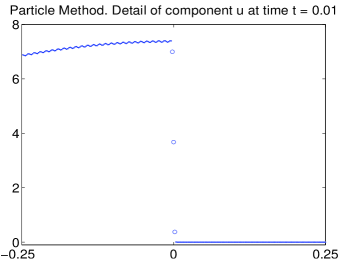
Figure 1: Experiment 1. Left panel: Exact and particle method approximation. At this scale, both are indistinguishable. Right panel: A detail of the solution showing the oscillating instabilities and the need of only three particles to covering the discontinuity of the exact solution.

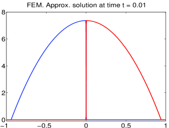
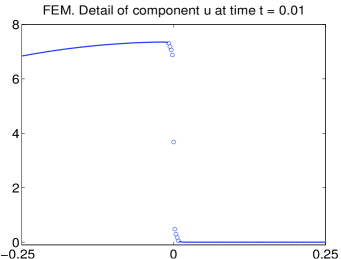
Figure 2: Experiment 1. Left panel: Exact and FEM approximation. Again, at this scale, both are indistinguishable. Right panel: A detail of the solution showing that more nodes than in the particle method are needed to cover the discontinuity of the exact solution. However, no instabilities are present.

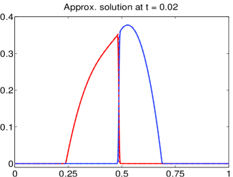
Figure 3: Experiment 2. Particle (continuous line) and FEM (dotted line) approximations. Only at the discontinuity point a difference between both approximations may be observed.

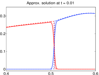
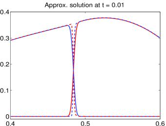
Figure 4: Experiment 2. Detail of Fig. 3 at the contact inhibition point.

References

- [1] M. Andreianov, B. Bendahmane, R. Ruiz-Baier, Analysis of a finite volume method for a cross-diffusion model in population dynamics, Math. Mod. Meth. Appl. Sci. 21(2) (2011) 307–344.
- [2] I. S. Aranson, L. S. Tsimring, Continuum theory of partially fluidized granular flows, Phys. Rev. E (3) 65 (2002) 061303.
- [3] L. A. Barba, A. Leonard, C. B. Allen, Advances in viscous vortex methods-meshless spatial adaption based on radial basis function interpolation, Int. J. Numer. Meth. Fluids 47 (2005) 387–421.
- [4] J. W. Barrett, J. F. Blowey, Finite element approximation of a nonlinear cross-diffusion population model, Numer. Math. 98 (2004) 195–221.
- [5] M. Bendahmane, Weak and classical solutions to predator-prey system with cross-diffusion, Nonlinear Anal. 73 (2010) 2489–2503.
- [6] S. Berres, R. Ruiz-Baier, A fully adaptive numerical approximation for a two-dimensional epidemic model with nonlinear cross-diffusion, Nonlinear Anal. Real World Appl. 12 (2011) 2888–2903.
- [7] M. Bertsch, M. E. Gurtin, D. Hilhorst, L. A. Peletier, On interacting populations that disperse to avoid crowding: preservation of segregation, J. Math. Biol. 23 (1985) 1–13
- [8] M. Bertsch, D. Hilhorst, H. Izuhara, M. Mimura, A nonlinear parabolic-hyperbolic system for contact inhibition of cell-growth, Diff. Equ. Appl. 4 (2012) 137–157.
- [9] S. N. Busenberg, C. C. Travis, Epidemic models with spatial spread due to population migration, J. Math. Biol. 16 (1983) 181–198.
- [10] M. Chaplain, L. Graziano, L. Preziosi, Mathematical modelling of the loss of tissue compression responsiveness and its role in solid tumour development, Math. Med. Biol. 23 (2006) 197–229.
- [11] L. Chen, A. Jüngel, Analysis of a multidimensional parabolic population model with strong cross-diffusion, SIAM J. Math. Anal. 36(1) (2004) 301–322.
- [12] L. Chen, A. Jüngel, Analysis of a parabolic cross-diffusion semiconductor model with electron-hole scattering, Comm. Partial Differential Equations, 32 (2007) 127–148.
- [13] P. Degond, S. Mas-Gallic, The weighted particle method for convection–diffusion equations. Part I. The case of an isotropic viscosity and Part II. The anisotropic case, Math. Comp. 53 (1989) 485–525.
- [14] P. Degond, F.-J. Mustieles, A deterministic approximation of diffusion equations using particles, SIAM J. Sci. Stat. Comput. 11 (1990) 293– 310.
- [15] P. Deuring, An initial-boundary value problem for a certain density-dependent diffusion system, Math. Z. 194 (1987) 375-396.
- [16] G. Galiano, On a cross-diffusion population model deduced from mutation and splitting of a single species, Comput. Math. Appl. 64(6) (2012) 1927-1936.
- [17] G. Galiano, M. L. Garzón, A. Jüngel, Analysis and numerical solution of a nonlinear cross-diffusion system arising in population dynamics, RACSAM Rev. R. Acad. Cienc. Exactas Fís. Nat. Ser. A Mat. 95(2) (2001) 281–295.
- [18] G. Galiano, M. L. Garzón, A. Jüngel, Semi-discretization in time and numerical convergence of solutions of a nonlinear cross-diffusion population model, Numer. Math. 93(4) (2003) 655–673.
- [19] G. Galiano, A. Jüngel, J. Velasco, A parabolic cross-diffusion system for granular materials, SIAM J. Math. Anal. 35(3) (2003) 561–578.
- [20] G. Galiano, V. Selgas, On a cross-diffusion segregation problem arising from a model of interacting particles. To appear in Nonlinear Anal. Real World Appl.
- [21] G. Galiano, S. Shmarev , J. Velasco, Existence and non-uniqueness of segregated solutions to a class of cross-diffusion systems. In preparation.
- [22] G. Galiano, J. Velasco, Competing through altering the environment: A cross–diffusion population model coupled to transport-darcy flow equations, Nonlinear Anal. Real World Appl. 12(5) (2011) 2826–2838.
- [23] G. Gambino, M.C. Lombardo and M. Sammartino, A velocity-diffusion method for a Lotka-Volterra system with nonlinear cross and self-diffusion, Appl. Numer. Math. 59 (2009) 1059–1074.
- [24] G. Gambino, M.C. Lombardo and M. Sammartino, Turing instability and traveling fronts for a nonlinear reaction–diffusion system with cross-diffusion Original, Math. Comput. Simul.82(6) (2012) 1112–1132.
- [25] G. Gambino, M.C. Lombardo and M. Sammartino, Pattern formation driven by cross–diffusion in a 2D domain, Nonlinear Anal. Real World Appl. 14(3) (2013) 1755–1779.
- [26] E. Gilad, J. von Hardenberg, A. Provenzale, M. Shachak, E. Meron. A mathematical model of plants as ecosystem engineers, J. Theoret. Biol. 244(4) (2007) 680–691.
- [27] M. E. Gurtin, A. C. Pipkin, On interacting populations that disperse to avoid crowding, Q. Appl. Math. 42 (1984) 87–94.
- [28] J. U. Kim, Smooth solutions to a quasi-linear system of diffusion equations for a certain population model, Nonlinear Anal. 8 (1984) 1121–1144.
- [29] P.-L. Lions, S. Mas-Gallic, Une méthode particulaire déterministe pour des équations diffusive non linéaires, C. R. Acad. Sci. Paris Sér. I Math. 332 (2001) 369–376.
- [30] Y. Lou, W. M. Ni, Y. Wu, Diffusion, self-diffusion and cross-diffusion, J. Differ. Equations 131(1) (1996) 79–131.
- [31] Y. Lou, W. M. Ni, Y. Wu, The global existence of solutions for a cross-diffusion system, Adv. Math. Beijing 25 (1996) 283-284.
- [32] R. Ruiz-Baier, C. Tian, Mathematical analysis and numerical simulation of pattern formation under cross-diffusion, Nonlinear Anal. Real World Appl. 14(1) (2013) 601–612.
- [33] J. A. Sherratt, Wavefront propagation in a competition equation with a new motility term modelling contact inhibition between cell populations, R. Soc. Lond. Proc. Ser. A Math. Phys. Eng. Sci. 456 (2000) 2365–2386.
- [34] N. Shigesada, K. Kawasaki, E. Teramoto, Spatial segregation of interacting species, J. Theor. Biol. 79 (1979) 83–99.
- [35] C. Tian, Z. Lin, M. Pedersen, Instability induced by cross-diffusion in reaction-diffusion systems, Nonlin. Anal. RWA 11 (2010) 1036–1045.
- [36] A. Yagi, Global solution to some quasilinear parabolic system in population dynamics, Nonlinear Anal. 21 (1993) 603–630.