Compressive Nonparametric Graphical Model Selection
for Time Series

Abstract

We propose a method for inferring the conditional independence graph (CIG) of a high-dimensional discrete-time Gaussian vector random process from finite-length observations. Our approach does not rely on a parametric model (such as, e.g., an autoregressive model) for the vector random process; rather, it only assumes certain spectral smoothness properties. The proposed inference scheme is compressive in that it works for sample sizes that are (much) smaller than the number of scalar process components. We provide analytical conditions for our method to correctly identify the CIG with high probability.

Index Terms— Sparsity, graphical model selection, multitask learning, nonparametric time series, LASSO.

1 Introduction

Consider a $p$-dimensional, zero-mean, stationary, Gaussian random process $\mathbf{x}[n]\in\mathbb{R}^{p}$, $n\in\mathbb{Z}$. We are interested in learning the conditional independence graph (CIG) [1, 2, 3, 4] of $\mathbf{x}[n]$ from the finite-length observation of a single process realization. We consider the high-dimensional regime, where the number of observed process samples is (much) smaller than $p$ [5, 6, 7, 8, 9, 10, 11]. In this case, consistent estimation of the CIG is possible only if structural assumptions on the vector process are made. Specifically, we will consider CIGs that are sparse in the sense of containing relatively few edges. This problem is relevant, e.g., in the analysis of the time evolution of air pollutant concentrations [1, 2] and in medical diagnostic data analysis [8].

Existing approaches to this compressive graphical model selection problem are based on parametric process models [8, 9, 12, 13], specifically on vector autoregressive (VAR) models. In this paper, we develop and analyze a nonparametric approach, which only requires the vector process to be spectrally smooth. The smoothness notion we use is quantified in terms of moments of the matrix-valued auto-covariance function (ACF) of the process. Compared to [10, 8, 9, 12, 13], our approach applies to a considerably more general class of processes including VAR processes as a special case.

Contributions:

Our main conceptual contribution resides in recognizing that the problem of inferring the sparse CIG of a Gaussian vector process is a special case of a block-sparse signal recovery problem [14, 15, 16], i.e., a multitask learning problem [17, 18]. While for the special case of a VAR process with sparse CIG, a block-sparse structure was already identified in [8], we show that a (different) block-sparse structure exists for general stationary time series. This stems from the fact that the CIG of a general stationary time series is encoded in the continuous ensemble of values of the spectral density matrix $\mathbf{S}(\theta)$, $\theta\in[0,1)$. Based on this insight, we develop a multitask LASSO [17, 19] formulation of the sparse CIG estimation problem. Our main analytical contribution is Theorem 4.1, which provides conditions for our scheme to correctly identify the CIG with high probability.

Outline:

The remainder of this paper is organized as follows. In Section 2, we introduce the problem considered. Section 3 describes our CIG inference method and Section 4 presents corresponding performance guarantees. Finally, Section 5 reports numerical results.

2 Problem Formulation

Consider a $p$-dimensional, zero-mean, stationary, real, Gaussian random process $\mathbf{x}[n]$ with (matrix-valued) ACF $\mathbf{R}[m]:=\operatorname*{E}\{\mathbf{x}[m]{\mathbf{x}}^{T}[0]\}$. The ACF is assumed summable, i.e., $\sum_{m=-\infty}^{\infty}\!{\|\mathbf{R}[m]\|}\!<\!\infty$ for some matrix norm $\|\!\cdot\!\|$. The spectral density matrix (SDM) of the process $\mathbf{x}[n]$ is defined as $\mathbf{S}(\theta)\!:=\!\sum_{m=-\infty}^{\infty}\mathbf{R}[m]\exp(-j2\pi\theta m)\in\mathbb{C}^{p\times p}$, and we assume that

$$0<A\leq\nu_{\text{min}}(\mathbf{S}(\theta))\leq\nu_{\text{max}}(\mathbf{S}(\theta))\leq B<\infty\vspace*{-1mm}$$ (1)

for all $\theta~\in[0,1)$, where $\nu_{\text{min}}(\mathbf{S}(\theta))$ and $\nu_{\text{max}}(\mathbf{S}(\theta))$ denote the smallest and largest eigenvalue of $\mathbf{S}(\theta)$, respectively. In particular, (1) implies that the matrix $\mathbf{S}(\theta)$ is nonsingular for all $\theta$. We will furthermore require the vector process $\mathbf{x}[n]$ to be such that $\mathbf{S}(\theta)$ satisfies certain smoothness properties which are expressed in terms of moments of the ACF defined as

$$\mu^{(h)}:=\sum_{m=-\infty}^{\infty}h[m]\|\mathbf{R}[m]\|_{\infty}.\vspace*{-.8mm}$$ (2)

Here, $h[m]$ is a nonnegative weight function that typically increases with $|m|$.

The CIG of the process $\mathbf{x}[n]$ is the graph $\mathcal{G}\!:=\!(V,E)$ with node set $V=[p]\!:=\!\{1,\ldots,p\}$ representing the scalar component processes $\{x_{r}[n]\}_{r\in[p]}$ and edge set $E\subseteq[p]\times[p]$, where $(k,l)\notin E$ if and only if the component processes $x_{k}[n]$ and $x_{l}[n]$ are conditionally independent given all remaining component processes $\{x_{r}[n]\}_{r\in[p]\setminus\{k,l\}}$ [1]. The neighborhood of node $r\in[p]$ is defined as $\mathcal{N}(r)\!:=\!\{r^{\prime}\in[p]\,\,|\,\,(r,r^{\prime})\in E\}$. We restrict ourselves to processes with sparse CIG $\mathcal{G}$ in the sense that

$$\max_{r\in[p]}|\mathcal{N}(r)|\leq s_{\text{max}}\ll p.\vspace*{-2mm}$$ (3)

The graphical model selection problem we consider can now be stated as the problem of inferring the CIG $\mathcal{G}$, or more precisely its edge set $E$, from the observation $\big{(}\mathbf{x}[1],\ldots,\mathbf{x}[N]\big{)}$, where $N$ is the sample size. Since $\mathbf{x}[n]$ is Gaussian with $\mathbf{S}(\theta)$ nonsingular for all $\theta\in[0,1)$, it follows from [1, 2, 20] that $(k,l)\notin E$ if and only if $\big{[}\mathbf{S}^{-1}(\theta)\big{]}_{k,l}=0$ for all $\theta\in[0,1)$. The edge set $E$ therefore corresponds to the locations of the nonzero entries of $\mathbf{S}^{-1}(\theta)$, and our graphical model selection problem amounts to determining these locations. We are interested in estimating the CIG $\mathcal{G}$ from $F$ regularly spaced samples $\{\mathbf{S}(\theta_{f})\}_{f\in[F]}$, with $\theta_{f}:=(f-1)/F$, $f\in[F]$, and $F$ large enough for the following to hold:

$$(k,l)\notin E\Longleftrightarrow\big{[}\mathbf{S}^{-1}(\theta_{f})\big{]}_{k,l}=0\mbox{\, for all }f\in[F].\vspace{-.5mm}$$ (4)

The implication from left to right in (4) follows trivially from what was said above. The implication from right to left is satisfied, e.g., for processes with all entries of $\mathbf{S}(\theta)$ being rational functions in $\exp(j\theta)$, provided that $F$ is larger than the maximum degree of the numerator polynomials of $\mathbf{S}^{-1}(\theta)$. Another sufficient condition for the implication from right to left to hold is the following.

Lemma 2.1.

Consider a $p$-dimensional, zero-mean, stationary, Gaussian process $\mathbf{x}[n]$ with CIG $\mathcal{G}$ and SDM $\mathbf{S}(\theta)$ satisfying (1). Then, if $F$ is chosen such that for every edge $(k,l)\in E$, the ACF moment $\mu^{(h_{0})}$ with $h_{0}[m]\!=\!|m|$ and the global partial coherence $\Gamma^{(k,l)}:=\int_{0}^{1}\Big{|}\big{[}\mathbf{S}^{-1}(\theta)\big{]}_{k,l}\Big{/}\sqrt{\big{[}\mathbf{S}^{-1}(\theta)\big{]}_{k,k}\big{[}\mathbf{S}^{-1}(\theta)\big{]}_{l,l}}\Big{|}d\theta$ satisfy $\mu^{(h_{0})}/(A\Gamma^{(k,l)})<F$, with $A$ as in (1), the CIG $\mathcal{G}$ is characterized by (4).

The restriction to the finite set of frequencies $\{\theta_{f}\}_{f\in[F]}$ is made for expositional convenience. The general theory developed in this paper goes through for $\theta\in[0,1)$, with our inference procedure becoming a multitask learning problem with a continuum instead of a finite number, $F$, of tasks.

3 Graphical Model Selection

Our method for inferring the CIG $\mathcal{G}$ is inspired by the approach employed in [10, 7]. We first estimate the SDM $\mathbf{S}(\theta_{f})$, $f\in[F]$, by means of a multivariate spectral estimator. Then we use this estimate to perform neighborhood regression, which yields an estimate of the support (i.e., the locations of the nonzero entries) of $\mathbf{S}^{-1}(\theta)$ and, via (4), the CIG. Neighborhood regression is performed by solving a multitask learning problem using multitask LASSO (mLASSO) [17].

With regards to the first step, it is natural to estimate $\mathbf{S}(\theta)$ using the multivariate Blackman-Tukey estimator [21]:

$$\widehat{\mathbf{S}}(\theta):=\sum_{m=-N+1}^{N-1}w[m]\widehat{\mathbf{R}}[m]\exp(-j2\pi\theta m).$$ (5)

Here, $\widehat{\mathbf{R}}[m]:=(1/N)\sum_{n=1}^{N-m}\mathbf{x}[n+m]{\mathbf{x}}^{T}[n]$ for $m\in\{0,\ldots,N-1\}$ and, by symmetry of the ACF, $\widehat{\mathbf{R}}[m]:=\widehat{\mathbf{R}}^{H}[-m]$ for $m\in\{-N+1,\ldots,-1\}$. Furthermore, the window function $w[m]$ is chosen such that $\widehat{\mathbf{S}}(\theta)$ is positive semidefinite. All window functions with nonnegative discrete-time Fourier transform are admissible [21, Sec. 2.5.2]. In the high-dimensional regime, where the number $N$ of observations is smaller than the number $p$ of nodes, the matrices $\widehat{\mathbf{S}}(\theta_{f})$ in (5) will be rank-deficient (to see this, note that each column of $\widehat{\mathbf{S}}(\theta_{f})$ is a linear combination of $\mathbf{x}[n],n\in[N]$). Simply inverting $\widehat{\mathbf{S}}(\theta_{f})$, for $f\in[F]$, and inferring the edge set $E$ via (4) is therefore not possible.

To cope with this issue, we reduce the problem of finding the support of the matrices $\mathbf{S}^{-1}(\theta_{f})$ to multitask learning problems (one for each node). This can be done as follows. First note that, because of (4), the union of the supports of the $r$th rows of the matrices $\mathbf{S}^{-1}(\theta_{f}),f\in[F]$, determines the neighborhood $\mathcal{N}(r)$. The $\mathcal{N}(r)$, as shown next, can then be obtained by solving multitask learning problems. For simplicity of exposition and without loss of generality we assume $r=1$ in the following. Given $\mathbf{S}(\theta_{f})$, $f\in[F]$, we define $\mathbf{y}^{(f)}\in\mathbb{C}^{p}$ and $\mathbf{X}^{(f)}\in\mathbb{C}^{p\times(p-1)}$ via

$$[\mathbf{y}^{(f)}\,\;\mathbf{X}^{(f)}]:=\mathbf{S}^{1/2}(\theta_{f})\vspace{-1mm}$$ (6)

where $\mathbf{S}^{1/2}(\theta_{f})$ is the positive definite square root of $\mathbf{S}(\theta_{f})$. We next decompose $\mathbf{y}^{(f)}$ into its orthogonal projection onto $\operatorname*{span}(\mathbf{X}^{(f)})$ and the orthogonal complement thereof according to

$$\mathbf{y}^{(f)}=\mathbf{X}^{(f)}\bm{\beta}^{(f)}+\bm{\varepsilon}^{(f)},\quad f\in[F]\vspace{.4mm}$$ (7)

with $\bm{\beta}^{(f)}:={\mathbf{X}^{(f)}}^{\dagger}\mathbf{y}^{(f)}$ and $\bm{\varepsilon}^{(f)}:=(\mathbf{I}-\mathbf{X}^{(f)}{\mathbf{X}^{(f)}}^{\dagger})\mathbf{y}^{(f)}$, where ${\mathbf{X}^{(f)}}^{\dagger}$ is the pseudo-inverse of $\mathbf{X}^{(f)}$. The significance of this construction is expressed by the following proposition.

Proposition 3.1.

The neighborhood $\mathcal{N}(1)$ of node $r=1$ is determined by the joint support of the $\bm{\beta}^{(f)},f\in[F]$, according to

$$\mathcal{N}(1)=\bigcup_{f\in[F]}\operatorname{supp}(\bm{\beta}^{(f)})+1\vspace{0.5mm}$$ (8)

where the addition in (8) is elementwise.

Proof.

We first note that (4) implies

$$\mathcal{N}(1)=\bigcup_{f\in[F]}\operatorname{supp}([{\mathbf{S}}^{-1}(\theta_{f})]_{2:p,1})+1\vspace{-0.2cm}$$

where $[{\mathbf{S}}^{-1}(\theta_{f})]_{2:p,1}$ is the vector containing the entries $[\mathbf{S}^{-1}(\theta_{f})]_{2,1},[\mathbf{S}^{-1}(\theta_{f})]_{3,1},...,[\mathbf{S}^{-1}(\theta_{f})]_{p,1}$. Next, we show that $\operatorname{supp}([{\mathbf{S}}^{-1}(\theta_{f})]_{2:p,1})=\operatorname{supp}(\bm{\beta}^{(f)})$, which will finalize the proof. By the construction of $\mathbf{y}^{(f)}$ and $\mathbf{X}^{(f)}$ in (6), we have

$$\mathbf{S}(\theta_{f})=\begin{bmatrix}{\|\mathbf{y}^{(f)}\|}_{2}^{2}&{\mathbf{y}^{(f)}}^{H}\mathbf{X}^{(f)}\\[5.69046pt] {\mathbf{X}^{(f)}}^{H}\mathbf{y}^{(f)}&{\mathbf{X}^{(f)}}^{H}\mathbf{X}^{(f)}\end{bmatrix}.$$ (9)

Applying a well-known formula for the inverse of a block matrix  [22, Fact 2.17.3] to $\mathbf{S}(\theta_{f})$ yields $\big{[}\mathbf{S}^{-1}(\theta_{f})\big{]}_{2:p,1}=-\omega\bm{\beta}^{(f)}$with $\omega:=\big{(}{\mathbf{y}^{(f)}}^{H}\!\bm{\varepsilon}^{(f)}\big{)}^{-1}.$ It also follows from [22, Fact 2.17.3] that $\omega=\big{[}\mathbf{S}^{-1}(\theta_{f})\big{]}_{1,1}$ and hence $\omega>0$ by (1), which allows us to conclude that $\operatorname{supp}([{\mathbf{S}}^{-1}(\theta_{f})]_{2:p,1})=\operatorname{supp}(\bm{\beta}^{(f)})$. ∎

The essence of Proposition 3.1 is that it reduces the problem of determining the neighborhood $\mathcal{N}(1)$ to that of finding the joint support of the $\bm{\beta}^{(f)},f\in[F]$. Recovering the $\bm{\beta}^{(f)}$ based on the observations (7) is now recognized as a multitask learning or generalized multiple measurement vector problem [17, 18, 23], which in turn is a special case (with additional structure) of a block-sparse signal recovery problem [14, 15, 16]. Specifically, a multi-task learning problem can be cast as a block-sparse signal recovery problem by stacking the individual linear models in (7) into a single linear model; the resulting system matrix $\operatorname*{diag}\{\mathbf{X}^{(f)}\}_{f\in[F]}$ is block-diagonal. The approach described in [8] for VAR processes, albeit leading to a block-sparse recovery problem, does not result in a block-diagonal system matrix.

An efficient method for solving the multi-task learning problem at hand is the mLASSO, which can be formulated as follows (e.g., [17]):

$$\hat{\bm{\beta}}=\operatorname*{arg\;min}_{\bm{\beta}\in\mathbb{C}^{F(p-1)}}\bigg{\{}\frac{1}{F}\sum_{f\in[F]}{\|\mathbf{y}^{(f)}-\mathbf{X}^{(f)}\bm{\beta}^{(f)}\|}_{2}^{2}+\lambda{\|\bm{\beta}\|}_{2,1}\bigg{\}}$$

where $\lambda>0$ is the LASSO parameter, $\bm{\beta}:=\big{(}{{\bm{\beta}}^{(1)}}^{T}\!\!\cdots\,\break{{\bm{\beta}}^{(F)}}^{T}\big{)}^{T}\in\mathbb{C}^{F(p-1)},$ and ${\|\bm{\beta}\|}_{2,1}:=\sum_{r\in[p-1]}{\|\bm{\beta}_{r}\|}_{2}$ with $\bm{\beta}_{r}\in\mathbb{C}^{F}$ given by $[\bm{\beta}_{r}]_{f}:=[\bm{\beta}^{(f)}]_{r}$. To compute the estimate $\hat{\bm{\beta}}$, one does not need to compute $\mathbf{y}^{(f)}$ and $\mathbf{X}^{(f)}$ by taking the square root of $\mathbf{S}(\theta_{f})$ as in (6). To see this, we note that (LABEL:equ_multitask_lasso_graph_sel_statistic) is equivalent to

$$\hat{\bm{\beta}} =\!\operatorname*{arg\;min}_{\bm{\beta}\in\mathbb{C}^{F(p-1)}}\bigg{\{}\frac{1}{F}\sum_{f\in[F]}\big{[}{{\bm{\beta}}^{(f)}}^{H}{\mathbf{X}^{(f)}}^{H}\mathbf{X}^{(f)}{\bm{\beta}}^{(f)}$$

$$\hskip 45.5244pt\!-\!2\Re\big{\{}{\mathbf{y}^{(f)}}^{H}\mathbf{X}^{(f)}{\bm{\beta}}^{(f)}\big{\}}\big{]}+\lambda{\|\bm{\beta}\|}_{2,1}\bigg{\}}$$ (11)

and, by (9), ${\mathbf{y}^{(f)}}^{H}\mathbf{X}^{(f)}$ and ${\mathbf{X}^{(f)}}^{H}\mathbf{X}^{(f)}$ are submatrices of $\mathbf{S}(\theta_{f})$. Therefore, working with (3) instead of (LABEL:equ_multitask_lasso_graph_sel_statistic) has the advantage that the square root $\mathbf{S}^{1/2}(\theta_{f})$ does not need to be computed in order to determine $\hat{\bm{\beta}}$.

In summary, we have shown that the neighborhood $\mathcal{N}(1)$ can be found via the support of the mLASSO estimate (3). Recognizing that this estimate depends on $\mathbf{S}(\theta_{f})$, which is unknown, motivates the following inference algorithm (for general $r$), which simply uses $\widehat{\mathbf{S}}(\theta_{f})$ instead of $\mathbf{S}(\theta_{f})$ in (3).

Algorithm 1.

Given the observation $\mathbf{x}[1],...,\mathbf{x}[N]$, the parameter $F$, the threshold parameter $\eta$, and the mLASSO parameter $\lambda$ (the choice of $\eta$ and $\lambda$ will be discussed in Section 4), perform the following steps:

Step 1: For each $f\in[F]$, compute the SDM estimate $\widehat{\mathbf{S}}(\theta_{f})$ according to (5).

Step 2: Compute the mLASSO estimate for each $r\in[p]$ as

$$\hat{\bm{\beta}} =\!\operatorname*{arg\;min}_{\bm{\beta}\in\mathbb{C}^{F(p-1)}}\bigg{\{}\frac{1}{F}\!\!\sum_{f\in[F]}\big{[}{{\bm{\beta}}^{(f)}}^{H}\mathbf{G}_{r}{(f)}{\bm{\beta}}^{(f)}$$

$$\hskip 45.5244pt\!-\!2\Re\big{\{}{\mathbf{c}_{r}^{(f)}}^{H}{\bm{\beta}}^{(f)}\big{\}}\big{]}+\lambda{\|\bm{\beta}\|}_{2,1}\bigg{\}}$$ (12)

where $\mathbf{G}_{r}^{(f)}\in\mathbb{C}^{(p-1)\times(p-1)}$ is the submatrix of $\widehat{\mathbf{S}}(\theta_{f})\in\mathbb{C}^{p\times p}$ obtained by deleting its $r$th column and $r$th row, and $\mathbf{c}_{r}^{(f)}\in\mathbb{C}^{(p-1)}$ is obtained by deleting the $r$th entry in the $r$th column of $\widehat{\mathbf{S}}(\theta_{f})$.

Step 3: Estimate the neighborhood of node $r$ as the index set

$$\widehat{\mathcal{N}}(r)=\big{\{}r^{\prime}\,\big{|}\,{\|\hat{\bm{\beta}}_{r^{\prime}}\|}_{2}>\eta\big{\}}$$ (13)

with $\hat{\bm{\beta}}_{r^{\prime}}\in\mathbb{C}^{F}$ given by $[\hat{\bm{\beta}}_{r^{\prime}}]_{f}=[\hat{\bm{\beta}}^{(f)}]_{r^{\prime}}$.

Our algorithm can be regarded as a generalization of the algorithm proposed in [10] for i.i.d. random processes to general stationary random processes. The new element here is that since we consider general Gaussian vector processes, we have multiple measurements available to determine the CIG. This is exploited through the use of mLASSO instead of plain LASSO as employed in [10].

4 Performance Guarantees

We now present conditions for our CIG selection scheme to correctly identify, with high probability, the neighborhoods $\mathcal{N}(r)$, and in turn the edge set $E$, of the underlying CIG. Our analysis yields allowed growth rates for the problem dimensions, i.e., the number $p$ of scalar process components and the maximum node degree $s_{\text{max}}$, as functions of the sample size $N$. Moreover, we provide concrete choices for the threshold parameter $\eta$ in (13) and the mLASSO parameter $\lambda$ in (1).

A necessary and sufficient condition for mLASSO to correctly identify the joint support of the underlying parameter vector is the incoherence condition [24, Eqs. (4)–(5)]. This condition is a worst-case (in our case, over frequency $\theta_{f}$) condition [23] in that it needs the system matrices $\{\mathbf{X}^{(f)}\}_{f\in[F]}$ in (7) (again, we consider node $r=1$) to be “well-conditioned” for all $f\in[F]$. In other words, the incoherence condition does not predict any performance improvement owing to the availability of $F$ measurements (7) instead of just one. We will therefore base our performance analysis on the multitask compatibility constant [17], which is defined, for a given index set $\mathcal{S}\subseteq[p-1]$ of size $s$, as

$$\phi(\mathcal{S}):=\min_{\bm{\beta}\in\mathbb{A}(\mathcal{S})}\frac{1}{\|\bm{\beta}_{\mathcal{S}}\|_{2,1}}\bigg{(}s\sum_{f\in[F]}{\|\mathbf{X}^{(f)}\bm{\beta}^{(f)}\|}_{2}^{2}~\bigg{)}^{1/2}\vspace*{-1mm}$$ (14)

with $\mathbb{A}(\mathcal{S})\triangleq\big{\{}\bm{\beta}\in\mathbb{C}^{(p-1)F}\big{|}\|\bm{\beta}_{\mathcal{S}}\|_{2,1}>0\mbox{ and }\|\bm{\beta}_{{\mathcal{S}}^{c}}\|_{2,1}\leq 3\|\bm{\beta}_{\mathcal{S}}\|_{2,1}\}$. Here, $\bm{\beta}_{\mathcal{S}}:=\big{(}{\bm{\beta}_{\mathcal{S}}^{(1)}}^{T}\!\!\cdots\,{\bm{\beta}_{\mathcal{S}}^{(F)}}^{T}\big{)}^{T}$ where $\bm{\beta}_{\mathcal{S}}^{(f)}$ is the restriction of the vector $\bm{\beta}^{(f)}$ to the entries in $\mathcal{S}$. Invoking the concept of the multitask compatibility constant will be seen below to yield an average (across frequency $\theta_{f}$) requirement on the SDM $\mathbf{S}(\theta_{f})$ for Algorithm 13 to correctly identify the CIG.

We start by defining the class $\mathcal{M}\!=\!\mathcal{M}(s_{\text{max}},\rho_{\text{min}},\mu^{(h_{1})},\break\phi_{\text{min}},A,B)$ of $p$-dimensional, zero-mean, stationary, Gaussian processes $\mathbf{x}[n]$ with CIG $\mathcal{G}=([p],E)$ of maximum node degree $s_{\text{max}}$ (cf. (3)) and SDM $\mathbf{S}(\theta)\in\mathbb{C}^{p\times p}$ satisfying (1) and (4). The remaining parameters characterizing this class are defined as follows:

• Minimum partial coherence $\rho_{\text{min}}>0$: This parameter quantifies the minimum partial correlation between the spectral components of the process. In particular, we require that, for every $r\in[p]$, $r^{\prime}\in\mathcal{N}(r)$,

  $$\sum_{f\in[F]}\left|\frac{\big{[}\mathbf{S}^{-1}(\theta_{f})\big{]}_{r,r^{\prime}}}{\big{[}\mathbf{S}^{-1}(\theta_{f})\big{]}_{r,r}}\right|^{2}\geq\rho^{2}_{\text{min}}.\vspace*{-3mm}$$

• ACF moment $\mu^{(h_{1})}$: We quantify the spectral smoothness of the processes in $\mathcal{M}$ using the ACF moment (2) with weight function $h_{1}[m]:=\left|1-w[m](1-|m|/N)\right|$, where $w$ is the window function in (5).

• Minimum multitask compatibility constant $\phi_{\text{min}}>0$ (cf. (14)): For every process in $\mathcal{M}$, we require

  $$\frac{1}{\|\bm{\beta}_{\mathcal{N}(r)}\|_{2,1}}\bigg{(}|\mathcal{N}(r)|\!\!\sum_{f\in[F]}{\bm{\beta}^{(f)}}^{H}\mathbf{G}_{r}^{(f)}\bm{\beta}^{(f)}\!\bigg{)}^{1/2}\geq\phi_{\text{min}}$$

  to hold for all $\bm{\beta}\in\mathbb{A}(\mathcal{N}(r))$ and all $r\in[p]$.

Combining techniques from large deviation theory [25] to bound the error $\|\widehat{\mathbf{S}}(\theta_{f})-\mathbf{S}(\theta_{f})\|_{\infty}$ with a deterministic performance analysis of the mLASSO [17], one can derive the following result.

Theorem 4.1.

Consider a process $\mathbf{x}[n]$ belonging to the class $\mathcal{M}$. Let $\widehat{\mathcal{N}}(r)$ be the estimate of $\mathcal{N}(r)$ given by (13), based on sample size $N$ and with the choices $\lambda=\phi_{\emph{min}}^{2}\rho_{\emph{min}}/(18s_{\emph{max}}F)$ (in (1)) and $\eta=\rho_{\emph{min}}/2$ (in (13)). Then, if for some $\delta>0$, the sample size $N$ and the ACF moment $\mu^{(h_{1})}$ satisfy

$$N>2^{8}\log\bigg{(}\frac{4Fp^{3}}{\delta}\bigg{)}\frac{\|w\|_{1}^{2}B^{2}s^{3}_{\emph{max}}}{\kappa^{2}}\mbox{\; and \;}\mu^{(h_{1})}\!\leq\!\frac{\kappa}{2s^{3/2}_{\emph{max}}}$$

with $\kappa:=(\phi_{\emph{min}}^{2}/174)\frac{\rho_{\emph{min}}}{\sqrt{F}}\sqrt{A/B}$, the probability of Algorithm 1 delivering the correct edge set $E$ is at least $1-\delta$, i.e., ${\rm P}\big{\{}\bigcap_{r\in[p]}\{\widehat{\mathcal{N}}(r)=\mathcal{N}(r)\}\big{\}}\geq 1-\delta$.

Theorem 4.1 shows that success is guaranteed with high probability if the sample size $N$ scales logarithmically in $p$ and polynomially in $s_{\text{max}}$, and if the process is sufficiently smooth, i.e., $\mu^{(h_{1})}$ is sufficiently small.

Let us particularize Theorem 4.1 to the special case of a VAR(1) process $\mathbf{x}[n]$ as considered in [9, 13, 12], i.e., $\mathbf{x}[n]=\mathbf{A}\mathbf{x}[n-1]+\mathbf{w}[n]$ with i.i.d. noise $\mathbf{w}[n]~\sim\mathcal{N}(\mathbf{0},\sigma^{2}\mathbf{I})$. As in [9], we take $\mathbf{A}$ to be the adjacency matrix of a dependency graph $\mathcal{D}$, which is related to—but in general different from—the CIG $\mathcal{G}$. We assume that $\mathcal{D}$ is a simple graph of maximum node degree $d_{\text{max}}$ and the nonzero entries of the adjacency matrix are all equal to a single positive number $a\leq 1/(2d_{\text{max}})$. The VAR(1) process we consider satisfies (1) and (3) by its definition and belongs to the class $\mathcal{M}(s_{\text{max}},\rho_{\text{min}},\mu^{(h_{1})},\phi_{\text{min}},A,B)$ with $s_{\text{max}}=d_{\text{max}}^{2}$, $\rho_{\text{min}}=a$, $\phi_{\text{min}}=\sigma^{2}/4$, $A=\sigma^{2}/4$, and $B=4\sigma^{2}$. Moreover, condition (4) is satisfied as soon as $F\geq 3$ since the entries of $\mathbf{S}^{-1}(\theta)$ are rational functions in $\exp(j\theta)$ with numerator degree $2$. The threshold in (LABEL:eq:condonN) becomes $N>C_{1}\log\big{(}\frac{4Fp^{3}}{\delta}\big{)}\|w\|_{1}^{2}Fd^{6}_{\text{max}}/a^{2}$, with a constant $C_{1}$ that is independent of $\delta$, $p$, $d_{\text{max}}$, and $a$. In contrast, the corresponding threshold for the method in [9] is $N>C_{2}\log\big{(}\frac{4d_{\text{max}}p^{2}}{\delta}\big{)}d_{\text{max}}^{3}/a^{2}$, with a constant $C_{2}$ that is independent of $\delta$, $p$, $d_{\text{max}}$, and $a$. The difference between the growth rates of these thresholds with respect to $d_{\text{max}}$ may be explained by the fact that the method in [9] is tailored to VAR processes whereas our approach applies to general (spectrally smooth) stationary processes.

5 Numerical Results

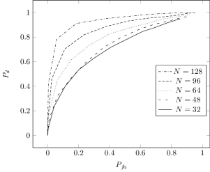
Fig. 1: ROC curves for the compressive selection scheme.

We generated a Gaussian process $\mathbf{x}[n]$ of dimension $p=64$ by applying a finite impulse response (FIR) filter $g[m]$ of length $2$ to a zero-mean, stationary, white, Gaussian noise process $\mathbf{e}[n]\sim\mathcal{N}(\mathbf{0},\mathbf{C}_{0})$. The covariance matrix $\mathbf{C}_{0}$ was chosen such that the resulting CIG $\mathcal{G}=([p],E)$ satisfies (3) with $s_{\text{max}}=3$. The filter coefficients $g[m]$ are such that the magnitude of the associated transfer function is uniformly bounded from above and below by positive constants, thereby ensuring that conditions (1) and (4) (for arbitrary $F$) are satisfied. We then computed the estimates $\widehat{\mathcal{N}}(r)$ using Algorithm 13 with window function $w[m]=\exp(-m^{2}/44)$ and $F=4$. We set $\lambda=c_{1}\phi^{2}_{\text{min}}\rho_{\text{min}}/(18s_{\text{max}}F)$ and $\eta=\rho_{\text{min}}/2$, where $\phi_{\text{min}}=0.0616$, $\rho_{\text{min}}=0.5$, and $c_{1}$ was varied in the range $[10^{-3},10^{3}]$.

In Fig. 1, we show receiver operating characteristic (ROC) curves with the average fraction of false alarms $P_{f\!a}:=\frac{1}{M}\sum_{i\in[M]}\frac{\sum_{(r,r^{\prime})\notin E}I(r^{\prime}\in\widehat{\mathcal{N}}_{i}(r))}{p(p-1)/2-|E|}$ and the average fraction of correct decisions $P_{d}:=\frac{1}{M}\sum_{i\in[M]}\frac{\sum_{(r,r^{\prime})\in E}I(r^{\prime}\in\widehat{\mathcal{N}}_{i}(r))}{|E|}$ for varying mLASSO parameter $\lambda$. Here, $\widehat{\mathcal{N}}_{i}(r)$ denotes the neighborhood estimate obtained from Algorithm 13 in the $i$-th simulation run. We averaged over $M=10$ independent simulation runs.

References

- [1] R. Dahlhaus, “Graphical interaction models for multivariate time series,” Metrika, vol. 51, pp. 151–172, 2000.
- [2] R. Dahlhaus and M. Eichler, “Causality and graphical models for time series,” in Highly Structured Stochastic Systems, P. Green, N. Hjort, and S. Richardson, Eds., pp. 115–137. Oxford Univ. Press, Oxford, UK, 2003.
- [3] F. R. Bach and M. I. Jordan, “Learning graphical models for stationary time series,” IEEE Trans. Signal Processing, vol. 52, no. 8, pp. 2189–2199, Aug. 2004.
- [4] M. Eichler, Graphical Models in Time Series Analysis, Ph.D. thesis, Universität Heidelberg, Germany, 1999.
- [5] N. E. Karoui, “Operator norm consistent estimation of large dimensional sparse covariance matrices,” Ann. Statist., vol. 36, no. 6, pp. 2717–2756, 2008.
- [6] N. P. Santhanam and M. J. Wainwright, “Information-theoretic limits of selecting binary graphical models in high dimensions,” IEEE Trans. Inf. Theory, vol. 58, no. 7, pp. 4117–4134, Jul. 2012.
- [7] P. Ravikumar, M. J. Wainwright, and J. Lafferty, “High-dimensional Ising model selection using -regularized logistic regression,” Ann. Stat., vol. 38, no. 3, pp. 1287–1319, 2010.
- [8] A. Bolstad, B. D. Van Veen, and R. Nowak, “Causal network inference via group sparse regularization,” IEEE Trans. Signal Processing, vol. 59, no. 6, pp. 2628–2641, Jun. 2011.
- [9] J. Bento, M. Ibrahimi, and A. Montanari, “Learning networks of stochastic differential equations,” in Proc. Advances in Neural Information Processing Systems, pp. 172–180, 2010.
- [10] N. Meinshausen and P. Bühlmann, “High dimensional graphs and variable selection with the Lasso,” Ann. Stat., vol. 34, no. 3, pp. 1436–1462, 2006.
- [11] J. H. Friedmann, T. Hastie, and R. Tibshirani, “Sparse inverse covariance estimation with the graphical Lasso,” Biostatistics, vol. 9, no. 3, pp. 432–441, Jul. 2008.
- [12] J. Songsiri, J. Dahl, and L. Vandenberghe, “Graphical models of autoregressive processes,” in Convex Optimization in Signal Processing and Communications, Y. C. Eldar and D. Palomar, Eds., pp. 89–116. Cambridge Univ. Press, Cambridge, UK, 2010.
- [13] J. Songsiri and L. Vandenberghe, “Topology selection in graphical models of autoregressive processes,” J. Mach. Learn. Res., vol. 11, pp. 2671–2705, 2010.
- [14] Y. C. Eldar, P. Kuppinger, and H. Bölcskei, “Block-sparse signals: Uncertainty relations and efficient recovery,” IEEE Trans. Signal Processing, vol. 58, no. 6, pp. 3042–3054, June 2010.
- [15] M. Mishali and Y. C. Eldar, “Reduce and boost: Recovering arbitrary sets of jointly sparse vectors,” IEEE Trans. Signal Processing, vol. 56, no. 10, pp. 4692–4702, Oct. 2008.
- [16] Y. C. Eldar and H. Rauhut, “Average case analysis of multichannel sparse recovery using convex relaxation,” IEEE Trans. Inf. Theory, vol. 56, no. 1, pp. 505–519, Jan. 2009.
- [17] P. Bühlmann and S. van de Geer, Statistics for High-Dimensional Data, Springer, New York, 2011.
- [18] K. Lounici, M. Pontil, A. B. Tsybakov, and S. van de Geer, “Taking advantage of sparsity in multi-task learning,” in Proc. 22nd Annual Conference on Learning Theory, pp. 73–82, 2009.
- [19] S. Lee, J. Zhu, and E. P. Xing, “Adaptive multi-task Lasso: With application to eQTL detection,” in Proc. Advances in Neural Information Processing Systems, pp. 1306–1314, 2010.
- [20] R. Brillinger, “Remarks concerning graphical models for time series and point processes,” Revista de Econometria, vol. 16, pp. 1–23, 1996.
- [21] P. Stoica and R. Moses, Introduction to Spectral Analysis, Prentice Hall, Englewood Cliffs, NJ, 1997.
- [22] D. S. Bernstein, Matrix Mathematics: Theory, Facts, and Formulas, Princeton Univ. Press, Princeton, NJ, 2nd edition, 2009.
- [23] R. Heckel and H. Bölcskei, “Joint sparsity with different measurement matrices,” in Proc. 50th Allerton Conf. Commun., Control, and Comput., pp. 698–702, 2012.
- [24] F. R. Bach, “Consistency of the group Lasso and multiple kernel learning,” J. Mach. Learn. Res., vol. 9, pp. 1179–1225, 2008.
- [25] S. Foucart and H. Rauhut, A Mathematical Introduction to Compressive Sensing, Springer, New York, 2012.