Impact of a circularly polarized cavity photon field
on the charge and spin flow through an Aharonov-Casher ring

Abstract

We explore the influence of a circularly polarized cavity photon field on the transport properties of a finite-width ring, in which the electrons are subject to spin-orbit and Coulomb interaction. The quantum ring is embedded in an electromagnetic cavity and described by “exact” numerical diagonalization. We study the case that the cavity photon field is circularly polarized and compare it to the linearly polarized case. The quantum device is moreover coupled to external, electrically biased leads. The time propagation in the transient regime is described by a non-Markovian generalized master equation. We find that the spin polarization and spin photocurrents of the quantum ring are largest for circularly polarized photon field and destructive Aharonov-Casher (AC) phase interference. The charge current suppression dip due to the destructive AC phase becomes threefold under the circularly polarized photon field as the interaction of the electrons’ angular momentum and spin angular momentum of light causes many-body level splitting leading to three many-body level crossing locations instead of one. The circular charge current inside the ring, which is induced by the circularly polarized photon field, is found to be suppressed in a much wider range around the destructive AC phase than the lead-device-lead charge current. The charge current can be directed through one of the two ring arms with the help of the circularly polarized photon field, but is superimposed by vortices of smaller scale. Unlike the charge photocurrent, the flow direction of the spin photocurrent is found to be independent of the handedness of the circularly polarized photon field.

1 Introduction

Quantum rings are interferometers with unique properties owing to their rotational symmetric geometry. Because of their non-trivially connected topology, a variety of geometrical phases can be observed [1, 2, 3, 4], which can be tuned via the magnetic flux through the ring in case of the Aharonov-Bohm (AB) phase, or the strength of the spin-orbit interaction (SOI) in case of the Aharonov-Casher (AC) phase. Furthermore, the rotational symmetry of the ring resembles the characteristics of a circularly polarized photon field suggesting a strong light-matter interaction between single photons and the ring electrons. Circularly polarized light emission [5] and absorption [6] has been studied for quantum rings. Moreover, circularly polarized light has been used to generate persistent charge currents in quantum wells [7] and quantum rings [8, 9, 10, 11]. The basic principle behind this is a change of the orbital angular momentum of the electrons in the quantum ring by the absorption or emission of a photon leading to the circular charge transport. We would like to mention that one can improve over circularly polarized light to achieve optimal optical control for a finite-width quantum ring [12]. Rather than trying to optimize quantum transitions, we are focusing here on various interesting effects that a circularly polarized photon field has on quantum rings of spin-orbit and Coulomb interacting electrons.

The transport properties of magnetic-flux threaded rings, which are connected to two leads have been investigated in detail [13, 14]. The conductance of the ring shows characteristic oscillations with period $\Phi_{0}=hc/e$, called AB oscillations, which were measured for the first time in 1985 [15]. The electrons’ spin is not only interacting with a magnetic field via the Zeeman interaction, but also with an electric field via a so-called effective magnetic field stemming from special relativity [16]. The interaction between the spin and the electronic motion in, for example, the electric field, is called the Rashba SOI [17], which leads to the AC effect. Experimentally, the strength of the Rashba interaction can be varied by changing the magnitude of the electric field when it is oriented parallel to the central axis of the quantum ring. Another type of SOI is the Dresselhaus interaction [18], leading to the AC effect as well. The combined effects of SOI and an applied magnetic field on the electronic transport through quantum rings connected to leads have been addressed in several studies [19, 20, 21, 22, 23]. In this work, we use a small magnetic field outside the AB regime and a tunable Rashba or Dresselhaus SOI up to a strength corresponding to an AC phase difference $\Delta\Phi\approx 3\pi$ and use cavity quantum electrodynamics to describe the interaction of the electronic system with a circularly polarized photon field in a cavity.

While the magnetic flux through the ring causes only equilibrium persistent charge currents [24, 25], SOI can also induce equilibrium persistent spin currents [26, 27]. Dynamical spin currents can be obtained by two asymmetric electromagnetic pulses [28]. Optical control of the spin current can be achieved by a non-adiabatic, two-component laser pulse [29]. The persistent spin current is in general not conserved [30]. Proposals to measure persistent spin currents by the induced mechanical torque [31] or the induced electric field [30] exist.

Quantum systems embedded in an electromagnetic cavity have become one of the most promising devices for quantum information processing applications [32, 33, 34]. We are considering here the influence of the cavity photons on the spin polarization of the quantum ring and on the transient charge and spin transport inside and into and out of the ring. We treat the electron-photon interaction by using exact numerical diagonalization including many levels [35], i.e. beyond a two-level Jaynes-Cummings model or the rotating wave approximation and higher order corrections of it [36, 37, 38]. The electronic transport through a quantum system that is strongly coupled to leads has been investigated for linearly polarized electromagnetic fields [39, 40, 41, 42, 43]. For a weak coupling between the system and the leads, the Markovian approximation, which neglects memory effects in the system, can be used [44, 45, 46, 47]. To describe a stronger transient system-lead coupling, we use a non-Markovian generalized master equation [48, 49, 50] in a time-convolutionless form [51, 52], which involves energy-dependent coupling elements. We used this type of master equations earlier to explore the interplay of linearly polarized cavity photons and topological phases of quantum rings for the AB [52] and AC [53] phase. The influence of a quantized cavity photon mode of circularly polarized light on the time-dependent transport of spin-orbit and Coulomb interacting electrons under non-equilibrium conditions through a topologically nontrivial broad ring geometry, which is connected to leads has not yet been explored beyond the Markovian approximation. We note that we can compare our results to the analytic results for a one-dimensional quantum ring with Rashba or Dresselhaus SOI [53].

The paper is organized as follows. In Sec. 2, we describe the Hamiltonian for the central quantum ring system including SOI, which is embedded in a photon cavity and our time-dependent generalized master equation formalism for the transient coupling to semi-infinite leads. In addition, various transport quantities that are shown in Secs. 3 and 4, are here defined. Sec. 3 shows the numerical results concerning the spin polarization of the quantum ring, both for linear and for circular polarization. Sec. 4 is devoted to the transport of charge and spin. First, the non-local currents (lead-ring currents) between the leads and the system are discussed. Second, the change of the local currents inside the quantum ring due to the photon cavity (photocurrent) is considered. Finally, conclusions will be drawn in Sec. 5.

2 Theory, model and definitions

Here, we describe the Hamiltonian of the central system including the potential used to model the quantum ring, the Hamiltonian for the leads and the time evolution of the whole system described by a non-Markovian master equation. Furthermore, we define various quantities describing the transient charge and spin transport and their accumulation in the quantum ring. and the parameters used for the numerical results.

2.1 Central system Hamiltonian

The time-evolution of the closed many-body (MB) system composed of the interacting electrons and photons relative to the initial time $t=0$,

$$\hat{U}_{S}(t)=\exp\left(-\frac{i}{\hbar}\hat{H}_{S}t\right),$$ (1)

is governed by the MB system Hamiltonian

$$\hat{H}_{S} = \int d^{2}r\;\hat{\mathbf{\Psi}}^{\dagger}(\mathbf{r})\left[\left(\frac{\hat{\mathbf{p}}^{2}}{2m^{*}}+V_{S}(\mathbf{r})\right)+H_{Z}\right.$$ (2)

$$+\left.\hat{H}_{R}(\mathbf{r})+\hat{H}_{D}(\mathbf{r})\right]\hat{\mathbf{\Psi}}(\mathbf{r})+\hat{H}_{ee}+\hbar\omega\hat{a}^{\dagger}\hat{a},$$

with the spinor

$$\hat{\mathbf{\Psi}}(\mathbf{r})=\left(\begin{array}[]{c}\hat{\Psi}(\uparrow,\mathbf{r})\\ \hat{\Psi}(\downarrow,\mathbf{r})\end{array}\right)$$ (3)

and

$$\hat{\mathbf{\Psi}}^{\dagger}(\mathbf{r})=\left(\begin{array}[]{cc}\hat{\Psi}^{\dagger}(\uparrow,\mathbf{r}),&\hat{\Psi}^{\dagger}(\downarrow,\mathbf{r})\end{array}\right),$$ (4)

where

$$\hat{\Psi}(x)=\sum_{a}\psi_{a}^{S}(x)\hat{C}_{a}$$ (5)

is the field operator with $x\equiv(\mathbf{r},\sigma)$, $\sigma\in\{\uparrow,\downarrow\}$ and the annihilation operator, $\hat{C}_{a}$, for the single-electron state (SES) $\psi_{a}^{S}(x)$ in the central system. The SES $\psi_{a}^{S}(x)$ is the eigenstate labeled by $a$ of the Hamiltonian $\hat{H}_{S}-\hat{H}_{ee}-\hbar\omega\hat{a}^{\dagger}\hat{a}$ when we set the photonic part of the vector potential $\hat{\mathbf{A}}^{\mathrm{ph}}(\mathbf{r})$ in the momentum operator,

$$\hat{\mathbf{p}}(\mathbf{r})=\left(\begin{array}[]{c}\hat{p}_{x}(\mathbf{r})\\ \hat{p}_{y}(\mathbf{r})\end{array}\right)=\frac{\hbar}{i}\nabla+\frac{e}{c}\left[\mathbf{A}(\mathbf{r})+\hat{\mathbf{A}}^{\mathrm{ph}}(\mathbf{r})\right],$$ (6)

to zero. The Hamiltonian in Eq. (2) includes a kinetic part, a static external magnetic field $\mathbf{B}=B\hat{\mbox{\boldmath$z$}}$, in Landau gauge being represented by the vector potential $\mathbf{A}(\mathbf{r})=-By\mathbf{e}_{x}$ and a photon field. Furthermore, in Eq. (2),

$$H_{Z}=\frac{\mu_{B}g_{S}B}{2}\sigma_{z}$$ (7)

describes the Zeeman interaction between the spin and the magnetic field, where $g_{S}$ is the electron spin g-factor and $\mu_{B}=e\hbar/(2m_{e}c)$ is the Bohr magneton. The interaction between the spin and the orbital motion is described by the Rashba part

$$\hat{H}_{R}(\mathbf{r})=\frac{\alpha}{\hbar}\left(\sigma_{x}\hat{p}_{y}(\mathbf{r})-\sigma_{y}\hat{p}_{x}(\mathbf{r})\right)$$ (8)

with the Rashba coefficient $\alpha$ and Dresselhaus part

$$\hat{H}_{D}(\mathbf{r})=\frac{\beta}{\hbar}\left(\sigma_{x}\hat{p}_{x}(\mathbf{r})-\sigma_{y}\hat{p}_{y}(\mathbf{r})\right)$$ (9)

with the Dresselhaus coefficient $\beta$. In Eqs. (7-9), $\sigma_{x}$, $\sigma_{y}$ and $\sigma_{z}$ represent the spin Pauli matrices.

Equation (2) includes the electron-electron interaction

$$\hat{H}_{ee}=\frac{e^{2}}{2\kappa}\int dx^{\prime}\;\int dx\;\frac{\hat{\Psi}^{\dagger}(x)\hat{\Psi}^{\dagger}(x^{\prime})\hat{\Psi}(x^{\prime})\hat{\Psi}(x)}{\sqrt{|\mathbf{r}-\mathbf{r^{\prime}}|^{2}+\eta^{2}}}$$ (10)

with $e>0$ being the magnitude of the electron charge, which is treated numerically exactly. Only for numerical reasons, we include a small regularization parameter $\eta=0.2387$ nm in Eq. (10). The last term in Eq. (2) indicates the quantized photon field, where $\hat{a}^{\dagger}$ is the photon creation operator and $\hbar\omega$ is the photon excitation energy. The photon field interacts with the electron system via the vector potential

$$\hat{\mathbf{A}}^{\mathrm{ph}}=A(\mathbf{e}\hat{a}+\mathbf{e}^{*}\hat{a}^{\dagger})$$ (11)

with

$$\mathbf{e}=\left\{\begin{array}[]{cl}\mathbf{e}_{x},&\mathrm{TE}_{011}\\ \mathbf{e}_{y},&\mathrm{TE}_{101}\\ \frac{1}{\sqrt{2}}\left[\mathbf{e}_{x}+i\mathbf{e}_{y}\right],&\textrm{RH circular}\\ \frac{1}{\sqrt{2}}\left[\mathbf{e}_{x}-i\mathbf{e}_{y}\right],&\textrm{LH circular}\end{array}\right.$$ (12)

for a longitudinally-polarized ($x$-polarized) photon field ($\mathrm{TE}_{011}$), transversely-polarized ($y$-polarized) photon field ($\mathrm{TE}_{101}$), right-hand (RH) or left-hand (LH) circularly polarized photon field. The electron-photon coupling constant $g^{EM}=eAa_{w}\Omega_{w}/c$ scales with the amplitude $A$ of the electromagnetic field. It is interesting to note that the photon field couples directly to the spin via Eqs. (8), (9) and (6). For reasons of comparison and to determine the photocurrents, we also consider results without photons in the system. In this case, $\hat{\mathbf{A}}^{\mathrm{ph}}(\mathbf{r})$ and $\hbar\omega\hat{a}^{\dagger}\hat{a}$ drop out from the MB system Hamiltonian in Eq. (2). Our model of a photon cavity can be realized experimentally [32, 33, 54] by letting the photon cavity be much larger than the quantum ring (this assumption is used in the derivation of the vector potential, Eq. (11)).

2.2 Quantum ring potential

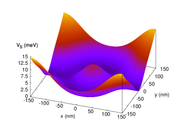
Figure 1: (Color online) System potential $V_{S}(\mathbf{r})$ of the central ring system connected to the left and right leads.

The quantum ring is embedded in the central system of length $L_{x}=300$ nm situated between two contact areas that will be coupled to the external leads, as is depicted in Fig. 1. The system potential is described by

$$V_{S}(\mathbf{r}) = \sum_{i=1}^{6}V_{i}\exp\left[-\left(\beta_{xi}(x-x_{0i})\right)^{2}-\left(\beta_{yi}y\right)^{2}\right]$$ (13)

$$+\frac{1}{2}m^{*}\Omega_{0}^{2}y^{2},$$

with the parameters from Table 1. $x_{03}=\epsilon$ is a small numerical symmetry breaking parameter and $|\epsilon|=10^{-5}$ nm is enough for numerical stability. In Eq. (13), $\hbar\Omega_{0}=1.0$ meV is the characteristic energy of the confinement in the system.

Table 1: Parameters of the ring potential in the central region.

$i$	$V_{i}$ in meV	$\beta_{xi}$ in $\frac{1}{\mathrm{nm}}$	$x_{0i}$ in nm	$\beta_{yi}$ in $\frac{1}{\mathrm{nm}}$
1	10	0.013	150	0
2	10	0.013	-150	0
3	11.1	0.0165	$\epsilon$	0.0165
4	-4.7	0.02	149	0.02
5	-4.7	0.02	-149	0.02
6	-5.33	0	0	0

2.3 Lead Hamiltonian

The Hamiltonian for the semi-infinite lead $l\in\{L,R\}$ (left or right lead),

$$\hat{H}_{l} = \int d^{2}r\;\int d^{2}r^{\prime}\;\hat{\mathbf{\Psi}}_{l}^{\dagger}(\mathbf{r}^{\prime})\delta(\mathbf{r}^{\prime}-\mathbf{r})\left[\left(\frac{\hat{\mathbf{p}}_{l}^{2}}{2m^{*}}+V_{l}(\mathbf{r})\right)\right.$$ (14)

$$+\left.H_{Z}+\hat{H}_{R}(\mathbf{r})+\hat{H}_{D}(\mathbf{r})\right]\hat{\mathbf{\Psi}}_{l}(\mathbf{r}),$$

with the momentum operator containing the kinetic momentum and the vector potential leading only to the magnetic field (i.e. not to the photon field)

$$\hat{\mathbf{p}}_{l}(\mathbf{r})=\frac{\hbar}{i}\nabla+\frac{e}{c}\mathbf{A}(\mathbf{r}).$$ (15)

We remind the reader that the Rashba part, $\hat{H}_{R}(\mathbf{r})$, (Eq. (8)) and Dresselhaus part, $\hat{H}_{D}(\mathbf{r})$, (Eq. (9)) of the SOI are momentum-dependent. For the leads, the momentum from Eq. (15), is used for the Rashba and Dresselhaus terms in Eq. (14). Equation (14) contains the lead field operator

$$\hat{\Psi}_{l}(x)=\sum_{q}\psi_{ql}(x)\hat{C}_{ql}$$ (16)

in the spinor

$$\hat{\mathbf{\Psi}}_{l}(\mathbf{r})=\left(\begin{array}[]{c}\hat{\Psi}_{l}(\uparrow,\mathbf{r})\\ \hat{\Psi}_{l}(\downarrow,\mathbf{r})\end{array}\right)$$ (17)

and a corresponding definition to Eq. (4) for the Hermitian conjugate of $\hat{\mathbf{\Psi}}_{l}(\mathbf{r})$ in Eq. (17). In Eq. (16), $\psi_{ql}(x)$ is a SES in the lead $l$ (eigenstate with quantum number $q$ of the Hamiltonian of Eq. (14)) and $\hat{C}_{ql}$ is the associated electron annihilation operator. The lead potential

$$V_{l}(\mathbf{r})=\frac{1}{2}m^{*}\Omega_{l}^{2}y^{2}$$ (18)

confines the electrons parabolically in $y$-direction in the leads with the characteristic energy $\hbar\Omega_{l}=2.0$ meV.

2.4 Time-convolutionless generalized master equation approach

We use the time-convolutionless generalized master equation [51] (TCL-GME), which is a non-Markovian master equation that is local in time. This master equation satisfies the positivity conditions [55] for the MB state occupation probabilities in the reduced density operator (RDO) usually to a relatively strong system-lead coupling [52]. We assume the initial total statistical density matrix to be a product state of the system and leads density matrices, before we switch on the coupling to the leads,

$$\hat{W}(0)=\hat{\rho}_{L}\otimes\hat{\rho}_{R}\otimes\hat{\rho}_{S}(0),$$ (19)

with $\rho_{l}$, $l\in\{L,R\}$, being the normalized density matrices of the leads. The coupling Hamiltonian between the central system and the leads reads

$$\hat{H}_{T}(t)=\sum_{l=L,R}\int dq\;\chi^{l}(t)\left[\hat{\mathfrak{T}}^{l}(q)\hat{C}_{ql}+\hat{C}_{ql}^{\dagger}\hat{\mathfrak{T}}^{l\dagger}(q)\right]\,.$$ (20)

The coupling is switched on at $t=0$ via the switching function

$$\chi^{l}(t)=1-\frac{2}{e^{\alpha^{l}t}+1}$$ (21)

with a switching parameter $\alpha^{l}$ and

$$\hat{\mathfrak{T}}^{l}(q)=\sum_{\alpha\beta}|\alpha)(\beta|\sum_{a}T_{qa}^{l}(\alpha|\hat{C}_{a}^{\dagger}|\beta).$$ (22)

Equation (22) is written in the MB eigenbasis $\{|\alpha)\}$ of the system Hamiltonian, Eq. (2). The coupling tensor [56]

$$T_{qa}^{l} = \sum_{\sigma}\sum_{\sigma^{\prime}}\int_{\Omega^{l}}d^{2}r\;\int_{\Omega_{S}^{l}}d^{2}r^{\prime}\;\psi_{ql}^{*}(\mathbf{r},\sigma)$$ (23)

$$\times g_{aq}^{l}(\mathbf{r},\mathbf{r^{\prime}},\sigma,\sigma^{\prime})\psi_{a}^{S}(\mathbf{r}^{\prime},\sigma^{\prime})$$

couples the lead SES $\{\psi_{ql}(\mathbf{r},\sigma)\}$ with energy spectrum $\{\epsilon^{l}(q)\}$ to the system SES $\{\psi_{a}^{S}(\mathbf{r},\sigma)\}$ with energy spectrum $\{E_{a}\}$ that reach into the contact regions [57], $\Omega_{S}^{l}$ and $\Omega_{l}$, of system and lead $l$, respectively, and the coupling kernel

$$g_{aq}^{l}(\mathbf{r},\mathbf{r^{\prime}},\sigma,\sigma^{\prime}) = g_{0}^{l}\delta_{\sigma,\sigma^{\prime}}\exp\left[-\delta_{x}^{l}(x-x^{\prime})^{2}\right]$$ (24)

$$\times\exp\left[-\delta_{y}^{l}(y-y^{\prime})^{2}\right]$$

$$\times\exp{\left(-\frac{|E_{a}-\epsilon^{l}(q)|}{\Delta^{l}_{E}}\right)}$$

suppresses different-spin coupling. Note that the meaning of $x$ in Eq. (24) is $\mathbf{r}=(x,y)$ and not $x=(\mathbf{r},\sigma)$. In Eq. (24), $g_{0}^{l}$ is the lead coupling strength and $\delta^{l}_{x}$ and $\delta^{l}_{y}$ are the contact region parameters for lead $l$ in $x$- and $y$-direction, respectively. Moreover, $\Delta^{l}_{E}$ denotes the affinity constant between the central system SES energy levels $\{E_{a}\}$ and the lead energy levels $\{\epsilon^{l}(q)\}$.

When propagated with the TCL-GME [51, 52], the RDO of the system,

$$\hat{\rho}_{S}(t)=\mathrm{Tr}_{L}\mathrm{Tr}_{R}[\hat{W}(t)],$$ (25)

evolves to second order in the lead coupling strength via

$$\dot{\hat{\rho}}_{S}(t) = -\frac{i}{\hbar}[\hat{H}_{S},\hat{\rho}_{S}(t)]$$ (26)

$$-\Bigg{[}\sum_{l=L,R}\int dq\;\Big{[}\hat{\mathfrak{T}}^{l}(q),\hat{\Omega}^{l}(q,t)\hat{\rho}_{S}(t)$$

$$-f(\epsilon^{l}(q))\left\{\hat{\rho}_{S}(t),\hat{\Omega}^{l}(q,t)\right\}\Big{]}+\mathrm{H.c.}\Bigg{]}$$

with the Fermi distribution function $f(E)$,

$$\hat{\Omega}^{l}(q,t) = \frac{1}{\hbar^{2}}\chi^{l}(t)\exp\left(-\frac{i}{\hbar}t\epsilon^{l}(q)\right)$$ (27)

$$\times\hat{U}_{S}(t)\hat{\Pi}^{l}(q,t)\hat{U}_{S}^{\dagger}(t)$$

and

$$\hat{\Pi}^{l}(q,t) = \int_{0}^{t}dt^{\prime}\;\left[\exp\left(\frac{i}{\hbar}t^{\prime}\epsilon^{l}(q)\right)\chi^{l}(t^{\prime})\right.$$ (28)

$$\times\left.\hat{U}_{S}^{\dagger}(t^{\prime})\hat{\mathfrak{T}}^{l\dagger}(q)\hat{U}_{S}(t^{\prime})\right].$$

2.5 Transport quantities used in the numerical results

We investigate numerically the non-equilibrium electron transport properties through a quantum ring system, which is situated in a photon cavity and weakly coupled to leads for the parameters given in the A. To explore the influence of the circularly polarized photon field and Rashba and Dresselhaus coupling on the non-local charge and spin polarization current from and into the leads, we define the non-local right-going charge current $I_{l}^{c}(t)$ (lead-ring charge current) in lead $l=L,R$ by

$$I_{l}^{c}(t)=c_{l}\mathrm{Tr}[\dot{\hat{\rho}}_{S}^{l}(t)\hat{Q}]$$ (29)

with $c_{L}=1$ and $c_{R}=-1$, with the charge operator

$$\hat{Q}=\int d^{2}r\;\hat{n}^{c}(\mathbf{r})$$ (30)

and the time-derivative of the RDO in the MB basis due to the coupling to the lead $l\in\{L,R\}$

$$\dot{\hat{\rho}}_{S}^{l}(t) = -\int dq\;\Big{[}\mathfrak{T}^{l}(q),\Big{[}\Omega^{l}(q,t)\rho_{S}(t)-$$ (31)

$$f(\epsilon^{l}(q))\left\{\rho_{S}(t),\Omega^{l}(q,t)\right\}\Big{]}\Big{]}+\mathrm{H.c.}.$$

The charge density operator $\hat{n}^{c}(\mathbf{r})$ in Eq. (30) is given in the B, Eq. (60). Similarly, we define the non-local right-going spin polarization current $I_{l}^{i}(t)$ for $S_{i}$ spin polarization (lead-ring spin polarization current) in lead $l=L,R$ by

$$I_{l}^{i}(t)=c_{l}\mathrm{Tr}[\dot{\hat{\rho}}_{S}^{l}(t)\hat{S}_{i}]$$ (32)

with $i=x,y,z$ and the spin polarization operator for $S_{i}$ spin polarization

$$\hat{S}_{i}=\int d^{2}r\;\hat{n}^{i}(\mathbf{r}),$$ (33)

where the spin polarization density operator for spin polarization $S_{i}$, $\hat{n}^{i}(\mathbf{r})$, is defined in Eq. (61) in the B. To get more insight into the local current flow in the ring system, we define the top local charge ($\gamma=c$) and spin ($\gamma=x,y,z$, where $\gamma$ describes the spin polarization) current through the upper arm ($y>0$) of the ring

$$I_{\mathrm{top}}^{\gamma}(t)=\int_{0}^{\infty}dy\;j_{x}^{\gamma}(x=0,y,t)$$ (34)

and the bottom local charge and spin polarization current through the lower arm ($y<0$) of the ring

$$I_{\mathrm{bottom}}^{\gamma}(t)=\int_{-\infty}^{0}dy\;j_{x}^{\gamma}(x=0,y,t)\,.$$ (35)

Here, the charge and spin polarization current density,

$$\mathbf{j}^{\gamma}(\mathbf{r},t)=\left(\begin{array}[]{c}j_{x}^{\gamma}(\mathbf{r},t)\\ j_{y}^{\gamma}(\mathbf{r},t)\end{array}\right)=\mathrm{Tr}[\hat{\rho}_{S}(t)\hat{\mathbf{j}}^{\gamma}(\mathbf{r})],$$ (36)

is given by the expectation value of the charge and spin polarization current density operator, Eq. (62), Eq. (64), Eq. (65) and Eq. (66) in the B. We note that while the charge density is satisfying the continuity equation

$$\frac{\partial}{\partial t}n^{c}(\mathbf{r},t)+\nabla\mathbf{j}^{c}(\mathbf{r},t)=0,$$ (37)

the continuity equation for the spin polarization density includes in general the source terms

$$s^{i}(\mathbf{r},t)=\frac{\partial}{\partial t}n^{i}(\mathbf{r},t)+\nabla\mathbf{j}^{i}(\mathbf{r},t).$$ (38)

The definition for the spin polarization current density (Eq. (64), Eq. (65) and Eq. (66) from the appendix) corresponds to the minimal (simplest) expression for the source operator [53] and agrees with the definition of the Rashba current when we limit ourselves to the case without magnetic and photon field and without Dresselhaus SOI [58, 59]. Furthermore, to distinguish better the structure of the dynamical transport features, it is convenient to define the total local (TL) charge or spin polarization current

$$I_{\rm tl}^{\gamma}(t)=I_{\rm top}^{\gamma}(t)+I_{\rm bottom}^{\gamma}(t)$$ (39)

and circular local (CL) charge or spin polarization current

$$I_{\rm cl}^{\gamma}(t)=\frac{1}{2}\left[I_{\rm bottom}^{\gamma}(t)-I_{\rm top}^{\gamma}(t)\right],$$ (40)

which is positive if the electrons move counter-clockwise in the ring. The TL charge current is usually bias driven while the CL charge current can be driven by the circularly polarized photon field (or a strong magnetic field). The TL spin polarization current is usually related to non-vanishing spin polarization sources while a CL spin polarization current can exist without such sources.

To explore the influence of the photon field, we define the TL charge or spin photocurrent

$$I_{\rm ph,tl}^{\gamma,p}(t)=I_{\rm tl}^{\gamma,p}(t)-I_{\rm tl}^{\gamma,0}(t)$$ (41)

and CL charge or spin photocurrent

$$I_{\rm ph,cl}^{\gamma,p}(t)=I_{\rm cl}^{\gamma,p}(t)-I_{\rm cl}^{\gamma,0}(t),$$ (42)

which are given by the difference of the associated local currents with ($I^{\gamma,p}(t)$) and without ($I^{\gamma,0}(t)$) photons, where $p=x,y,r,l$ denotes the polarization of the photon field ($x$: $x$-polarization, $y$: $y$-polarization, $r$: RH circular polarization, $l$: LH circular polarization). The total charge of the central system is given by

$$Q(t)=\mathrm{Tr}[\hat{\rho}_{S}(t)\hat{Q}]$$ (43)

and the spin polarization of the central system

$$S_{i}(t)=\mathrm{Tr}[\hat{\rho}_{S}(t)\hat{S}_{i}].$$ (44)

3 Spin polarization

In this section, we show the spin polarization of the central ring system for linearly or circularly polarized photon field as a function of the Rashba or Dresselhaus parameter. The ring is connected to leads, in which a chemical potential bias is maintained. The spin polarization $\mathbf{S}=(S_{x},S_{y},S_{z})$ is a three-dimensional vector, which, in the Rashba case, is influenced by the effective magnetic field associated with the Rashba effect.

3.1 Linear photon field polarization

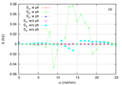
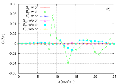
Figure 2: (Color online) Spin polarization $\mathbf{S}=(S_{x},S_{y},S_{z})$ of the central system versus the Rashba coefficient $\alpha$ averaged over the time interval $[180,220]$ ps with (w) (a) $x$-polarized photon field and (b) $y$-polarized photon field or without (w/o) photon cavity ($\beta=0$ and $B=10^{-5}$ T).

Here, we will compare the spin polarization in the central system for $x$- or $y$-polarization of the photon field with the spin polarization in the case that the photon cavity is removed. Figure 2 shows the spin polarization as a function of the Rashba coefficient. The critical value of the Rashba coefficient, which describes the position of the destructive AC interference is $\alpha^{c}\approx 13$ meV nm, where the TL charge current has a pronounced minimum [53]. The spin polarization is largest around $\alpha=\alpha^{c}$ due to spin accumulation in the current suppressed regime. For $\alpha\to 0$, the spin polarization should vanish, except for the minor spin polarization in $S_{z}$ due to the Zeeman interaction with the small magnetic field. Apart from that, only the $S_{y}$ spin polarization seems to be significant in Fig. 2.

The direction of the spin polarization vector can be explained with the concept of the effective magnetic field,

$$\hat{\mathbf{B}}_{R}=-\frac{\hat{\mathbf{p}}\times\mathbf{E}}{m^{*}c},$$ (45)

occurring due to the electronic motion in the electric field $\mathbf{E}=E\mathbf{e}_{z}$. Consequently, we can write the Rashba term

$$\hat{H}_{R}=\frac{\alpha^{\prime}}{\hbar}\mathbf{\bm{\sigma}}\cdot(\hat{\mathbf{p}}\times\mathbf{E})=-\frac{\alpha^{\prime}m^{*}c}{\hbar}\bm{\sigma}\cdot\hat{\mathbf{B}}_{R}$$ (46)

with $\alpha^{\prime}=\alpha/E$. The spin polarization densities vanish in a one-dimensional (1D) ring with only Rashba SOI due to Kramers degeneracy for the time-reversal symmetric system (see also Ref. [53]). It is therefore clear that the spin polarization densities in the case without photon cavity result only from the geometric deviations from the 1D ring model, for example, the contact regions. The main transport and canonical momentum in the contact regions is along the $x$-direction. As a consequence, the Rashba effective magnetic field, $\hat{\mathbf{B}}_{R}$, should be parallel to the $y$-direction and induce a spin polarization in mainly the $y$-direction as is in fact depicted in Fig. 2. With photon cavity, the $x$-polarized photons should lead to an additional kinetic momentum of the electrons in $x$-direction increasing the $S_{y}$ spin polarization further. This is also very well in agreement with Fig. 2(a). However, it is interesting that the $y$-polarized photons do not induce an $S_{x}$ spin polarization although the vector potential contribution to the kinetic momentum would suggest this. Here, the reason for the vanishing $S_{x}$ and $S_{z}$ spin polarization is that the spin polarization density distribution for the $S_{x}$ and $S_{z}$ spin polarization is constrained to an antisymmetric function in $y$ around the x-axis ($y=0$) for any time $t$, when the central system is initially empty ($N_{e,\rm{init}}=0$). The spin polarization density distribution for spin polarization $S_{y}$ is symmetric around $y=0$ permitting the non-vanishing spin-polarization $S_{y}$. As a result, the $y$-polarized photon field increases only the $S_{y}$ spin polarization, but less than in the $x$-polarized case (Fig. 2(b). The symmetry properties and, as a consequence, the non-vanishing components of the spin polarization change if $N_{e,\rm{init}}>0$. Alternatively, $S_{x}\not\approx 0$ and $S_{z}\not\approx 0$ could be achieved with a circularly polarized photon field.

3.2 Circular photon field polarization

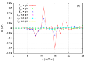
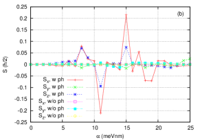
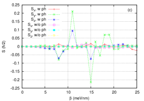
Figure 3: (Color online) Spin polarization $\mathbf{S}=(S_{x},S_{y},S_{z})$ of the central system averaged over the time interval $[180,220]$ ps with (w) or without (w/o) photon cavity and (a) LH circularly polarized photon field versus the Rashba coefficient $\alpha$ ($\beta=0$), (b) RH circularly polarized photon field versus the Rashba coefficient $\alpha$ ($\beta=0$) and (c) RH circularly polarized photon field versus the Dresselhaus coefficient $\beta$ ($\alpha=0$).

The circularly polarized photon field has a non-vanishing spin angular momentum perturbing the angular orbital motion of the electrons. Electrons in a 1D ring geometry (as an approximation of our geometry) do not show a circular charge current for vanishing magnetic field [53], but placing them in a photon cavity with circularly polarized photon field would let them move around the ring due to the spin angular momentum of light. The circular motion is a much stronger perturbation of the ring electrons than the perturbation caused by the linearly polarized photon field. The angular electronic motion in the electric field causes an effective magnetic field and a local spin polarization in radial direction. In our 2D geometry, we will see that the circularly polarized photon field induces also vortices of the size of the ring width. As a consequence, the spin polarization is not only a local quantity. It should be substantially larger than for linear polarization due to the strong perturbation of the circularly polarized photon field with the electronic system.

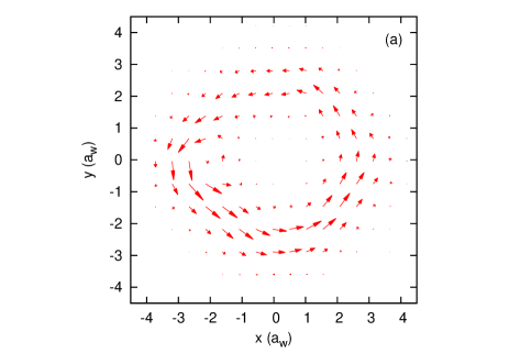
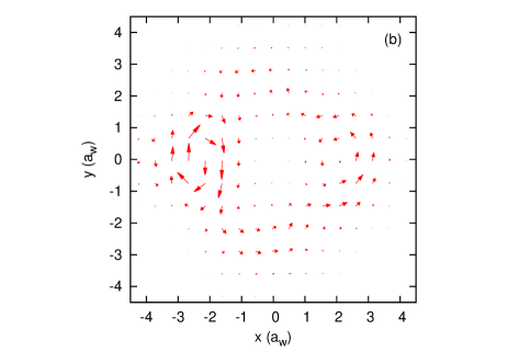
Figure 4: (Color online) Normalized vector fields of the charge current density $\mathbf{j}^{c}(x,y)$ in the central system for (a) the Rashba coefficient $\alpha=11$ meV nm and (b) $\alpha=15$ meV nm at $t=200$ ps with RH circularly polarized photon field and Dresselhaus coefficient $\beta=0$.

Figure 3 shows the spin polarization for (a) LH circularly polarized photon field and (b) and (c) RH circularly polarized photon field. Different from all other subfigures of Fig. 2 and Fig. 3, Fig. 3(c) shows the spin polarization as a function of the Dresselhaus instead of the Rashba coefficient. The spin polarization is indeed substantially larger for circular polarization than for linear polarization, Fig. 2. Furthermore, the spin polarization could take any direction due to spin precession. This is a fundamental difference between the linearly and circularly polarized photon field, where only the $S_{y}$ spin polarization was substantially different from zero. Only the circularly polarized photon field can induce $S_{x}$ spin polarization although the $y$-polarized photon field leads to an effective magnetic field in $x$-direction.

It might seem surprising that the $S_{y}$ spin polarization is relatively small for the circularly polarized photon field. Figure 4 shows the normalized vector field for the charge current density $\mathbf{j}^{c}(x,y)$ for RH circularly polarized photon field and two values of the Rashba coefficient, symmetrically located around $\alpha=\alpha^{c}$. The vortices disappear or are much weaker without photon cavity or with linearly polarized photon field. They are also weaker for circularly polarized photon field and Rashba coefficient values, which are associated with a smaller spin polarization. The charge current density is in general a complicated superposition of many vortices. We would like to mention that it is important that we have used a ring geometry with a finite width. Otherwise, our numerical calculations would not give a realistic picture of the spin polarization. The relatively strong vortices in Fig. 4, which are located close to the contact regions to the leads, are usually not as symmetric in $x$-direction around their center than they are in $y$-direction. Correspondingly, there is often a relatively strong net $y$-component of the canonical momentum leading to a Rashba effective magnetic field in $x$-direction and a much stronger $S_{x}$ spin polarization than $S_{y}$ spin polarization.

It is in particular interesting to observe the local antisymmetric behavior of the $x$- and $z$-component of the spin polarization around the level crossings at $\alpha=\alpha^{c}$ (Fig. 3(b)), which are the spin polarizations induced by the circularly polarized photon field. By contrast, the $S_{y}$ spin polarization is clearly not antisymmetric around $\alpha=\alpha^{c}$ for the linearly polarized photon field (see Fig. 2). It can be seen from a comparison of Fig. 4(a), where $\alpha<\alpha^{c}$, and Fig. 4(b), where $\alpha>\alpha^{c}$, that the circulation direction of the strong vortex at the left contact region is inversed. This leads to the local antisymmetric behavior of the $S_{x}$ and $S_{z}$ spin polarization around $\alpha=\alpha^{c}$. Since the pronounced vortex structure is mainly due to the circular polarization of the photon field, only the components of the spin polarization, which are induced by the circularly polarized cavity photon field show the local antisymmetric behavior. The fact that the $S_{y}$ spin polarization is not antisymmetric for linear photon field polarization can be understood as follows: qualitatively, as said before, only the canonical momentum due to the deviations from the 1D ring geometry (and the photon cavity, which is unimportant for $S_{y}$ in the case of circular photon field polarization) allows for spin polarization in the central system. The contact regions in $x$-direction cause only smaller perturbations of the central system spectrum beyond the level-crossing structure from the 1D ring geometry (which only the circularly polarized photon field can perturb). It is not likely that these smaller perturbations would lead to additional level-crossings around $\alpha\approx 13$ meV nm, which we have found to be responsible for the antisymmetric behavior of $S_{x}$ and $S_{z}$ for circular polarization. Therefore, a local antisymmetry of $S_{y}$ around $\alpha\approx 13$ meV nm cannot be found.

The $x$- and $z$-components of the spin polarization are also antisymmetric with respect to the handedness of the circularly polarized light (Fig. 3(a) in comparison with Fig. 3(b)). As the $S_{x}$ and $S_{z}$ spin polarization are a direct and pure consequence of circular polarization meaning that they are vanishing in the case without photon cavity and in the case with linear polarized photon field, it is understandable that a sign change in the handedness would follow a sign change in the effective magnetic field and spin polarization. In fact, also the vortex circulation direction is inversed by an inversion of the handedness of the circularly polarized photon field. The situation is different for the $S_{y}$ spin polarization, which is different from zero in the absence of photons. The circularly polarized photon field changes the $S_{y}$ spin polarization only slightly. Furthermore, comparing the Rashba and Dresselhaus case for RH circularly polarized photon field (Fig. 3(b) and Fig. 3(c)), we can verify the spin polarization symmetries

$$\left(\begin{array}[]{c}S_{xD}\\ S_{yD}\\ S_{zD}\end{array}\right)=-\left(\begin{array}[]{c}S_{yR}\\ S_{xR}\\ S_{zR}\end{array}\right)$$ (47)

due to the structure of the Rashba and Dresselhaus Hamiltonian.

4 Charge and spin polarization currents

Here, we show our numerical results for the charge and spin polarization currents, both between the leads and the system and in the system (quantum ring) itself. Emphasis is laid on the phenomena caused by the photon cavity with a focus on the circularly polarized photon field.

4.1 Non-local currents

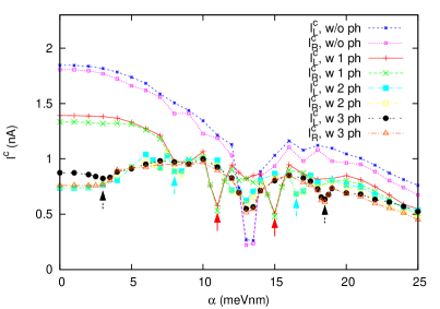
Figure 5: (Color online) Non-local lead-system charge currents $I^{c}_{L}$ and $I^{c}_{R}$ versus the Rashba coefficient $\alpha$ at time $t=200$ ps and with RH circularly polarized photon field for different initial number of photons $N_{ph,\rm init}=0,1,2,3$. The Dresselhaus coefficient $\beta=0$.

Figure 5 shows the non-local (lead-ring) charge currents from the left lead into the system and further into the right lead as a function of the Rashba coefficient $\alpha$ at time $t=200$ ps and circularly polarized photon field. We note in passing that the result depends not on the handedness of the circularly polarized light. Left- or right-handedness would only interchange the meaning of the otherwise indifferent upper and lower ring arm. With increasing initial number of photons the current tends to get suppressed due to the in general smaller energy differences between the MB levels and the fact that the states having a larger photon content lie in general higher in energy. However, more interestingly, we observe two additional current dips for smaller and larger $\alpha$, while the current dip at $\alpha=\alpha^{c}$ appears weaker. With increasing number of initial photons, the two dips for smaller or larger Rashba coefficient move to even smaller ($\alpha\approx\{11,8,3\}$ meV nm) or larger ($\alpha\approx\{15,16.5,18.5\}$ meV nm) Rashba coefficients, respectively, as the initial photon number increases ($N_{ph,\rm init}=\{1,2,3\}$). The dips are indicated in Fig. 5 by arrows in the color of the charge current from the left lead, $I^{c}_{L}$. The circularly polarized photon field has a spin angular momentum, which is proportional to the number of photons in the system. The spin angular momentum of the photons interacts with the total (orbital and spin) angular momentum of the electrons in the ring. For a one-dimensional ring of radius $a$ with only Rashba interaction [53] the electron states are fourfold degenerate at $\alpha=0$ and in general twofold degenerate for $\alpha>0$, as will be explained here in detail. The eigenstates are

$$\Psi_{\nu n}^{R}(\varphi) = \left(\begin{array}[]{c}\Psi_{\nu n}^{R}(\varphi,\uparrow)\\ \Psi_{\nu n}^{R}(\varphi,\downarrow)\end{array}\right)$$ (50)

$$= \frac{\exp(in\varphi)}{\sqrt{2\pi a}}\left(\begin{array}[]{c}A_{\nu,1}^{R}\\ A_{\nu,2}^{R}\exp(i\varphi)\end{array}\right)$$ (53)

with the $2\times 2$ coefficient matrix

$$A^{R}=\left(\begin{array}[]{cc}A_{\nu,1}^{R}&A_{\nu,2}^{R}\end{array}\right)=\left(\begin{array}[]{cc}\cos\left(\frac{\theta_{R}}{2}\right)&\sin\left(\frac{\theta_{R}}{2}\right)\\ \sin\left(\frac{\theta_{R}}{2}\right)&-\cos\left(\frac{\theta_{R}}{2}\right)\end{array}\right),$$ (54)

$$\tan\left(\frac{\theta_{R}}{2}\right)=\frac{1-\sqrt{1+x_{R}^{2}}}{x_{R}}$$ (55)

and the dimensionless Rashba parameter, $x_{R}$ (and Dresselhaus parameter, $x_{D}$) is defined by

$$\left(\begin{array}[]{c}x_{R}\\ x_{D}\end{array}\right):=\frac{2m^{*}a}{\hbar^{2}}\left(\begin{array}[]{c}\alpha\\ \beta\end{array}\right).$$ (56)

We remind the reader that $a$ is the ring radius. We call $n$ the total angular momentum quantum number and $\nu=\pm 1$ the spin quantum number (the latter according to the cardinality of the set of possible values). One can show that $n$ describes indeed the total (i.e. spin and orbital) angular momentum:

$$\bra{\nu n}\hat{J}_{z}\ket{\nu n} = \bra{\nu n}\hat{L}_{z}+S_{z}\ket{\nu n}$$ (57)

$$= \bra{\nu n}\frac{\hbar}{i}\frac{\partial}{\partial\varphi}+\frac{\hbar}{2}\sigma_{z}\ket{\nu n}$$

$$= \hbar\left(n+\frac{1}{2}\right).$$

In the Dresselhaus case, $\bra{\nu n}\hat{J}_{z}\ket{\nu n}$ in Eq. (57) would depend on $n$ and $x_{D}$ since $[\hat{J}_{z},\hat{H}_{D}]\neq 0$. We note in passing that $[\hat{J}_{z},\hat{H}_{R}]=0$ such that, in the Rashba case, $J_{z}=n+1/2$ is indeed a “good” quantum number (constant). Furthermore, one can define a quantum number

$$m:=\nu\left(n+\frac{1}{2}\right)+\frac{1}{2}=\nu\frac{\bra{\nu n}\hat{J}_{z}\ket{\nu n}}{\hbar}+\frac{1}{2}.$$ (58)

While the exact physical meaning of $m$ and $\nu$ remains unclear, these quantum numbers are convenient to describe the degeneracies in the 1D Rashba ring. (We assume that they both contain angular momentum and therefore reflect the spin angular momentum of light.) States with the same $m$, but different $\nu$ are degenerate for all $\alpha$. Additional degeneracies in $m$ appear at $\alpha=0$ and further single points, where the states are four fold degenerate in total.

How can the degeneracy in $\nu$ be lifted? As said before, most likely, the spin quantum number $\nu$ contains inherently also orbital angular momentum. It is though clear, that is contains angular momentum of some kind. As a consequence, we expect that the circularly polarized photon field would have a different influence on states of different $\nu$ (because of the different angular momentum content), which would imply that it could lift the degeneracy. However, we would not expect that the linearly polarized photon field could lift the degeneracy, as it couples not to the angular momentum. Only the circularly polarized photon field with a non-vanishing spin angular momentum can therefore lift the degeneracy in $\nu$. It is interesting to note that for the two-dimensional ring without photons (Fig. 6(a)) or linearly polarized photons (Fig. 6(b)), the states are in general double degenerate for all values of $\alpha$ except single crossing points. The $m$-degeneracy at $\alpha=0$ is split due to the 2D geometry. The $\nu$-degeneracy and its energy splitting for $\alpha>0$ by the circularly polarized photon field is here of main interest (Fig. 6). We would like to draw the attention of the reader to subtle difference between the 1D and 2D case. First, we consider the 1D case with two states with different $m$, which are splitted in energy for $\alpha>0$. Second, we consider the 2D case with circularly polarized photon field with two states with different $\nu$, which are splitted in energy for $\alpha>0$. In both cases, we look at the crossings at $\alpha>0$ around the critical values in $\alpha$ corresponding to the AC phase differences $\Delta\Phi=n\pi$ with $n=1,2,\dots$. Then, the difference can be stated as follows: in the 1D case one state crosses with a state that is lower, and the other state, with a state that is higher in energy at $\alpha=0$; in the 2D case the two states cross also with two other states, but here the latter are degenerate at $\alpha=0$.

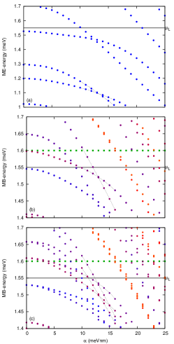
Figure 6: (Color online) Many-electron (ME) or many-body (MB) energy spectrum of the system Hamiltonian Eq. (2) versus the Rashba coefficient $\alpha$ (a) without photon cavity, (b) with $x$-polarized photon field and (c) with RH circularly polarized photon field. The states are differentiated according to their electron content $N_{e}$ by the shape of the dots and according to their fractional photon content $N_{ph}$ by their color. Zero-electron states ($N_{e}=0$, 0ES) are represented as filled squares (the green color means that $N_{ph}=4$) and single electron states ($N_{e}=1$, SES) as filled circles with the continuous color spectrum from blue over red to yellow corresponding to the range $N_{ph}\in[0,3]$. The chemical potential $\mu_{L}$ of the left lead is shown by a solid black line. The mostly occupied states, which contribute to the current dips, are connected by black dotted lines close to their crossings as a guide to the eye. Note that the spectra are shown for different energy ranges.

To understand the three dips in the non-local (lead-ring) charge current better, we take a look at the MB spectrum. Figure 6 shows the energy spectrum of the central system versus the Rashba coefficient. We note that Fig. 6(c) is independent of the handedness of the circularly polarized photon field. The state crossing of the mostly occupied states leading to dips in the non-local charge current are shown by dotted black lines. These states include at least about 50% of the charge in the central quantum ring system. The zero-electron states are shown by filled squares and the SES by filled circles. The photon content, which can be a fractional number due to the light-matter coupling is shown by a continuous range of colors. A photon content of $N_{ph}=0$ is shown in blue, $N_{ph}=1.5$ is shown in red and $N_{ph}=3$ is shown in yellow. $N_{ph}=4$ is shown in green color. When we start with one photon initially, $N_{ph,\rm init}=1$, the MB spectrum for the linearly and circularly polarized fields shown in Fig. 6(b) and (c) lead to the situation that the mostly occupied states are states with a photon content $N_{ph}\approx 1$. These states have a color close to purple or violet red and lie $0.4$ meV higher in the spectrum than the mostly occupied states without photon cavity (which have of course photon content $N_{ph}=0$), see Fig. 6(a).

In the case without photons, Fig. 6(a), and with linearly polarized photon field, Fig. 6(b), the SES are double degenerate, but become split for $\alpha>0$ in the case of circularly polarized photon field, Fig. 6(c). Consequently, without photon cavity or for linearly polarized photons, the four crossings of the four mostly occupied states are at one value of $\alpha=\alpha^{c}$. With circularly polarized photon field, the four crossings of the four mostly occupied states become to lie at three different values of $\alpha$. Two crossings are at the intermediate $\alpha$-value, which is located close to $\alpha^{c}$, the third crossing is at $\alpha<\alpha^{c}$ and the fourth is at $\alpha>\alpha^{c}$. The three MB crossing locations in the circularly polarized photon field case are the reason for the three dips of the non-local (lead-ring) charge current. To summarize the essence of Fig. 6, each Rashba coefficient $\alpha$ with a crossing of the mostly occupied states is corresponding to a dip of the non-local charge current. Without photon cavity or for linearly polarization of the photon field, we have one Rashba coefficient, $\alpha^{c}$, with crossings and therefore one dip — for circular polarization, we have three values of the Rashba coefficient with crossings and therefore three dips.

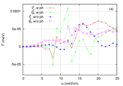
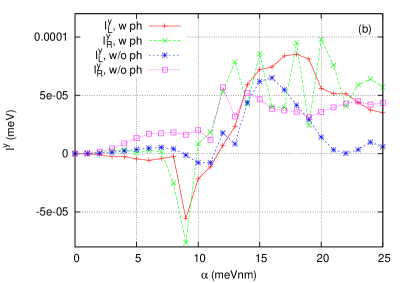
Figure 7: (Color online) Non-local spin polarization currents $I_{L}^{y}$ and $I_{R}^{y}$ into and out of the central system versus the Rashba coefficient $\alpha$ averaged over the time interval $[180,220]$ ps with (w) (a) $x$-polarized photon field and (b) $y$-polarized photon field or without (w/o) photon cavity. $I_{L}^{x}$, $I_{L}^{z}$, $I_{R}^{x}$ and $I_{R}^{z}$ are not shown as they are vanishing. The Dresselhaus coefficient $\beta=0$.

Figure 7 shows the non-local (lead-ring) spin polarization currents for (a) $x$-polarized photon field and (b) $y$-polarized photon field from the left lead into the system $\mathbf{I}_{L}=(I_{L}^{x},I_{L}^{y},I_{L}^{z})$ or from the system to the right lead $\mathbf{I}_{R}=(I_{R}^{x},I_{R}^{y},I_{R}^{z})$. Similarly to the spin polarization, Fig. 2, the $y$-polarized photons do not induce a non-local current for $S_{x}$ spin polarization neither from the left nor to the right lead. Also the non-local current for $S_{z}$ spin polarization is vanishing. In the strong Rashba regime $\alpha\in[19,24]$ meV nm, the $S_{y}$ spin polarization is overall emptied in the system without photon cavity meaning that $I_{L}^{y}<I_{R}^{y}$, however, with $x$-polarized photon field, we observe in total $S_{y}$ spin injection ($I_{L}^{y}>I_{R}^{y}$). The $y$-polarized photon field is not in general able to invert the spin emptying into spin injection in the strong Rashba regime given above.

4.2 Local photocurrents

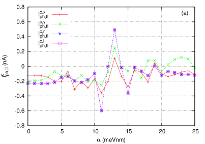
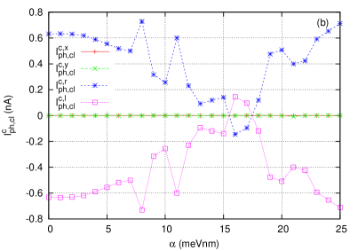
Figure 8: (Color online) (a) TL and (b) CL charge photocurrents $I^{c,p}_{\rm ph,tl}$ versus the Rashba coefficient $\alpha$ averaged over the time interval $[180,220]$ ps with ($p=x$) $x$-polarized photon field, ($p=y$) $y$-polarized photon field, ($p=r$) RH circularly polarized photon field and ($p=l$) LH circularly polarized photon field. The Dresselhaus coefficient $\beta=0$.

Figure 8 shows the TL and CL charge photocurrents. The photon cavity reduces in general the TL charge current (Fig. 8(a)) (negative photocurrent). However, at the destructive AC interference at $\alpha=\alpha^{c}$, the TL charge current is enhanced in particular for the circularly polarized photon field. By the photonic perturbation of the AC phase difference, the electrons can flow more freely through the ring and the electron dwell time is reduced. In the case of the circularly polarized photon field, at the smaller and larger values $\alpha\approx\{11,15\}$ meV nm, where the additional non-local (lead-ring) charge current dips appear (Fig. 5), the TL charge photocurrent is very negative. This gives some further evidence about the photonic nature of the additional non-local charge current dips. The TL current is independent of the handedness of the circularly polarized photon field since the ring is otherwise symmetric with respect to the $x$-axis. The CL charge photocurrent has different sign for RH or LH circularly polarized photon field since the circular motion of electrons changes with the spin angular momentum of the photons in sign (Fig. 8(b)). In contrast, the CL charge current remains uninfluenced by the linearly polarized photon field. With the aid of the angular motion of electrons induced by the circularly polarized photon field, the charge flow can be controlled to pass through the upper or lower ring arm. Around the destructive AC interference, the CL charge photon current gets suppressed due to the unfavorable phase relation. The suppression spans a relatively wide region $\alpha\in[9,23]$ meV nm when compared to the non-local charge current dip. The CL charge photon current might therefore serve as an alternative tool to detect AC phase interference phenomena, which minimizes the likelihood to overlook an AC destructive phase interference because of the narrowness of the non-local charge current dip in the parameter space (consider for example the dip at $\alpha=\alpha^{c}$ in Fig. 5). We note that the TL and CL charge current is independent from the kind of SOI, i.e. Rashba or Dresselhaus, as it is a spin-independent quantity.

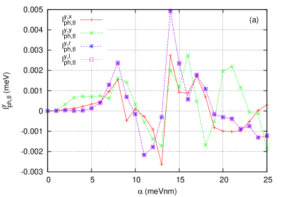
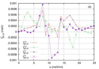
Figure 9: (Color online) (a) TL spin photocurrents for spin polarization $S_{y}$, $I^{y}_{\rm ph,tl}$ and (b) CL spin photocurrents for spin polarization $S_{z}$, $I^{z}_{\rm ph,cl}$, versus the Rashba coefficient $\alpha$ averaged over the time interval $[180,220]$ ps with ($p=x$) $x$-polarized photon field, ($p=y$) $y$-polarized photon field, ($p=r$) RH circularly polarized photon field and ($p=l$) LH circularly polarized photon field. The Dresselhaus coefficient $\beta=0$.

Figure 9 shows the TL spin photocurrent for the spin polarization $S_{y}$ and the CL spin photocurrent for the spin polarization $S_{z}$. As opposed to the charge photocurrents, the spin photocurrents drop to zero for the Rashba coefficient $\alpha\to 0$ (when only a very weak Zeeman term distinguishes the spin). The influence of the circularly polarized photon field is strong in a relatively wide range around the position of the destructive AC phase at $\alpha=\alpha^{c}$ and weak around the constructive AC phases ($\alpha=0$ meV nm and $\alpha\approx 21$ meV nm). For the destructive AC phase, the reduced electron mobility increases the electron dwell time leading to the strong spin photocurrents. In general, the influence of the circularly polarized photon field is a bit stronger than the influence of the linearly polarized photon field. We note in passing that the other spin photocurrents, which are not shown, $I^{x}_{\rm ph,tl}$, $I^{x}_{\rm ph,cl}$, $I^{y}_{\rm ph,cl}$ and $I^{z}_{\rm ph,tl}$, are about one order of magnitude smaller than $I^{y}_{\rm ph,tl}$ and $I^{z}_{\rm ph,cl}$. The local spin polarization currents without photons, $I^{y,0}_{tl}$ and $I^{z,0}_{cl}$, were also much larger than $I^{x,0}_{tl}$, $I^{x,0}_{cl}$, $I^{y,0}_{cl}$ and $I^{z,0}_{tl}$, meaning that the photon cavity is not changing the set of major local spin polarization currents. It is interesting to note that the handedness of the circularly polarized photon field does not affect the major spin photocurrents including even the CL spin photocurrent $I^{z}_{\rm ph,cl}$.

5 Conclusions

The interaction between spin-orbit coupled electrons in a quantum ring interferometer and a circularly polarized electromagnetic field shows a variety of interesting effects, which do not appear for linear polarization of the photon field. The AC phase that controls the transport of electrons in such a quantum device is influenced by the photons. We found that the spin polarization in a ring, which is connected to leads and mirror symmetric with respect to the transport axis, is perpendicular to the transport direction. A linearly polarized photon field with polarization in or perpendicular to the transport direction, increases only the magnitude of the spin polarization while keeping the direction of the spin polarization vector uninfluenced. The spin polarization accumulates to larger magnitudes when the transport of electrons is suppressed by a destructive AC phase. The circularly polarized photon field enhances the spin polarization much more than the linearly polarized photon field. Furthermore, the spin polarization vector is no longer bound to a specific direction as the circularly polarized photon field excites the orbital angular motion of the electrons around the ring and pronounced vortices of the charge current density of smaller spatial scale. The latter show the importance to resolve the finite width of our ring as we did in our model. The circulation direction of the vortices is found to depend on the handedness of the photon field and the value of the Rashba coefficient $\alpha$ relative to $\alpha^{c}$.

The charge current from the left lead into the quantum ring device and out to the right lead shows three AC dips around $\alpha^{c}$ instead of one for the circularly polarized photon field. The reason for it is a small splitting of degenerate states by the interaction of the angular momentum of the electrons and the spin angular momentum of light, which leads to MB crossings at three different values of the Rashba coefficient. The distance in $\alpha$ between the dips increases with the number of photons in the system due to the larger spin angular momentum of light. The charge photocurrent from the left to the right side of the quantum ring is usually negative meaning that the photon cavity suppresses the charge transport thus increasing the device resistance (except close to $\alpha^{c}$, where the AC phase interference is destructive). The circulating part of the charge photocurrent can only be excited by the circularly polarized photon field. The handedness of the circulation depends on the handedness of the light. This way, it is possible to confine the charge transport through the ring to one ring arm (upper or lower). The circular charge photocurrent is suppressed in a wide range of the Rashba coefficient around $\alpha=\alpha^{c}$ and might therefore serve as a reliable quantity to detect destructive AC phases. The spin photocurrents are especially strong around $\alpha=\alpha^{c}$ (due to the longer electron dwell time) and for circular polarization (for geometrical reasons). The handedness of the light does not influence the spin polarization current including the current for $S_{z}$ spin polarization, which circulates around the ring.

In summary, strong spin polarization, spin photocurrents and charge current vortices as well as splitting of the AC charge current dip into three dips and control over the local charge flow through the ring arms are important effects that only appear for circularly polarized photon field. These effects are crucial to know about for the development of spin-optoelectronic quantum devices in the field of quantum information processing. For instance, interest might arise to build a spintronic device, which breaks (blocks) an electrical circuit if the gate voltage is not precisely equal to a specific, sharply defined critical value, which corresponds to the magnitude of the electric field leading to a destructive AC phase interference in a ring interferometer. The critical gate potential of the quantum switch could be adjusted by variation of the ring radius [53]. A possible experimental approach to determine the ring radius would be to measure the circular charge current around the ring (for example indirectly by its induced magnetic field) that is caused by a circularly polarized cavity photon field. We predict that this approach is better than direct resistance measurements of the quantum switch without the photon cavity. This is because the data that a certain number of measurements with the circularly polarized cavity photon field yields are more relevant for suggesting the proper ring radius due to the broadness of the corresponding Aharonov-Casher feature in the Rashba coefficient.

Appendix A Parameters used for the numerical results

We assume GaAs-based material with electron effective mass $m^{*}=0.067m_{e}$ and background relative dielectric constant $\kappa=12.4$. As stated earlier, the Rashba coefficient $\alpha$ can be tuned by changing the magnitude of an electric field, which is perpendicular to the plane containing the quantum ring structure. The range of $\alpha$ investigated in this paper is about one order of magnitude larger than typical values of $\alpha$ for GaAs. However, we point out that the predicted features are at fixed positions in $x_{R}$ (Eq. (56)) and not in $\alpha$. Therefore, by increasing the ring radius, experiments could be performed in a smaller range of the Rashba coefficient if it seems difficult to increase the electric field sufficiently by a gate. For our numerical calculations, it is inconvenient to increase the ring radius further, as we would have to consider a larger number of many-body states to get converged results. With the state of the art computational facilities, however, we are limited to about $200$ many-body states for our numerically exact approach. Alternatively, other materials as InAs could be used, for which the the Rashba coefficient is about one order of magnitude larger [60]. The Dresselhaus coefficient $\beta$ is determined by the bulk properties of the material and could only be changed by using a different material. The value for GaAs would be $\beta=3.0$ meV nm. When using $\beta>0$, we would also decrease slightly the $\alpha$-range for which our features due to the destructive AC phase appear. However, our features would become more complex when both Rashba and Dresselhaus spin-orbit interaction are present [23].

We consider a single photon cavity mode with fixed photon excitation energy $\hbar\omega=0.4$ meV. The electron-photon coupling constant in the central system $g^{EM}=0.1$ meV. The temperature of the reservoirs is $T=0.5$ K. The chemical potentials in the leads are $\mu_{L}=1.55$ meV and $\mu_{R}=0.7$ meV leading to a source-drain electrical bias window $\Delta\mu=0.85$ meV.

A very small external uniform magnetic field $B=10^{-5}$ T is applied through the central ring system and the lead reservoirs to lift the spin degeneracy in the numerical calculations. The applied magnetic field $B<<B_{0}=\Phi_{0}/A\approx 0.2$ T is order of magnitudes outside the AB regime. The two-dimensional magnetic length would be very large: $l=[c\hbar/(eB)]^{1/2}=8.12$ $\mu$m. However, the parabolic confinement of the ring system in $y$-direction leads to the much shorter magnetic length scale

$$a_{w} =\left(\frac{\hbar}{m^{*}\Omega_{0}}\right)^{1/2}\frac{1}{\sqrt[4]{1+[eB/(m^{*}c\Omega_{0})]^{2}}}$$ (59)

$$\approx\left(\frac{\hbar}{m^{*}\Omega_{0}}\right)^{1/2}=33.7\ {\rm nm}.$$

To model the coupling between the system and the leads, we let the affinity constant $\Delta_{E}^{l}=0.25$ meV to be close to the characteristic electronic excitation energy in $x$-direction. In addition, we let the contact region parameters for lead $l\in\{L,R\}$ in $x$- and $y$-direction be $\delta^{l}_{x}=\delta^{l}_{y}=4.39\times 10^{-4}$ $\rm{nm}^{-2}$. The system-lead coupling strength $g_{0}^{l}=1.371\times 10^{-3}$ ${\rm meV}/{\rm nm}^{3/2}$. Before switching on the system-lead coupling at $t=0$ with the time-scale $(\alpha^{l})^{-1}=3.291$ ps, we assume the central system to be in the pure state with electron occupation number $N_{e,\rm{init}}=0$ and — unless otherwise stated — photon occupation number $N_{ph,\rm{init}}=1$. The SES charging time-scale $\tau_{\rm SES}\approx 30$ ps, and the two-electron state (2ES) charging time-scale $\tau_{\rm 2ES}\gg 200$ ps, which is described in the sequential tunneling regime. We study the non-equilibrium transport properties around $t=200$ ps, when the system has not yet reached a steady state. Some dynamical observables are averaged over the time interval $[180,220]$ ps to give a more representative picture in the transient regime. The charge in the quantum ring system at $t=200$ ps is typically of the order of $Q(t=200\rm{ps})\approx 1e$.

Appendix B Operators for the charge and spin polarization density and charge and spin polarization current density

The charge density operator

$$\hat{n}^{c}(\mathbf{r})=e\hat{\mathbf{\Psi}}^{\dagger}(\mathbf{r})\hat{\mathbf{\Psi}}(\mathbf{r})$$ (60)

and the spin polarization density operator for spin polarization $S_{i}$

$$\hat{n}^{i}(\mathbf{r})=\frac{\hbar}{2}\hat{\mathbf{\Psi}}^{\dagger}(\mathbf{r})\sigma_{i}\hat{\mathbf{\Psi}}(\mathbf{r}).$$ (61)

The component labeled with $j\in\{x,y\}$ of the charge current density operator

$$\hat{j}^{c}_{j}(\mathbf{r}) = \frac{e\hbar}{2m^{*}i}\left[\hat{\mathbf{\Psi}}^{\dagger}(\mathbf{r})\nabla_{j}\hat{\mathbf{\Psi}}(\mathbf{r})-\left(\nabla_{j}\hat{\mathbf{\Psi}}^{\dagger}(\mathbf{r})\right)\hat{\mathbf{\Psi}}(\mathbf{r})\right]$$ (62)

$$+\frac{e^{2}}{m^{*}c}\hat{A}_{j}(\mathbf{r})\hat{\mathbf{\Psi}}^{\dagger}(\mathbf{r})\hat{\mathbf{\Psi}}(\mathbf{r})$$

$$+\frac{e}{\hbar}\hat{\mathbf{\Psi}}^{\dagger}(\mathbf{r})(\beta\sigma_{x}-\alpha\sigma_{y})\hat{\mathbf{\Psi}}(\mathbf{r})\delta_{x,j}$$

$$+\frac{e}{\hbar}\hat{\mathbf{\Psi}}^{\dagger}(\mathbf{r})(\alpha\sigma_{x}-\beta\sigma_{y})\hat{\mathbf{\Psi}}(\mathbf{r})\delta_{y,j}$$

with the space-dependent vector potential including the static magnetic field and cavity photon field part

$$\hat{\mathbf{A}}(\mathbf{r})=\mathbf{A}(\mathbf{r})+\hat{\mathbf{A}}^{\mathrm{ph}}(\mathbf{r}).$$ (63)

The current density operator for the $j$-component and $S_{x}$ spin polarization

$$\hat{j}^{x}_{j}(\mathbf{r}) = \frac{\hbar^{2}}{4m^{*}i}\left[\hat{\mathbf{\Psi}}^{\dagger}(\mathbf{r})\sigma_{x}\nabla_{j}\hat{\mathbf{\Psi}}(\mathbf{r})\right.$$ (64)

$$-\left.\left(\nabla_{j}\hat{\mathbf{\Psi}}^{\dagger}(\mathbf{r})\right)\sigma_{x}\hat{\mathbf{\Psi}}(\mathbf{r})\right]$$

$$+\frac{e\hbar}{2m^{*}c}\hat{A}_{j}(\mathbf{r})\hat{\mathbf{\Psi}}^{\dagger}(\mathbf{r})\sigma_{x}\hat{\mathbf{\Psi}}(\mathbf{r})$$

$$+\frac{\beta\delta_{x,j}+\alpha\delta_{y,j}}{2}\hat{\mathbf{\Psi}}^{\dagger}(\mathbf{r})\hat{\mathbf{\Psi}}(\mathbf{r}).$$

the current density operator for $S_{y}$ spin polarization

$$\hat{j}^{y}_{j}(\mathbf{r}) = \frac{\hbar^{2}}{4m^{*}i}\left[\hat{\mathbf{\Psi}}^{\dagger}(\mathbf{r})\sigma_{y}\nabla_{j}\hat{\mathbf{\Psi}}(\mathbf{r})\right.$$ (65)

$$-\left.\left(\nabla_{j}\hat{\mathbf{\Psi}}^{\dagger}(\mathbf{r})\right)\sigma_{y}\hat{\mathbf{\Psi}}(\mathbf{r})\right]$$

$$+\frac{e\hbar}{2m^{*}c}\hat{A}_{j}(\mathbf{r})\hat{\mathbf{\Psi}}^{\dagger}(\mathbf{r})\sigma_{y}\hat{\mathbf{\Psi}}(\mathbf{r})$$

$$-\frac{\alpha\delta_{x,j}+\beta\delta_{y,j}}{2}\hat{\mathbf{\Psi}}^{\dagger}(\mathbf{r})\hat{\mathbf{\Psi}}(\mathbf{r}).$$

and $S_{z}$ spin polarization

$$\hat{j}^{z}_{j}(\mathbf{r}) = \frac{\hbar^{2}}{4m^{*}i}\left[\hat{\mathbf{\Psi}}^{\dagger}(\mathbf{r})\sigma_{z}\nabla_{j}\hat{\mathbf{\Psi}}(\mathbf{r})\right.$$ (66)

$$-\left.\left(\nabla_{j}\hat{\mathbf{\Psi}}^{\dagger}(\mathbf{r})\right)\sigma_{z}\hat{\mathbf{\Psi}}(\mathbf{r})\right]$$

$$+\frac{e\hbar}{2m^{*}c}\hat{A}_{j}(\mathbf{r})\hat{\mathbf{\Psi}}^{\dagger}(\mathbf{r})\sigma_{z}\hat{\mathbf{\Psi}}(\mathbf{r}).$$

References

References

- Aharonov and Bohm [1959] Y. Aharonov, D. Bohm, Phys. Rev. 115 (1959) 485–491. URL: http://link.aps.org/doi/10.1103/PhysRev.115.485. doi:10.1103/PhysRev.115.485.
- Aharonov and Casher [1984] Y. Aharonov, A. Casher, Phys. Rev. Lett. 53 (1984) 319–321. URL: http://link.aps.org/doi/10.1103/PhysRevLett.53.319. doi:10.1103/PhysRevLett.53.319.
- Aharonov and Anandan [1987] Y. Aharonov, J. Anandan, Phys. Rev. Lett. 58 (1987) 1593–1596. URL: http://link.aps.org/doi/10.1103/PhysRevLett.58.1593. doi:10.1103/PhysRevLett.58.1593.
- Berry [1984] M. V. Berry, Proc. R. Soc. Lond. A 392 (1984) 45–57.
- Moskalenko and Berakdar [2008] A. S. Moskalenko, J. Berakdar, Phys. Rev. A 78 (2008) 051804. URL: http://link.aps.org/doi/10.1103/PhysRevA.78.051804. doi:10.1103/PhysRevA.78.051804.
- Xie et al. [2008] Y. Xie, W. Chu, S. Duan, Applied Physics Letters 93 (2008) 023104. URL: http://search.ebscohost.com/login.aspx?direct=true&db=aph&AN=33361228&site=ehost-live.
- Ganichev et al. [2001] S. D. Ganichev, E. L. Ivchenko, S. N. Danilov, J. Eroms, W. Wegscheider, D. Weiss, W. Prettl, Phys. Rev. Lett. 86 (2001) 4358–4361. URL: http://link.aps.org/doi/10.1103/PhysRevLett.86.4358. doi:10.1103/PhysRevLett.86.4358.
- Quinteiro and Berakdar [2009] G. F. Quinteiro, J. Berakdar, Opt. Express 17 (2009) 20465–20475. URL: http://www.opticsexpress.org/abstract.cfm?URI=oe-17-22-20465. doi:10.1364/OE.17.020465.
- Pershin and Piermarocchi [2005] Y. V. Pershin, C. Piermarocchi, Phys. Rev. B 72 (2005) 245331. URL: http://link.aps.org/doi/10.1103/PhysRevB.72.245331. doi:10.1103/PhysRevB.72.245331.
- Kibis [2011] O. V. Kibis, Phys. Rev. Lett. 107 (2011) 106802. URL: http://link.aps.org/doi/10.1103/PhysRevLett.107.106802. doi:10.1103/PhysRevLett.107.106802.
- Kibis et al. [2013] O. V. Kibis, O. Kyriienko, I. A. Shelykh, Phys. Rev. B 87 (2013) 245437. URL: http://link.aps.org/doi/10.1103/PhysRevB.87.245437. doi:10.1103/PhysRevB.87.245437.
- Räsänen et al. [2007] E. Räsänen, A. Castro, J. Werschnik, A. Rubio, E. K. U. Gross, Phys. Rev. Letters 98 (2007) 157404.
- Szafran and Peeters [2005] B. Szafran, F. M. Peeters, Phys. Rev. B 72 (2005) 165301. URL: http://link.aps.org/abstract/PRB/v72/e165301. doi:10.1103/PhysRevB.72.165301.
- Pichugin and Sadreev [1997] K. N. Pichugin, A. F. Sadreev, Phys Rev. B 56 (1997) 9662.
- Webb et al. [1985] R. A. Webb, S. Washburn, C. P. Umbach, R. B. Laibowitz, Phys. Rev. Lett. 54 (1985) 2696–2699. URL: http://link.aps.org/doi/10.1103/PhysRevLett.54.2696. doi:10.1103/PhysRevLett.54.2696.
- Nitta and Bergsten [2007] J. Nitta, T. Bergsten, New Journal of Physics 9 (2007) 341. URL: http://stacks.iop.org/1367-2630/9/i=9/a=341.
- Bychkov and Rashba [1984] Y. A. Bychkov, E. I. Rashba, Journal of Physics C: Solid State Physics 17 (1984) 6039. URL: http://stacks.iop.org/0022-3719/17/i=33/a=015.
- Dresselhaus [1955] G. Dresselhaus, Phys. Rev. 100 (1955) 580–586. URL: http://link.aps.org/doi/10.1103/PhysRev.100.580. doi:10.1103/PhysRev.100.580.
- Frustaglia and Richter [2004] D. Frustaglia, K. Richter, Phys. Rev. B 69 (2004) 235310. URL: http://link.aps.org/doi/10.1103/PhysRevB.69.235310. doi:10.1103/PhysRevB.69.235310.
- Ying-Fang et al. [2004] G. Ying-Fang, Z. Yong-Ping, L. Jiu-Qing, Chinese Physics Letters 21 (2004) 2093. URL: http://stacks.iop.org/0256-307X/21/i=11/a=006.
- Aronov and Lyanda-Geller [1993] A. G. Aronov, Y. B. Lyanda-Geller, Phys. Rev. Lett. 70 (1993) 343–346. URL: http://link.aps.org/doi/10.1103/PhysRevLett.70.343. doi:10.1103/PhysRevLett.70.343.
- Yi et al. [1997] Y.-S. Yi, T.-Z. Qian, Z.-B. Su, Phys. Rev. B 55 (1997) 10631–10637. URL: http://link.aps.org/doi/10.1103/PhysRevB.55.10631. doi:10.1103/PhysRevB.55.10631.
- Wang and Vasilopoulos [2005] X. F. Wang, P. Vasilopoulos, Phys. Rev. B 72 (2005) 165336. URL: http://link.aps.org/doi/10.1103/PhysRevB.72.165336. doi:10.1103/PhysRevB.72.165336.
- Cheung et al. [1988] H.-F. Cheung, Y. Gefen, E. K. Riedel, W.-H. Shih, Phys. Rev. B 37 (1988) 6050–6062. URL: http://link.aps.org/doi/10.1103/PhysRevB.37.6050. doi:10.1103/PhysRevB.37.6050.
- Tan and Inkson [1999] W.-C. Tan, J. C. Inkson, Phys. Rev. B 60 (1999) 5626.
- Balatsky and Altshuler [1993] A. V. Balatsky, B. L. Altshuler, Phys. Rev. Lett. 70 (1993) 1678–1681. URL: http://link.aps.org/doi/10.1103/PhysRevLett.70.1678. doi:10.1103/PhysRevLett.70.1678.
- Oh and Ryu [1995] S. Oh, C.-M. Ryu, Phys. Rev. B 51 (1995) 13441–13448. URL: http://link.aps.org/doi/10.1103/PhysRevB.51.13441. doi:10.1103/PhysRevB.51.13441.
- Zhu and Berakdar [2009] Z.-G. Zhu, J. Berakdar, Journal of Physics: Condensed Matter 21 (2009) 145801. URL: http://stacks.iop.org/0953-8984/21/i=14/a=145801.
- Nita et al. [2011] M. Nita, D. C. Marinescu, A. Manolescu, V. Gudmundsson, Phys. Rev. B 83 (2011) 155427. URL: http://link.aps.org/doi/10.1103/PhysRevB.83.155427. doi:10.1103/PhysRevB.83.155427.
- Sun et al. [2008] Q.-f. Sun, X. C. Xie, J. Wang, Phys. Rev. B 77 (2008) 035327. URL: http://link.aps.org/doi/10.1103/PhysRevB.77.035327. doi:10.1103/PhysRevB.77.035327.
- Sonin [2007] E. B. Sonin, Phys. Rev. Lett. 99 (2007) 266602. URL: http://link.aps.org/doi/10.1103/PhysRevLett.99.266602. doi:10.1103/PhysRevLett.99.266602.
- Walther et al. [2006] H. Walther, B. T. H. Varcoe, B.-G. Englert, T. Becker, Reports on Progress in Physics 69 (2006) 1325. URL: http://stacks.iop.org/0034-4885/69/i=5/a=R02.
- Miller et al. [2005] R. Miller, T. E. Northup, K. M. Birnbaum, A. Boca, A. D. Boozer, H. J. Kimble, Journal of Physics B: Atomic, Molecular and Optical Physics 38 (2005) S551. URL: http://stacks.iop.org/0953-4075/38/i=9/a=007.
- Khasraghi et al. [2013] A. M. Khasraghi, S. Shojaei, A. S. Vala, M. Kalafi, Physica E 47 (2013) 17.
- Jonasson et al. [2012] O. Jonasson, C.-S. Tang, H.-S. Goan, A. Manolescu, V. Gudmundsson, New Journal of Physics 14 (2012) 013036. URL: http://stacks.iop.org/1367-2630/14/i=1/a=013036.
- Jaynes and Cummings [1963] E. Jaynes, F. W. Cummings, Proceedings of the IEEE 51 (1963) 89–109. doi:10.1109/PROC.1963.1664.
- Wu and Yang [2007] Y. Wu, X. Yang, Phys. Rev. Lett. 98 (2007) 013601. URL: http://link.aps.org/doi/10.1103/PhysRevLett.98.013601. doi:10.1103/PhysRevLett.98.013601.
- Sornborger et al. [2004] A. T. Sornborger, A. N. Cleland, M. R. Geller, Phys. Rev. A 70 (2004) 052315. URL: http://link.aps.org/doi/10.1103/PhysRevA.70.052315. doi:10.1103/PhysRevA.70.052315.
- Tang and Chu [1999] C. S. Tang, C. S. Chu, Phys. Rev. B 60 (1999) 1830. URL: http://link.aps.org/abstract/PRB/v60/p1830. doi:10.1103/PhysRevB.60.1830.
- Zhou and Li [2005] G. Zhou, Y. Li, J. Phys.: Condens. Matter 17 (2005) 6663.
- Jung et al. [2012] J.-W. Jung, K. Na, L. E. Reichl, Phys. Rev. A 85 (2012) 023420.
- Tang and Chu [2000] C. S. Tang, C. S. Chu, Physica B 292 (2000) 127.
- Zhou et al. [2003] G. Zhou, M. Yang, X. Xiao, Y. Li, Phys. Rev. B 68 (2003) 155309.
- Spohn [1980] H. Spohn, Rev. Mod. Phys. 52 (1980) 569.
- Gurvitz and Prager [1996] S. A. Gurvitz, Y. S. Prager, Phys. Rev. B 53 (1996) 15932.
- van Kampen [2001] N. G. van Kampen, Stochastic Processes in Physics and Chemistry, 2nd ed. ed., North-Holland, Amsterdam, 2001.
- Harbola et al. [2006] U. Harbola, M. Esposito, S. Mukamel, Phys. Rev. B 74 (2006) 235309. URL: http://link.aps.org/abstract/PRB/v74/e235309.
- Bruder and Schoeller [1994] C. Bruder, H. Schoeller, Phys. Rev. Lett. 72 (1994) 1076–1079. URL: http://link.aps.org/doi/10.1103/PhysRevLett.72.1076. doi:10.1103/PhysRevLett.72.1076.
- Braggio et al. [2006] A. Braggio, J. König, R. Fazio, Phys. Rev. Lett. 96 (2006) 026805.
- Moldoveanu et al. [2009] V. Moldoveanu, A. Manolescu, V. Gudmundsson, New Journal of Physics 11 (2009) 073019. URL: http://stacks.iop.org/1367-2630/11/073019.
- Breuer et al. [1999] H.-P. Breuer, B. Kappler, F. Petruccione, Phys. Rev. A 59 (1999) 1633–1643. URL: http://link.aps.org/doi/10.1103/PhysRevA.59.1633. doi:10.1103/PhysRevA.59.1633.
- Arnold et al. [2013] T. Arnold, C.-S. Tang, A. Manolescu, V. Gudmundsson, Phys. Rev. B 87 (2013) 035314. URL: http://link.aps.org/doi/10.1103/PhysRevB.87.035314. doi:10.1103/PhysRevB.87.035314.
- Arnold et al. [ults] T. Arnold, C.-S. Tang, A. Manolescu, V. Gudmundsson, Geometry and linearly polarized cavity photon effects on the charge and spin currents of spin-orbit interacting electrons in a quantum ring, Unpublished results. ArXiv:1310.5870.
- Kaniber et al. [2008] M. Kaniber, A. Laucht, A. Neumann, M. Bichler, M.-C. Amann, J. J. Finley, Journal of Physics: Condensed Matter 20 (2008) 454209. URL: http://stacks.iop.org/0953-8984/20/i=45/a=454209.
- Whitney [2008] R. S. Whitney, J. Phys. A: Math. Theor. 41 (2008) 175304. doi:10.1088/1751-8113/41/17/175304.
- Gudmundsson et al. [2012] V. Gudmundsson, O. Jonasson, C.-S. Tang, H.-S. Goan, A. Manolescu, Phys. Rev. B 85 (2012) 075306.
- Gudmundsson et al. [2009] V. Gudmundsson, C. Gainar, C.-S. Tang, V. Moldoveanu, A. Manolescu, New Journal of Physics 11 (2009) 113007. URL: http://stacks.iop.org/1367-2630/11/i=11/a=113007.
- Rashba [2003] E. I. Rashba, Phys. Rev. B 68 (2003) 241315. URL: http://link.aps.org/doi/10.1103/PhysRevB.68.241315. doi:10.1103/PhysRevB.68.241315.
- Sonin [2007] E. B. Sonin, Phys. Rev. B 76 (2007) 033306. URL: http://link.aps.org/doi/10.1103/PhysRevB.76.033306. doi:10.1103/PhysRevB.76.033306.
- Ko et al. [2006] J. B. Ko, H. C. Koo, H. Yi, J. Chang, S. H. Han, Electr. Mat. Lett. 2 (2006) 49–52.