Order of convergence of the finite element method for the $p(x)-$Laplacian

Abstract.

In this work, we study the rate of convergence of the finite element method for the $p(x)-$Laplacian ($1\leq p_{1}\leq p(x)\leq p_{2}\leq 2$) in two dimensional convex domains.

1. Introduction

Let $\Omega$ be a bounded convex domain in ${\mathbb{R}}^{2}$ with Lipschitz boundary and $p:\Omega\to(1,+\infty)$ be a measurable function. In this work, we first consider the Dirichlet problem for the $p(x)-$Lapalacian

(1.1) $$\begin{cases}-\Delta_{p(x)}u=f&\mbox{in }\Omega,\\ u=g&\mbox{on }\partial\Omega,\end{cases}$$

where $\Delta_{p(x)}u=\mathop{\mbox{div}}\nolimits(|\nabla u|^{p(x)-2}\nabla u)$ is the $p(x)-$Laplacian and $|\cdot|^{2}=\langle\cdot,\cdot\rangle_{{\mathbb{R}}^{2}}$. The assumptions over $p$, $f$ and $g$ will be specified later.

Note that, the $p(x)-$Laplacian extends the classical Laplacian ($p(x)\equiv 2$) and the $p-$Laplacian ($p(x)\equiv p$ with $1<p<+\infty$). This operator has been recently used in image processing and in the modeling of electrorheological fluids, see [2, 4, 19].

A function $u\in W_{g}^{1,p(\cdot)}(\Omega)\coloneqq\{v\in W^{1,p(\cdot)}(\Omega)\colon v=g\mbox{ on }\partial\Omega\}$ is a weak solution of (1.1) if

(1.2) $$\int_{\Omega}|\nabla u|^{p(x)-2}\nabla u\nabla v\,dx=\int_{\Omega}fv\,dx$$

for all $v\in W_{0}^{1,p(\cdot)}(\Omega).$

Motivated by the applications to image processing problem, in [6], the authors study the convergence of the discontinuous Galerking finite element method and the continuous Galerking finite element method (FEM) to approximate weak solutions of the equations of the type (1.1). On the other hand, motivated by the application to electrorheological fluids, in [3, 18] the authors prove weak convergence of an implicit finite element discretization for a parabolic equation involving the $p(x)-$Laplacian.

In [7], we prove the $H^{2}$ regularity of the solution of (1.2) when $\Omega$ is a bounded domain with convex boundary and under certain assumptions for $p,f$ and $g$ (see Section 2 for details).

In the present work, we study the rate of convergence of the continuous Galerking FEM in the case where $p\colon\Omega\to[p_{1},p_{2}]$ with $1<p_{1}\leq p_{2}\leq 2$. To this end, we will follow the ideas of [1, 16, 17], where the authors study the case $p(x)\equiv p$ ($1<p<+\infty).$

More precisely, let $h>0,$ $\Omega^{h}$ be a polygonal subset of $\Omega$ and $\mathcal{T}^{h}$ be a regular triangulation of $\Omega^{h},$ where each triangle $\kappa\in\mathcal{T}^{h}$ has maximum diameter bounded by $h.$ Let $S^{h}$ denote the space of $C^{0}$ piecewise linear with respect to $\mathcal{T}^{h}.$ Our finite element approximation of (1.1) is:

Find $u^{h}\in S^{h}_{g}$ such that

(1.3) $$\int_{\Omega^{h}}|\nabla u^{h}|^{p-2}\nabla u^{h}\nabla vdx=\int_{\Omega^{h}}fv\,dx\quad\forall v\in S_{0}^{h}$$

where

$$S_{0}^{h}\coloneqq\{v\in S^{h}\colon v=0\mbox{ on }\partial\Omega^{h}\},\quad S^{h}_{g}\coloneqq\{v\in S^{h}\colon v=g^{h}\mbox{ on }\partial\Omega^{h}\},$$

and $g^{h}\in S^{h}$ is chosen to approximate the Dirichlet boundary data.

In Theorem 7.2 in [6], the authors prove that if $p(x)$ is a $\log$-Hölder continous function (see Section 2 for the definition) the sequence of solutions of (1.3) converge to the solution of (1.2). In the present work, we study the rate of convergence of this method. In general, all the error bounds depend on the global regularity of the second derivatives of the solution. For example, in the case $p(x)\equiv p,$ if $1<p\leq 2$ there exists a constant $C=C(\|u\|_{W^{2,p}(\Omega)})$ such that

$$\|u-u^{h}\|_{W^{1,p}(\Omega_{h})}\leq Ch^{\nicefrac{{p}}{{2}}},$$

where $u\in W^{2,p}(\Omega)$ is the weak solution of (1.1) and $u^{h}$ is the solution of (1.3), see [1]. Under more regularity assumptions over the function $u$ it was proved, in different works, optimal order of convergence (see for example [1, 12, 16]).

The main results of the present paper are the following theorems.

Theorem 1.1.

Let $p\colon\Omega\to[p_{1},p_{2}]$ be a $\log$-Hölder continuous function with $1<p_{1}\leq p_{2}\leq 2,$ $f\in L^{q(\cdot)}(\Omega)$ with $q(x)\geq q_{1}>2,$ $g\in H^{2}(\Omega),$ $u$ and $u^{h}$ be the unique solutions of (1.2) and (1.3) respectively. Then

$$\|u-u^{h}\|_{W^{1,p(\cdot)}(\Omega_{h})}\leq Ch^{\nicefrac{{p_{1}}}{{2}}},$$

where $C$ is a constant that depends on $p(x)$, $\|f\|_{L^{q(\cdot)}(\Omega)}$ and $\|g\|_{H^{2}(\Omega)}$.

For sufficiently regular solutions, we obtain optimal order of convergence.

Theorem 1.2.

Let $p\colon\Omega\to[p_{1},p_{2}]$ be a $\log$-Hölder continuous function with $1<p_{1}\leq p_{2}\leq 2,$ $u$ and $u^{h}$ be the unique solutions of (1.2) and (1.3) respectively. If

(1.4) $$\int_{\Omega}|\nabla u|^{p(x)-2}{H[u]^{2}}\,dx<+\infty$$

where $H[u]=|u_{x_{1}x_{1}}|+|u_{x_{1}x_{2}}|+|u_{x_{2}x_{2}}|$ and

(1.5) $$u\in C^{2,\alpha^{+}}(\tau)\mbox{ for each }\tau\in\mathcal{T}^{h}$$

with $\alpha^{+}=\nicefrac{{(2-p^{+})}}{{p^{+}}}$ and $p^{+}=\displaystyle\max_{x\in\tau}p(x),$ then

$$\|u-u^{h}\|_{1,p,\Omega^{h}}\leq Ch.$$

Finally, we show that if $\Omega$ is a ball, $p$ and $f$ are radially symmetric functions, $g$ is constant and

(1.6) $$p\in C^{1,\beta}(\tau),f\in C^{\beta}(\tau)\mbox{ with }\beta\geq\alpha^{+}\quad\forall\tau\in\mathcal{T}^{h}$$

then the assumptions of Theorem 1.2 are satisfied. So in this case we have optimal order of convergence. Observe that these regularity assumptions on the data are local, and depend only on $p^{+}$.

Note that, in order to have optimal order, by (1.6), we need $p,f\in C^{2}$ in regions where the maximum of $p$ is $2$, and we also need, for example, $p,f\in C^{2,1}$ only in regions where the function $p(x)$ is near $1$.

Organization of the paper. In Section 2 we collect some preliminary facts concerning variable Sobolev spaces, the weak solution of (1.1), finite element spaces and Decomposition–Coordination method; in Section 3 we prove Theorem 1.1, Theorem 1.2 and study the radially symmetric case, and finally in Section 4 we show a family of numerical examples where we study the behaviour of the error when we use the Decomposition–Coordination method to approximate the solution (1.3).

2. Preliminaries

We begin with a review of the basic results that will be needed in subsequent sections. The known results are generally stated without proofs, but we provide references where the proofs can be found. Also, we introduce some of our notational conventions.

2.1. General Properties of Variable Sobolev Spaces

We first introduce the space $L^{p(\cdot)}(\Omega)$ and $W^{1,p(\cdot)}(\Omega)$ and state some of their properties.

Let $\Omega$ be a bounded open set of ${\mathbb{R}}^{n}$ and $p\colon\Omega\to[1,+\infty]$ be a measurable bounded function, called a variable exponent on $\Omega.$ Denote

$$p_{1}\coloneqq\operatorname*{ess\,inf}_{x\in\Omega}p(x)\mbox{ and }p_{2}\coloneqq\operatorname*{ess\,sup}_{x\in\Omega}\,p(x).$$

We define the variable exponent Lebesgue space $L^{p(\cdot)}(\Omega)$ to consist of all measurable functions $u\colon\Omega\to{\mathbb{R}}$ for which the modular

$$\varrho_{p(\cdot),\Omega}(u)\coloneqq\int_{\Omega}\varphi(|u(x)|,p(x))\,dx$$

is finite, where $\varphi\colon[0,+\infty)\times[1,+\infty]\to[0,+\infty]$

$$\varphi(t,p)=\begin{cases}t^{p}&\mbox{ if }p\neq\infty,\\ \infty\chi_{(1,\infty)}(t)&\mbox{ if }p=\infty,\end{cases}$$

with the notation $\infty\cdot 0=0.$

We define the Luxemburg norm on this space by

$$\|u\|_{p(\cdot),\Omega}\coloneqq\inf\{k>0\colon\varrho_{p(\cdot),\Omega}(u/k)\leq 1\}.$$

This norm makes $L^{p(\cdot)}(\Omega)$ a Banach space.

We will write it simply $\varrho_{p(\cdot)}(u)$ and $\|u\|_{p(\cdot)}$ when no confusion can arise.

The following lemma can be found in [17].

Lemma 2.1.

For any $p,\delta:\Omega\to{\mathbb{R}}_{\geq 0}$ be measurable functions with $1<p_{1}\leq p(x)\leq p_{2}<+\infty,$ there exist positive constants $C_{1}$ and $C_{2}$ (both depending on $p_{1}$ and $p_{2}$) such that for all $\xi,\eta\in{\mathbb{R}}^{2},$ $\xi\neq\eta,$ $x\in\Omega$ we have

(2.7) $$||\xi|^{p(x)-2}\xi-|\eta|^{p(x)-2}\eta|\leq C_{1}|\xi-\eta|^{1-\delta(x)}(|\xi|+|\eta|)^{p(x)-2+\delta(x)},$$

and

(2.8) $$(|\xi|^{p(x)-2}\xi-|\eta|^{p(x)-2}\eta)(\xi-\eta)\geq C_{2}|\xi-\eta|^{2+\delta(x)}(|\xi|+|\eta|)^{p(x)-2-\delta(x)}.$$

For the proofs of the following theorems, we refer the reader to [10].

Lemma 2.2.

Let $p:\Omega\to[1,+\infty]$ be a measurable function with $p_{1}<\infty$. If $\varrho_{p(\cdot)}(u)>0$ or $p_{2}<\infty$ then

$$\min\{\varrho_{p(\cdot)}(u)^{1/p_{1}},\varrho_{p(\cdot)}(u)^{1/p_{2}}\}\leq\|u\|_{p(\cdot)}\leq\max\{\varrho_{p(\cdot)}(u)^{1/p_{1}},\varrho_{p(\cdot)}(u)^{1/p_{2}}\}$$

for all $u\in L^{p(\cdot)}(\Omega).$

Theorem 2.3 (Hölder’s inequality).

Let $p,q,s:\Omega\to[1,+\infty]$ be measurable functions such that

$$\frac{1}{p(x)}+\frac{1}{q(x)}=\frac{1}{s(x)}\quad\mbox{in }\Omega.$$

Then

$$\|fg\|_{s(\cdot)}\leq 2\|f\|_{p(\cdot)}\|g\|_{q(\cdot)},$$

for all $f\in L^{p(\cdot)}(\Omega)$ and $g\in L^{q(\cdot)}(\Omega)$

Let $W^{1,p(\cdot)}(\Omega)$ denote the space of measurable functions $u$ such that, $u$ and the distributional derivative $\nabla u$ are in $L^{p(\cdot)}(\Omega)$. The norm

$$\|u\|_{{1,p(\cdot)},\Omega}\coloneqq\|u\|_{p(\cdot),\Omega}+\|\nabla u\|_{p(\cdot),\Omega}$$

makes $W^{1,p(\cdot)}(\Omega)$ a Banach space.

We note

$$|u|_{{1,p(\cdot)},\Omega}\coloneqq\|\nabla u\|_{p(\cdot),\Omega}$$

and we just write $\|u\|_{{1,p(\cdot)}}$ instead of $\|u\|_{{1,p(\cdot)},\Omega}$ and $|u|_{{1,p(\cdot)}}$ instead of $|u|_{{1,p(\cdot)},\Omega}$ when no confusion arises.

Theorem 2.4.

Let $p,p^{\prime}:\Omega\to[1,+\infty]$ be measurable functions such that

$$\frac{1}{p(x)}+\frac{1}{p^{\prime}(x)}=1\quad\mbox{ in }\Omega.$$

Then $L^{p^{\prime}(\cdot)}(\Omega)$ is the dual of $L^{p(\cdot)}(\Omega)$. Moreover, if $p_{1}>1$, $L^{p(\cdot)}(\Omega)$ and $W^{1,p(\cdot)}(\Omega)$ are reflexive.

We define the space $W_{0}^{1,p(\cdot)}(\Omega)$ as the closure of the $C_{0}^{\infty}(\Omega)$ in $W^{1,p(\cdot)}(\Omega)$. Then we have the following version of Poincaré inequity (see Theorem 3.10 in [15]).

Lemma 2.5 (Poincaré inequity).

If $p:\Omega\to[1,+\infty)$ is continuous in $\overline{\Omega}$, there exists a constant $C$ such that

$$\|u\|_{{p(\cdot)}}\leq C\|\nabla u\|_{p(\cdot)}$$

for all $u\in W_{0}^{1,p(\cdot)}(\Omega).$

In order to have better properties of these spaces, we need more hypotheses on the regularity of $p(x)$.

We say that $p$ is $\log$-Hölder continuous in $\Omega$ if there exists a constant $C_{log}$ such that

$$|p(x)-p(y)|\leq\frac{C_{log}}{\log\,\left(e+\frac{1}{|x-y|}\right)}\quad\forall\,x,y\in\Omega.$$

It was proved in [9], Theorem 3.7, that if one assumes that $p$ is log–Hölder continuous then $C^{\infty}(\bar{\Omega})$ is dense in $W^{1,p(\cdot)}(\Omega),$ see also [8, 10, 11, 15, 20].

Proposition 2.6.

Let $p:\Omega\to[1,\infty)$ be a bounded $\log$-Hölder continuous function. Let $\beta>0,$ $D\subset\Omega$ and $h=\mbox{diam}(D).$ Then there exist constants $C$ independent of $h$ such that

(2.9) $$h^{\beta(p(x)-p(y))}\leq C\quad\forall x,y\in D.$$

Moreover, if $p(x)$ is continuous in $\overline{D}$ then the inequality (2.9) holds for all $x,y\in\overline{D}$.

We now state the Sobolev embedding theorem (for the proofs see [10]). Let,

$$p^{*}(x):=\begin{cases}\frac{p(x)N}{N-p(x)}&\mbox{if }p(x)<N,\\ +\infty&\mbox{if }p(x)\geq N,\end{cases}$$

be the Sobolev critical exponent. Then we have the following theorem.

Theorem 2.7.

Let $\Omega$ be a Lipschitz domain and $p:\Omega\to[1,\infty)$ be a $\log$–Hölder continuous function. Then the embedding $W^{1,p(\cdot)}(\Omega)\hookrightarrow L^{p^{*}(\cdot)}(\Omega)$ is continuous.

2.2. The weak solution of (1.1)

The following results can be found in [7].

Lemma 2.8.

Let $p\colon\Omega\to(1,+\infty)$ be a $\log$–Hölder continuous function, $f\in L^{q(x)}(\Omega)$ with $q^{\prime}(x)\leq p^{*}(x)$, $g\in W^{1,p(\cdot)}(\Omega),$ and $u$ be the weak solution of (1.1). Then

$$\|\nabla u\|_{p(\cdot)}\leq C$$

where $C$ is a constant depending on $\|f\|_{{q(\cdot)}},\|g\|_{1,p(\cdot)}$.

Theorem 2.9.

Let $\Omega$ be a bounded domain in ${\mathbb{R}}^{2}$ with convex boundary, $p\in\mathop{\mbox{Lip}}\nolimits(\overline{\Omega})$ with $1<p_{1}\leq p(x)\leq 2$, $f\in L^{q(x)}(\Omega)$ with $q(x)\geq q_{1}>2,$ and $g\in H^{2}(\Omega)$. Then the weak solution of (1.1) belongs to $H^{2}(\Omega).$

Remark 2.10.

If $\Omega$ is a bounded domain with Lipschitz boundary, we have that $H^{2}(\Omega)$ is continuously imbedded in $C^{0,\alpha}(\overline{\Omega})$ for any $0\leq\alpha<1,$ see Theorem 7.26 in [13]. Therefore, with this additional assumption, the weak solution of (1.1) also belongs to $C(\overline{\Omega}).$

Remark 2.11.

The proof of Theorem 2.9 follows using that there exists $\{u_{n}\}_{n\in\mathbb{N}}\subset H^{2}(\Omega)$ such that

$$\|u_{n}\|_{2,2}\leq C=C(p(\cdot),\|f\|_{q(\cdot)},\|g\|_{2,2})\quad\forall n\in\mathbb{N},$$

and

$$u_{n}\rightharpoonup u\quad\mbox{weakly in }H^{2}(\Omega)$$

where $u$ is the weak solution of (1.1). Therefore,

$$\|u\|_{2,2}\leq C=C(p(\cdot),\|f\|_{q(\cdot)},\|g\|_{2,2}).$$

See the proofs of Theorem 1.1 and Theorem 1.2 in [7].

2.3. Finite Element Spaces

Let $\Omega$ be a bounded convex domain in ${\mathbb{R}}^{2}$ with Lipschitz boundary. Let $\Omega^{h}$ be a polygonal approximation to $\Omega$ defined by $\overline{\Omega^{h}}=\bigcup_{\kappa\in\mathcal{T}^{h}}\kappa$ where $\mathcal{T}^{h}$ is a partitioning of $\Omega^{h}$ into a finite number of disjoint open regular triangles $\kappa,$ each of maximum diameter bounded above by $h.$ In addition, for any two distinct triangles, their closures are either disjoint, or have a common vertex, or a common side. We also assume that $\Omega^{h}\subset\Omega,$ and if a vertex belongs to $\partial\Omega^{h}$ then it also belongs to $\partial\Omega.$

Let

$$S^{h}\coloneqq\{v\in C(\overline{\Omega^{h}}):v|_{\kappa}\mbox{ is linear }\forall\kappa\in T^{h}\},$$

and $\pi_{h}\colon C(\overline{\Omega^{h}})\to S^{h}$ denote the interpolation operator such that for any $v\in C(\overline{\Omega^{h}}),$ $\pi_{h}v$ satisfies

$$\pi_{h}v(P)=v(P)$$

for all vertex $P$ associated to $\mathcal{T}^{h}.$

The finite element approximation of (1.2) is: Find $u^{h}\in S^{h}_{g}$ such that

(2.10) $$\int_{\Omega^{h}}|\nabla u^{h}|^{p-2}\nabla u^{h}\nabla v\,dx=\int_{\Omega^{h}}fv\,dx\quad\forall v\in S_{0}^{h}$$

where

$$S^{h}_{g}\coloneqq\{v\in S^{h}\colon v=g^{h}\mbox{ on }\partial\Omega^{h}\},$$

and $g^{h}=\pi_{h}u$ with $u$ the solution of (1.2).

Observe that $\pi_{h}u$ is well defined due to $u\in C(\overline{\Omega}),$ see Remark 2.10.

Lemma 2.12.

Let $f\in L^{q(x)}(\Omega)$ with $q^{\prime}(x)\leq p^{*}(x),$ $g\in W^{1,p(\cdot)}(\Omega),$ and $u$ be the solution of (2.10). Then

(2.11) $$\|\nabla u^{h}\|_{p(\cdot),\Omega^{h}}\leq C$$

where $C$ is a constant depending on $\|f\|_{q(\cdot),\Omega}$ and $\|g^{h}\|_{1,p(\cdot),\Omega}$.

Proof.

The proof follows as in Lemma 4.1 of [7], changing $u$ by $u^{h}$ and $g$ by $g^{h}$. ∎

The following interpolation theorem can by found in [5].

Theorem 2.13.

For $m=0,1$ and for all $q\in[1,\infty]$ we have that,

$$|v-\pi_{h}v|_{m,q,\Omega^{h}}\leq Ch^{2-m}\|\nabla v\|_{q,\Omega}$$

for all $v\in W^{2,q}(\Omega),$ where

$$|v-\pi_{h}v|_{m,q,\Omega^{h}}\coloneqq\begin{cases}\|v-\pi_{h}v\|_{q,\Omega^{h}}&\mbox{if }m=0,\\ \|\nabla(v-\pi_{h}v)\|_{q,\Omega^{h}}&\mbox{if }m=1.\\ \end{cases}$$

2.4. Decomposition–Coordination method

Let $V,H$ be topological vectors spaces, $B\in\mathcal{L}(V,H)$ and $F\colon H\to\overline{{\mathbb{R}}},$ $G\colon V\to\overline{{\mathbb{R}}}$ be convex proper, lower semicontinuous functionals. To approximate the solution of variational problems of the following kind

(2.12) $$\min_{v\in V}F(Bv)+G(v)$$

we use the following algorithm:

Given $r>0$ and

$$\{\eta_{0},\lambda_{1}\}\in H\times H;$$

then, $\{\eta_{n-1},\lambda_{n}\}$ known, we define $\{u_{n},\eta_{n},\lambda_{n+1}\}\in V\times H\times H$ by

$$G(v)-G(u_{n})+\langle\lambda_{n},B(v-u_{n})\rangle_{H}+r\langle Bu_{n}-\eta_{n-1},B(v-u_{n})\rangle_{H}\geq 0$$

for all $v\in V$;

$$F(\eta)-F(\eta_{n})-\langle\lambda_{n},\eta-\eta_{n}\rangle_{H}+r\langle\eta_{n}-Bu_{n},\eta-\eta_{n}\rangle_{H}\geq 0$$

for all $\eta\in H;$

$$\lambda_{n+1}=\lambda_{n}+\rho_{n}(Bu_{n}-\eta_{n})$$

where $\rho_{n}>0.$

The following theorem can be found in [14].

Theorem 2.14.

Assume that $V$ and $H$ are finite dimensional and that (2.12) has a solution $u.$ If

• $B$ is an injection;

• $G$ is convex, proper and lower semicontinous functional;

• $F=F_{0}+F_{1}$ with $F_{1}$ convex, proper and lower semicontinous functional over $H$ and $F_{0}$ strictly convex and $C^{1}$ over $H;$

• $0<\rho_{n}=\rho<\dfrac{1+\sqrt{5}}{2},$

then

$$u_{n}\to u \qquad\mbox{strongly in }V,$$

$$\eta_{n}\to Bu \qquad\mbox{strongly in }H,$$

$$\lambda_{n+1}-\lambda_{n}\to 0 \qquad\mbox{strongly in }H,$$

and $\lambda_{n}$ is bounded in $H.$

For more details about the Decomposition–Coordination method, we refer the reader to [14] and references therein.

3. Proofs of Theorem 1.1 and Theorem 1.2

In the remainder of this work we use the notation $0^{0}=1.$

Let $1<p_{1}\leq p(x)\leq p_{2}<\infty$ and $\sigma(x)\geq 0,$ we define for any $v\in W^{1,p(\cdot)}(\mathcal{T}^{h})$

$$\|v\|_{(p(\cdot),\sigma(\cdot))}\coloneqq\|(|\nabla u|+|\nabla v|)^{\frac{p(\cdot)-\sigma(\cdot)}{\sigma(\cdot)}}|\nabla v|\|_{\sigma(\cdot),\Omega^{h}},$$

and

$$|v|_{(p(\cdot),\sigma(\cdot))}\coloneqq\int_{\Omega^{h}}(|\nabla u|+|\nabla v|)^{p(x)-\sigma(x)}|\nabla v|^{\sigma(x)}\,dx,$$

where $u$ is the solution of (2.10).

Observe that when $\sigma$ is constant we have $\|v\|^{\sigma}_{(p(\cdot),\sigma)}=|v|_{(p(\cdot),\sigma)}$.

Before proving Theorem 1.1, we need some technical lemmas.

Lemma 3.1.

Let $p,\sigma\colon\Omega\to(1,+\infty)$ be measurable functions such that

$$1<p_{1}\leq p(x)\leq\sigma(x)\leq\sigma_{2}<+\infty.$$

Then

(3.13) $$\|v\|_{(p(\cdot),\sigma(\cdot))}\leq\||\nabla v|^{\nicefrac{{p(\cdot)}}{{\sigma(\cdot)}}}\|_{\sigma(\cdot),\Omega^{h}}.$$

Moreover, if there exits a constant $M$ such that

(3.14) $$\varrho_{p(\cdot),\Omega^{h}}(|\nabla u|+|\nabla v|)\leq M$$

then

(3.15) $$\|\nabla v\|_{p(\cdot),\Omega^{h}}\leq C\max{\{M^{1/\alpha_{1}},M^{1/\alpha_{2}}\}}\|v\|_{(p(\cdot),\sigma(\cdot))}$$

where

$$\alpha_{1}=\operatorname*{ess\,inf}_{x\in\Omega^{h}}\frac{\sigma(x)p(x)}{\sigma(x)-p(x)}\quad\mbox{ and }\quad\alpha_{2}=\operatorname*{ess\,sup}_{x\in\Omega^{h}}\frac{\sigma(x)p(x)}{\sigma(x)-p(x)}.$$

Proof.

If $\sigma(x)\equiv p(x)$ a.e. then both inequalities are trivial.

Then, we will assume that $\operatorname*{ess\,sup}\{\sigma(x)-p(x)\colon x\in\Omega^{h}\}>0$. Therefore, the inequality (3.13) holds due to $|\nabla u|+|\nabla v|\geq|\nabla v|$.

To prove inequality (3.15), we will assume that $|\nabla u|+|\nabla v|>0$ in a set of positive measure; the other case is trivial.

Let $w\colon\Omega^{h}\to{\mathbb{R}},$ $w(x)\coloneqq(|\nabla u(x)|+|\nabla v(x)|)^{p(x)-\sigma(x)}.$ Then, by Hölder’s inequality, we have

(3.16) $$\|\nabla v\|_{p(\cdot),\Omega^{h}} =\|w^{-\nicefrac{{1}}{{\sigma(\cdot)}}}w^{\nicefrac{{1}}{{\sigma(\cdot)}}}|\nabla v|\|_{p(\cdot),\Omega^{h}}$$

$$\leq C\|w^{-\nicefrac{{1}}{{\sigma(\cdot)}}}\|_{\alpha(\cdot),\Omega^{h}}\|w^{\nicefrac{{1}}{{\sigma(\cdot)}}}|\nabla v|\|_{\sigma(\cdot),\Omega^{h}}$$

$$=C\|w^{-\nicefrac{{1}}{{\sigma(\cdot)}}}\|_{\alpha(\cdot),\Omega^{h}}\|v\|_{(p(\cdot),\sigma(\cdot))},$$

where $\alpha(x)\coloneqq\frac{\sigma(x)p(x)}{\sigma(x)-p(x)}.$ Observe that $\alpha(x)=\infty$ if only if $\sigma(x)=p(x)$.

On the other hand, by the definition of $\varrho_{\alpha(\cdot),\Omega^{h}}$ and (3.14), we get

$$\varrho_{\alpha(\cdot),\Omega^{h}}\left(w^{\frac{-1}{\sigma}}\right) =\varrho_{\alpha(\cdot),\Omega^{h}}\left(w^{\frac{-1}{\sigma}}\chi_{\{p\neq\sigma\}}\right)+\varrho_{\alpha(\cdot),\Omega^{h}}\left(w^{\frac{-1}{\sigma}}\chi_{\{p=\sigma\}}\right)$$

$$=\varrho_{p(\cdot),\Omega^{h}}\left((|\nabla u|+|\nabla v|)\chi_{\{p\neq\sigma\}}\right)+\varrho_{\alpha(\cdot),\Omega^{h}}\left(\chi_{\{\alpha=\infty\}}\right)$$

$$=\varrho_{p(\cdot),\Omega^{h}}\left((|\nabla u|+|\nabla v|)\chi_{\{p\neq\sigma\}}\right)$$

$$\leq\varrho_{p(\cdot),\Omega^{h}}(|\nabla u|+|\nabla v|)$$

$$\leq M.$$

Finally, let $\displaystyle\alpha_{1}=\operatorname*{ess\,inf}_{x\in\Omega^{h}}\alpha(x)$ and $\displaystyle\alpha_{2}=\operatorname*{ess\,sup}_{x\in\Omega^{h}}\alpha(x).$ Observe that $\alpha_{1}<\infty$ due to $\operatorname*{ess\,sup}\{\sigma(x)-p(x)\colon x\in\Omega^{h}\}>0.$ Therefore, by Lemma 2.2, we have that

$$\|w^{\frac{-1}{\sigma}}\|_{\alpha(\cdot),\Omega^{h}}\leq\max\{M^{\nicefrac{{1}}{{\alpha_{1}}}},M^{\nicefrac{{1}}{{\alpha_{2}}}}\}.$$

Combining this inequality with (3.16) we obtain (3.15). ∎

Remark 3.2.

Let $u$ and $u^{h}$ be the unique solutions of (1.2) and (2.10), respectively. Then

$$J_{\Omega}(u)\leq J_{\Omega}(v)\quad\forall v\in W^{1,p(\cdot)}_{g}(\Omega),$$

$$J_{\Omega^{h}}(u^{h})\leq J_{\Omega_{h}}(v)\quad\forall v\in S^{h}_{g},$$

where

$$J_{\Lambda}(v)\coloneqq\int_{\Lambda}\frac{1}{p(x)}|\nabla v|^{p(x)}\,dx-\int_{\Lambda}fv\,dx$$

with $\Lambda=\Omega$ or $\Lambda=\Omega^{h}.$

Observe that $J_{\Lambda}$ is Gâxteaux differentiable with

$$J_{\Lambda}^{\prime}(u)(v)=\int_{\Lambda}|\nabla u|^{p(x)-2}\nabla u\nabla v\,dx-\int_{\Lambda}fv\,dx.$$

for any $v\in W^{1,p(\cdot)}(\Lambda).$

Lemma 3.3.

Let $p\colon\Omega\to(1,2)$ be a log–Hölder continuous function. Let $u$ and $u^{h}$ be the solutions of (1.2) and (2.10), respectively. Then, for any $\delta_{1},\delta_{2}\colon\Omega\to[0,+\infty)$ be measurable functions such that $0\leq\delta_{1}(x)\leq\delta^{+}<2,$ we have

$$|u-u^{h}|_{(p(\cdot),2+\delta_{2}(\cdot))}\leq C|u-v|_{(p(\cdot),2-\delta_{1}(\cdot))}$$

for all $v\in S_{g}^{h}.$

Proof.

We first observe that for all $v\in S^{h}_{g}$

(3.17) $$J_{\Omega^{h}}(v)-J_{\Omega^{h}}(u)=A(v)+J^{\prime}_{\Omega^{h}}(u)(v-u),$$

where

$$A(v)=\!\int_{0}^{1}\!\!\int_{\Omega^{h}}\left(|\nabla(u+sw)|^{p(x)-2}\nabla(u+sw)-|\nabla u|^{p(x)-2}\nabla u\right)\nabla w\,dx\,ds,$$

with $w=v-u.$

Observe that, for all $v_{1},v_{2}.$ and $s\in[0,1]$ we have

(3.18) $$\frac{s}{2}(|\nabla v_{1}|+|\nabla v_{2}|)\leq|\nabla(v_{1}+sv_{2})|+|\nabla v_{1}|\leq 2(|\nabla v_{1}|+|\nabla v_{2}|).$$

By (2.7) and (3.18), for $q_{1}(x)=1-\delta_{1}(x)$ and $q_{2}(x)=p(x)-2-\delta_{1}(x)$ we have

(3.19) $$|A(v)|\leq C\int_{0}^{1}\!\!\!\int_{\Omega^{h}}\!\!\!\left(|\nabla(u\!+\!sw)|+|\nabla u|\right)^{q_{2}(x)}\!\!|\nabla w|^{1+q_{1}(x)}s^{q_{1}(x)}dxds$$

$$\leq C\!\!\int_{\Omega^{h}}\!\!\!\left(|\nabla w|+|\nabla u|\right)^{q_{2}(x)}|\nabla w|^{1-q_{1}(x)}\!\!\left(\int_{0}^{1}s^{q_{1}(x)}ds\right)dx$$

$$\leq \frac{C}{2-\delta^{+}}\int_{\Omega^{h}}\left(|\nabla w|+|\nabla u|\right)^{p(x)-2-\delta_{1}(x)}|\nabla w|^{2-\delta_{1}(x)}dx$$

$$= C|w|_{(p(\cdot),2-\delta_{1}(\cdot))}$$

$$= C|u-v|_{(p(\cdot),2-\delta_{1}(\cdot))}.$$

On the other hand, by (2.8) and (3.18), for $q_{3}(x)=1+\delta_{2}(x)$ and $q_{4}(x)=p(x)-2-\delta_{2}(x)$ we have

(3.20) $$|A(v)|\geq C\!\!\int_{0}^{1}\!\!\!\int_{\Omega^{h}}\!\!\!\left(|\nabla(u+sw)|+|\nabla u|\right)^{q_{4}(x)}|\nabla w|^{1+q_{3}(x)}s^{q_{2}(x)}dxds$$

$$\geq C\!\!\int_{\Omega^{h}}\!\!\!\left(|\nabla w|+|\nabla u|\right)^{q_{4}(x)}|\nabla w|^{1+q_{3}(x)}\left(\int_{0}^{1}s^{p(x)-1}ds\right)dx$$

$$\geq \frac{C}{p_{2}}\int_{\Omega^{h}}\left(|\nabla w|+|\nabla u|\right)^{p(x)-2-\delta_{2}(x)}|\nabla w|^{2+\delta_{2}(x)}dx$$

$$= C|w|_{(p(\cdot),2+\delta_{2}(\cdot))}$$

$$= C|u-v|_{(p(\cdot),2+\delta_{2}(\cdot))}$$

for all $v\in S^{h}_{g}.$

Using (3.17), we have that

$$A(u^{h})+J^{\prime}_{\Omega^{h}}(u)(u^{h}-u)\leq A(v)+J^{\prime}_{\Omega^{h}}(u)(v-u)\quad\forall v\in S^{h}_{g}$$

due to $u^{h}$ is a minimizer of $J_{\Omega^{h}}.$ Then,

$$A(u^{h})\leq A(v)+J^{\prime}_{\Omega^{h}}(u)(v-u^{h})\quad\forall v\in S^{h}_{g}.$$

Therefore, by (3.19) and (3.20), we have

$$|u-u^{h}|_{(p(\cdot),2+\delta_{2}(\cdot))}\leq C|u-v|_{(p(\cdot),2-\delta_{1}(\cdot))}+|J^{\prime}_{\Omega^{h}}(u)(v-u)|\quad\forall v\in S^{h}_{g}.$$

Finally, for any $v\in S^{h}_{g},$ since $\Omega^{h}$ is Lipschitz, $\Omega^{h}\subset\Omega$ and $\varphi=v-u^{h}\in S^{h}_{0}$, we can extend $\varphi$ to be zeros in $\Omega\setminus\Omega^{h}$, by a function $\hat{\varphi}\in W_{0}^{1,p(\cdot)}(\Omega).$ Then

$$J^{\prime}_{\Omega^{h}}(u)(\varphi)=J^{\prime}_{\Omega}(u)(\hat{\varphi})=0$$

due to $u$ is a minimizer of $J_{\Omega}.$ Therefore $J^{\prime}_{\Omega^{h}}(u)(v-u^{h})=0$ for all $v\in S^{h}_{g}.$ This completes the proof. ∎

Now we are able to prove Theorem 1.1.

Proof of Theorem 1.1.

We begin by noting that, by Lemma 2.8, Lemma 2.12, and (2.11), we can apply Lemma 3.1 with $\sigma=2.$ We get

$$|u-u^{h}|^{2}_{1,p(\cdot),\Omega_{h}}\leq C\|u-u^{h}\|^{2}_{(p(\cdot),2)}=C|u-u^{h}|_{(p(\cdot),2)}.$$

Then, taking $\delta_{1}(x)=2-p(x)$ and $\delta_{2}(x)\equiv 0$ in Lemma 3.3, we have that

$$|u-u^{h}|^{2}_{1,p(\cdot),\Omega_{h}}\leq C|u-v|_{(p(\cdot),p(\cdot))}=C\rho_{p(\cdot),\Omega_{h}}(|\nabla u-\nabla v|)\quad\forall v\in S_{g}^{h}.$$

By Lemma 2.2, we have that

(3.21) $$|u-u^{h}|_{1,p(\cdot),\Omega_{h}}\leq C\max\left\{|u-v|_{1,p(\cdot),\Omega_{h}}^{\nicefrac{{p_{1}}}{{2}}},|u-v|_{1,p(\cdot),\Omega_{h}}^{\nicefrac{{p_{2}}}{{2}}}\right\}{\quad\forall v\in S_{g}^{h}}.$$

On the other hand, by Poincaré inequality and triangle inequality,

(3.22) $$\|u-u^{h}\|_{1,p(\cdot),\Omega^{h}} \leq\|u-\pi_{h}u\|_{1,p(\cdot),\Omega^{h}}+\|u^{h}-\pi_{h}u\|_{1,p(\cdot),\Omega^{h}}$$

$$\leq C\left(\|u-\pi_{h}u\|_{1,p(\cdot),\Omega^{h}}+|u^{h}-\pi_{h}u|_{1,p(\cdot),\Omega^{h}}\right)$$

$$\leq C\left(\|u-\pi_{h}u\|_{1,p(\cdot),\Omega^{h}}+|u^{h}-u|_{1,p(\cdot),\Omega^{h}}\right).$$

Using Theorem 2.13 for $m=0,1$ and $q=p_{2}$, Theorem 2.9 and, Remark 2.11, we have that

(3.23) $$|u-\pi_{h}u|_{m,p(\cdot),\Omega^{h}}\leq C|u-\pi_{h}u|_{m,p_{2},\Omega^{h}}\leq Ch^{2-m}|u|_{2,p_{2},\Omega}.$$

Taking $v=\pi_{h}u$ in (3.21) and, using (3.22) and (3.23), we get

$$\|u-u^{h}\|_{1,p(\cdot),\Omega^{h}}\leq C(h|u|_{2,p_{2},\Omega}+(|u|_{2,p_{2},\Omega}h)^{p_{1}/2}),\quad\mbox{ if }h|u|_{2,p_{2},\Omega}\leq 1.$$

Finally, using Remark 2.11 and that $p_{2}\leq 2,$ we obtain the desired result. ∎

Lastly, we prove Theorem 1.2.

Proof of Theorem 1.2.

By Lemma 3.1 with $\sigma=2$ and taking $\delta_{1}(x)\!=\!\delta_{2}(x)\equiv 0$ in Lemma 3.3, we obtain

$$|u-u^{h}|^{2}_{1,p(\cdot),\Omega^{h}} \leq C|u-u^{h}|_{(p(\cdot),2)}$$

$$\leq C|u-\pi_{h}u|_{(p(\cdot),2)}$$

$$=C\sum_{\tau\in\mathcal{T}_{h}}\int_{\tau}\left(|\nabla u|+|\nabla(u-\pi_{h}u)|\right)^{p(x)-2}|\nabla(u-\pi_{h}u)|^{2}\,dx$$

$$=:I.$$

On the other hand, by interpolation inequality, we have

(3.24) $$|\nabla(u-\pi_{h}u)(x)|\leq Ch\|H[u]\|_{L^{\infty}(\tau)}\leq CH[u](x)+Ch^{1+\alpha^{+}}\quad\forall x\in\tau,$$

due to $u\in C^{2,\alpha^{+}}(\tau).$

We also have $q(t)=(a+t)^{p-2}t^{2}$ with $a>0$ is increasing and hence $q(|t_{1}+t_{2}|)\leq 2(q(|t_{1}|)+q(|t_{2}|)).$ Then, by (3.24) and since $p(x)\leq 2,$ we get

$$I \leq C\sum_{\tau\in\mathcal{T}_{h}}h^{2}\int_{\tau}\left(|\nabla u|+ChH[u]\right)^{p(x)-2}H[u]^{2}\,dx$$

$$+\sum_{\tau\in\mathcal{T}_{h}}\int_{\tau}\left(|\nabla u|+Ch^{1+\alpha^{+}}\right)^{p(x)-2}h^{2(1+\alpha^{+})}\,dx$$

$$\leq Ch^{2}\int_{\Omega^{h}}|\nabla u|^{p(x)-2}H[u]^{2}\,dx+C\sum_{\tau\in\mathcal{T}_{h}}\int_{\tau}h^{p(x)(1+\alpha^{+})}\,dx$$

$$\leq Ch^{2}\int_{\Omega^{h}}|\nabla u|^{p(x)-2}H[u]^{2}\,dx+Ch^{2}$$

where in the last inequality we are using Proposition 2.6. ∎

Remark 3.4.

Since,

$$\int_{\Omega}|\nabla u|^{p(x)-2}{H[u]^{2}}\,dx\leq\int_{\Omega}|\nabla u|^{p_{2}-2}{H[u]^{2}}\,dx+\int_{\Omega}|\nabla u|^{p_{1}-2}{H[u]^{2}}\,dx$$

we have, by Lemma 3.1 in [1], that (1.4) holds if $u\in W^{3,1}(\Omega).$

Remark 3.5.

We can see that (1.5) can be interpreted as follows: in order to have optimal rate of convergence we only need $C^{2}$ regularity of the solution, in regions where the maximum of $p(x)$ is $2$, and we need, for example, $C^{2,1}$ regularity of the solution, only in regions where the function $p(x)$ is near $1$.

The next example is a generalization of [17, Example 3.1].

Example 1.

We consider the radially symmetric version of the problem. Let $\Omega=B_{1}(0)$,$f(x)=F(r),$ $p(x)=P(r)$ and $g$ is constant, where $r=|x|.$ We assume that

(3.25) $$P(r)\neq 2\quad\mbox{ if }\quad\frac{1}{r}\int_{0}^{r}tF(t)\,dt=0,$$

and for each $\tau\in\mathcal{T}^{h}$

(3.26) $$p\in C^{1,\beta}(\tau),f\in C^{\beta}(\tau)\mbox{ with }\beta\geq\alpha^{+}.$$

We will see that (1.4) and (1.5) of Theorem 1.2 hold.

We first observe that

$$u(x)=U(r)=-\int_{r}^{1}Z(t)|Z(t)|^{\frac{2-P(t)}{P(t)-1}}\,dt+g$$

where

$$Z(r)=(|U^{\prime}|^{P-2}U^{\prime})(r)=-\frac{1}{r}\int_{0}^{r}tF(t)\,dt.$$

If we derive $Z$, using that $|Z|=|U|^{P-1},$ we have that

$$U^{\prime\prime}=\frac{1}{P-1}Z^{\prime}|Z|^{\frac{2-P}{P-1}}-\frac{1}{(P-1)^{2}}|Z|^{\frac{2-P}{P-1}}P^{\prime}\log(|Z|)Z.$$

Observe that $U^{\prime\prime}$ is well define since (3.25) implies

(3.27) $$Z(r)\neq 0\mbox{ if }P(r)=2.$$

On the other hand, by (3.26), we have that

(3.28) $$P\in C^{1,\beta}(a,b)\mbox{ and }F\in C^{\beta}(a,b)$$

where $a=\min\{|x|:x\in\partial\tau\}$ and $b=\max\{|x|:x\in\partial\tau\}.$

Then

(3.29) $$Z\in C^{1,\beta}(a,b).$$

and therefore

(3.30) $$|Z|^{\frac{2-P}{P-1}}\in C^{\frac{2-P^{+}}{P^{+}-1}}(a,b)$$

where $P^{+}=\displaystyle\max_{r\in[a,b]}P(r)$.

On the other hand, since $\log(t)t$ is Hölder continuous for any exponent, we have that

(3.31) $$|Z|^{\frac{2-P}{P-1}}\log(|Z|)Z\in C^{\frac{2-P^{+}}{P^{+}-1}}(a,b),$$

and then, by (3.28)–(3.31), we have that

$$U^{\prime\prime}\in C^{\gamma}(a,b)\mbox{ where }\gamma=\min\left\{\beta,\frac{2-P^{+}}{P^{+}-1}\right\}.$$

Finally, since $Z(0)=0$ and by (3.27), we have that $U^{\prime}(0)=U^{\prime\prime}(0)=0$ so $u\in C^{1,\gamma}(\tau)$ and (1.5) holds.

If we define $\hat{H}[u]^{2}=(u_{x_{1}x_{1}})^{2}+2(u_{x_{1}x_{2}})^{2}+(u_{x_{2}x_{2}})^{2}$ we have

$$H[u]\leq 3\hat{H}[u],$$

(3.32) $$\hat{H}[u]^{2}|\nabla u|^{p-2}=(U^{\prime\prime})^{2}|U^{\prime}|^{P-2}+\frac{|U^{\prime}|^{p}}{r^{2}}.$$

First, since $P,Z\in C^{1}$ and by (3.27), we have that

(3.33) $$(U^{\prime\prime})^{2}|U^{\prime}|^{P-2} =\frac{1}{(P-1)^{2}}(Z^{\prime})^{2}|Z|^{\frac{2-P}{P-1}}-\frac{2}{(P-1)^{3}}|Z|^{\frac{2-P}{P-1}}P^{\prime}\log(|Z|)Z$$

$$+\frac{2(P^{\prime})^{2}}{(P-1)^{4}}|Z|^{\frac{2-P}{P-1}}\log^{2}(|Z|)Z^{2}\quad\in L^{\infty}(0,1).$$

On the other hand using that $Z(0)=0$ and $Z\in C^{1}$ we have that

(3.34) $$\frac{|U^{\prime}|^{p}}{r^{2}}=\frac{|Z|^{\frac{P}{P-1}}}{r}\in L^{\infty}(0,1).$$

Therefore, by (3.32)–(3.34)

$$\int_{\Omega}\hat{H}[u]^{2}|\nabla u|^{p-2}\,dx=2\pi\int^{1}_{0}(U^{\prime})^{2}|U^{\prime}|^{P-2}r+\frac{|U^{\prime}|^{p}}{r}\,dr<\infty,$$

so (1.4) holds.

4. Numerical examples

In this section, for each $h\geq 0$ we approximate the solution $u^{h}$ of (2.10) by the sequence $u^{h}_{n}$ driven by the algorithm described in Subsection 2.4. For simplicity we will denote $u^{h}_{n}=u_{n}$.

Let $V=S^{h}_{g},$

$$H=\left\{\eta:{\mathbb{R}}^{2}\to{\mathbb{R}}^{2}:\eta|_{\kappa}=\mbox{ constant }\right\},$$

$$F(\eta)=\int_{\Omega}\frac{|\eta|^{p(x)}}{p(x)}\,dx,\quad G(v)=\int_{\Omega}fv\,dx,$$

and $B:V\to H$ defined by $B(v)=\nabla v.$ Then

$$J_{\Omega^{h}}(v)=F(B(v))+G(v).$$

If we take $\rho_{n}=r=1$ then the algorithm is:

Given

$$\{\eta_{0},\lambda_{1}\}\in H\times H,$$

then, $\{\eta_{n-1},\lambda_{n}\}$ known, we define $\{u_{n},\eta_{n},\lambda_{n+1}\}\in V\times H\times H$ by

(4.35) $$\int_{\Omega}\nabla u_{n}\nabla v\,dx=\int_{\Omega}fv\,dx+\int_{\Omega}(\eta_{n-1}-\lambda_{n})\nabla v\,dx,\quad \forall v\in V,$$

(4.36) $$\int_{\Omega}(|\eta_{n}|^{p(x)-2}\eta_{n}+\eta_{n})\eta\,dx=\int_{\Omega}(\lambda_{n}+\nabla u_{n})\eta\,dx \forall\eta\in H,$$

$$\lambda_{n+1}=\lambda_{n}+(\nabla u_{n}-\eta_{n}).$$

Remark 4.1.

Since $V,H,F,G,B,\rho_{n}$ and $r$ satisfy the assumptions of Theorem 2.14 then the conclusions of Theorem 2.14 are satisfied, that is, $u_{n}\to u^{h}$ and $\nabla u_{n}\to\nabla u^{h}$.

Observe that (4.35) can be replace by,

$$MU_{n}=F_{n},$$

where

$$M_{ij} =\int_{\Omega}\nabla\varphi_{i}\nabla\varphi_{j}\,dx,$$

$$F_{n,_{j}} =\int_{\Omega}\varphi_{j}f\,dx+\int_{\Omega}(\eta_{n-1}-\lambda_{n})\nabla\varphi_{j}\,dx,$$

and $\{\varphi_{j}\}_{j\leq N}$ is a basis of $V$ with $N=\mbox{dim}(V)$. Thus

$$u_{n}=\sum_{j=1}^{N}u_{n,j}\varphi_{j}.$$

On the other hand, we define $\eta_{n,{\kappa}}=\eta_{n}|_{\kappa}$, in the same way we define $\lambda_{n,{\kappa}}$ and $\nabla_{\kappa}u_{n}$. We can see from (4.36) that $\eta_{n,{\kappa}}$ satisfies

$$\left(\dfrac{1}{|\kappa|}\int_{\kappa}|\eta_{n,{\kappa}}|^{p(x)-2}\,dx+1\right)\eta_{n,{\kappa}}=\lambda_{n,{\kappa}}+\nabla_{\kappa}u_{n}.$$

Let $\bar{p}_{\kappa}=p(\bar{x}_{\kappa})$, where $\bar{x}_{\kappa}$ is the varicenter of $\kappa$. Then using a quadrature rule for the first term, we can approximate $\eta_{n,{\kappa}}$ by the equation,

$$(|\eta_{n,{\kappa}}|^{\bar{p}_{\kappa}-2}+1)\eta_{n,{\kappa}}=\lambda_{n,{\kappa}}+\nabla_{\kappa}u_{n},$$

thus $|\eta_{n,{\kappa}}|$ solves

$$|\eta_{n,{\kappa}}|^{\bar{p}_{\kappa}-1}+|\eta_{n,{\kappa}}|=|\lambda_{n,{\kappa}}+\nabla_{\kappa}u_{n}|,$$

and therefore

$$\eta_{n,{\kappa}}=\frac{\lambda_{n,{\kappa}}+\nabla_{\kappa}u_{n}}{|\eta_{n,{\kappa}}|^{\bar{p}_{\kappa}-2}+1}.$$

Summarizing, each iteration of the algorithm can be reduce to the following:

Find $\{u_{n},\eta_{n},\lambda_{n+1}\}\in V\times H\times H$ such that

$$u_{n}=\sum_{j=1}^{N}U_{n,j}\varphi_{j},$$

where $U_{n}$ solves,

(4.37) $$MU_{n}=F_{n};$$

$$\eta_{n,{\kappa}}=\frac{\lambda_{n,{\kappa}}+\nabla_{\kappa}u_{n}}{b^{\bar{p}_{\kappa}-2}+1}$$

where $b\in{\mathbb{R}}_{\geq 0}$ solves

(4.38) $$b^{\bar{p}_{\kappa}-1}+b=|\lambda_{n,{\kappa}}+\nabla_{\kappa}u_{n}|,$$

and

$$\lambda^{n+1}=\lambda_{n}+(\nabla u_{n}-\eta_{n}).$$

Observe that each step of the algorithm consists in solving the linear equation (4.37) and then the one dimensional nonlinear equation (4.38).

We now apply the algorithm to a family of examples. For each $h$, we use a stooping time criterion and we approximate $u_{n}$ by $u^{h}_{n}$, and finally we compute $\|u^{h}_{n}-u\|_{W^{1,p(\cdot)}(\Omega)}$.

In the following example, we have considered a rectangular domain $\Omega=[-1\ 1]\times[-1\ 1]$ and a uniform mesh, with linear finite elements in all triangles. We denote by $N$ the number of degrees of freedom in the finite element approximation.

We consider the case $f=0,$ and the following function $p(x)$,

$$p(x)=\begin{cases}1+\left({\dfrac{b}{2}(x_{1}+x_{2})+1+b}\right)^{-1}&\mbox{ if }b\neq 0,\\ 2&\mbox{ if }b=0.\end{cases}$$

It is easy to see that the solution of (1.1) is

$$u(x)=\begin{cases}\dfrac{\sqrt{2}e^{b+1}}{b}\left(e^{\frac{b}{2}(x_{1}+x_{2})}-1\right)&\mbox{ if }b\neq 0,\\[14.22636pt] \dfrac{\sqrt{2}e}{2}(x_{1}+x_{2})&\mbox{ if }b=0.\end{cases}$$

The experimental results for different values of $b$ and $N$ are shown in the following table, where $e=u-u_{n}^{h}$.

	20	40	60	80	100	120	140
0.1	0.0200	0.0100	0.0067	0.0050	0.0040	0.0033	0.0029
0.5	0.1707	0.0848	0.0567	0.0427	0.0342	0.0286	0.0245
1	0.6704	0.3341	0.2244	0.1692	0.1357	0.1135	0.0973
2.	5.5457	2.7592	1.8683	1.3750	1.1055	0.9250	0.7940
2.5	5.5457	2.7592	1.8683	1.3750	1.1055	2.3770	2.0434
3	14.2471	7.2017	4.8641	3.6136	2.8534	6.6850	5.8923

Table 1. $\|e\|_{1,p(\cdot)}$ respect to $N^{1/2}$ and $b$

Figure 1 exhibits a plot, for different values of $b$, of $\log(\|e\|_{1,p(\cdot)})$ respect to $N^{1/2}$.

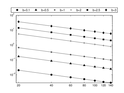
Figure 1. $\|e\|_{1,p(\cdot)}$ respect to $N^{1/2}$ in loglog scale

Fitting these values by the model $\|e\|_{1,p(\cdot)}\sim CN^{\nicefrac{{-\alpha}}{{2}}}$ using least square approximation gives us the results of Table 2.

$b$	$p_{1}$	$\alpha$	$C$
0.1	1.83	0.9984	0.1992
0.5	1.5	0.9961	1.6842
1	1.33	0.9900	6.52289
2	1.2	0.9998	55.3856
2.5	1.16	1.0007	143.9890
3	1.14	0.9495	329.2832

Table 2. Numerical order

Observe that the numerical rate of convergence is still of order one.

We also observe that $p_{1}$ is close to one when $b>>1$, for example $p_{1}=1.14$ if $b=3$. Table 2 shows that the constant $C$ increases when $p_{1}$ is near to one. In fact, the bound of the $\|u\|_{H^{2}(\Omega)}$ and the constants $C_{1}$ and $C_{2}$ in Lemma 2.1 depend on $\nicefrac{{1}}{{(p_{1}-1)}}$, see [1, 7].

References

[1]
John W. Barrett and W. B. Liu, Finite element approximation of the
-Laplacian, Math. Comp. 61 (1993), no. 204, 523–537.
MR 1192966 (94c:65129)
[2]
Erik M. Bollt, Rick Chartrand, Selim Esedoḡlu, Pete Schultz, and Kevin R.
Vixie, Graduated adaptive image denoising: local compromise between
total variation and isotropic diffusion, Adv. Comput. Math. 31
(2009), no. 1-3, 61–85.
[3]
Erich Carelli, Jonas Haehnle, and Andreas Prohl, Convergence analysis for
incompressible generalized Newtonian fluid flows with nonstandard
anisotropic growth conditions, SIAM J. Numer. Anal. 48 (2010),
no. 1, 164–190.
[4]
Yunmei Chen, Stacey Levine, and Murali Rao, Variable exponent, linear
growth functionals in image restoration, SIAM J. Appl. Math. 66
(2006), no. 4, 1383–1406 (electronic).
[5]
Ph. Ciarlet, The finite element method for elliptic problems, vol. 68,
North-Holland, Amsterdam, 1978.
[6]
Leandro M. Del Pezzo, Ariel L. Lombardi, and Sandra Martínez,
Interior penalty discontinuous Galerkin FEM for the
-Laplacian, SIAM J. Numer. Anal. 50 (2012), no. 5,
2497–2521. MR 3022228
[7]
Leandro M. Del Pezzo and Sandra Martínez, regularity for
the -Laplacian in two-dimensional convex domains, J. Math. Anal.
Appl. 410 (2014), no. 2, 939–952. MR 3111880
[8]
L. Diening, Theoretical and numerical results for electrorheological
fluids, Ph.D. thesis, Institut für Angewandte Mathematik, Mathematische
Fakultät, 7 2002.
[9]
by same author, Maximal function on generalized Lebesgue spaces
, Math. Inequal. Appl. 7 (2004), no. 2, 245–253.
MR 2057643 (2005k:42048)
[10]
Lars Diening, Petteri Harjulehto, Peter Hästö, and Michael
Ružička, Lebesgue and Sobolev spaces with
variable exponents, Lecture Notes in Mathematics, vol. 2017, Springer,
Heidelberg, 2011. MR 2790542
[11]
Lars Diening, Peter Hästö, and Aleš Nekvinda, Open problems
in variable exponent lebesgue and sobolev spaces, P. Drábek, J.
Rákosnık, FSDONA04 Proceedings, Milovy, Czech Republic (2004), 38–58.
[12]
Carsten Ebmeyer and WB. Liu, Quasi-norm interpolation error estimates for
the piecewise linear finite element approximation of -Laplacian
problems, Numer. Math. 100 (2005), no. 2, 233–258.
[13]
D. Gilbarg and N. S. Trudinger, Elliptic partial differential equations
of second order, Grundlehren der Mathematischen Wissenschaften [Fundamental
Principles of Mathematical Sciences], vol. 224, Springer-Verlag, Berlin,
1983.
[14]
Roland Glowinski, Numerical methods for nonlinear variational problems,
Scientific Computation, Springer-Verlag, Berlin, 2008, Reprint of the 1984
original. MR 2423313 (2009c:65002)
[15]
Kováčik and Rákosník, On spaces and
, Czechoslovak Math. J 41 (1991), 592–618.
[16]
W. B. Liu and John W. Barrett, A further remark on the regularity of the
solutions of the -Laplacian and its applications to their finite
element approximation, Nonlinear Anal. 21 (1993), no. 5, 379–387.
MR 1237129 (94h:35027)
[17]
by same author, A remark on the regularity of the solutions of the
-Laplacian and its application to their finite element approximation,
J. Math. Anal. Appl. 178 (1993), no. 2, 470–487. MR 1238889
(95a:35016)
[18]
Andreas Prohl and Weindl Isabelle, Convergence of an implicit finite
element discretization for a class of parabolic equations with nonstandard
anisotropic growth conditions, http://na.uni-tuebingen.de/preprints.shtml
(2007).
[19]
Michael Ružička, Electrorheological fluids:
modeling and mathematical theory, Lecture Notes in Mathematics, vol. 1748,
Springer-Verlag, Berlin, 2000.
[20]
S. Samko, Denseness of in the
generalized Sobolev spaces , Direct and
inverse problems of mathematical physics (Newark, DE, 1997), Int. Soc.
Anal. Appl. Comput., vol. 5, Kluwer Acad. Publ., Dordrecht, 2000,
pp. 333–342.