Exact Electronic Potentials in Coupled Electron-Ion Dynamics

Abstract

We develop a novel approach to the coupled motion of electrons and ions that focuses on the dynamics of the electronic subsystem. Usually the description of electron dynamics involves an electronic Schrödinger equation where the nuclear degrees of freedom appear as parameters or as classical trajectories. Here we derive the exact Schrödinger equation for the subsystem of electrons, staying within a full quantum treatment of the nuclei. This exact Schrödinger equation features a time-dependent potential energy surface for electrons (e-TDPES). We demonstrate that this exact e-TDPES differs significantly from the electrostatic potential produced by classical or quantum nuclei.

The theoretical description of electronic motion in the time domain is among the biggest challenges in theoretical physics. A variety of tools has been developed to tackle this problem, among them the Kadanoff-Baym approach Stefanucci and van Leeuwen (2013); *marini, time-dependent density functional theory Runge and Gross (1984); *carsten; *BSIN, the hierarchical equations of motion approach Jin et al. (2008); *chen as well as the multiconfiguration time-dependent Hartree-Fock approach Caillat et al. (2005); *kato; *WWCTR; *irene. From the point of view of electronic dynamics all these approaches are formally exact as long as the nuclei are considered clamped. However, some of the most fascinating phenomena result from the coupling of electronic and nuclear motion, e.g., photovoltaics  Rozzi et al. (2013); *DP07, processes in vision E.Tapavicza et al. (2007); *Polli, photosynthesis Tapavicza et al. (2011), molecular electronics Horsfield et al. (2004); *VSC; *Ratner, and strong field processes Zuo and Bandrauk (1995); *Esa; *Lein. To properly capture electron dynamics in these phenomena, it is essential to account for electron-nuclear (e-n) coupling.

In principle, the e-n dynamics is described by the complete time-dependent Schrödinger equation (TDSE)

$$\hat{H}\Psi({\underline{\underline{\bf r}}},{\underline{\underline{\bf R}}},t)=i\partial_{t}\Psi({\underline{\underline{\bf r}}},{\underline{\underline{\bf R}}},t),$$ (1)

with Hamiltonian

$$\hat{H}=\hat{T}_{n}({\underline{\underline{\bf R}}})+\hat{V}^{n}_{ext}({\underline{\underline{\bf R}}},t)+\hat{H}_{\rm BO}({\underline{\underline{\bf r}}},{\underline{\underline{\bf R}}})+\hat{v}^{e}_{ext}({\underline{\underline{\bf r}}},t),$$ (2)

where $\hat{H}_{\rm BO}({\underline{\underline{\bf r}}},{\underline{\underline{\bf R}}})$ is the traditional Born-Oppenheimer (BO) electronic Hamiltonian,

$$\hat{H}_{\rm BO}=\hat{T}_{e}({\underline{\underline{\bf r}}})+\hat{W}_{ee}({\underline{\underline{\bf r}}})+\hat{W}_{en}({\underline{\underline{\bf r}}},{\underline{\underline{\bf R}}})+\hat{W}_{nn}({\underline{\underline{\bf R}}}).$$ (3)

Here $\hat{T}_{n}=-\sum_{\alpha=1}^{N_{n}}\frac{\nabla^{2}_{\alpha}}{2M_{\alpha}}$ and $\hat{T}_{e}=-\sum_{j=1}^{N_{e}}\frac{\nabla^{2}_{j}}{2m}$ are the nuclear and electronic kinetic energy operators, $\hat{W}_{ee}$, $\hat{W}_{en}$ and $\hat{W}_{nn}$ are the electron-electron, e-n and nuclear-nuclear interaction, and $\hat{V}^{n}_{ext}({\underline{\underline{\bf R}}},t)$ and $\hat{v}^{e}_{ext}({\underline{\underline{\bf r}}},t)$ are time-dependent (TD) external potentials acting on the nuclei and electrons, respectively. Throughout this paper ${\underline{\underline{\bf R}}}$ and ${\underline{\underline{\bf r}}}$ collectively represent the nuclear and electronic coordinates respectively and $\hbar=1$.

A full numerical solution of the complete e-n TDSE, Eq. (1), is extremely hard to achieve and has been obtained only for small systems with very few degrees of freedom, such as H${}_{2}^{+}$ Chelkowski et al. (1995). For larger systems, an efficient and widely used approximation is the mixed quantum-classical description where the electrons are propagated quantum mechanically according to the TDSE

$$\Bigl{(}\hat{T}_{e}({\underline{\underline{\bf r}}})+\hat{W}_{ee}({\underline{\underline{\bf r}}})+V({\underline{\underline{\bf r}}},t)+\hat{v}^{e}_{ext}({\underline{\underline{\bf r}}},t)\Bigr{)}\Phi({\underline{\underline{\bf r}}},t)=i\partial_{t}\Phi({\underline{\underline{\bf r}}},t),$$ (4)

which is coupled to the classical nuclear trajectories, ${\bf R}_{\alpha}(t)$, determined by Ehrenfest or surface-hopping algorithms Tully (1998). The potential $V({\underline{\underline{\bf r}}},t)$ felt by the electrons is then given by the classical expression

$$V_{class}({\underline{\underline{\bf r}}},t)=W_{en}({\underline{\underline{\bf r}}},{\underline{\underline{\bf R}}}(t))=-\sum_{j=1}^{N_{e}}\sum_{\alpha=1}^{N_{n}}\frac{eZ_{\alpha}}{|{\bf r}_{j}-{\bf R}_{\alpha}(t)|},$$ (5)

where ${\underline{\underline{\bf R}}}(t)$ denotes the set of classical nuclear trajectories, ${\bf R}_{\alpha}(t)$. A better approximation to the potential $V({\underline{\underline{\bf r}}},t)$ felt by the electrons is the electrostatic or Hartree expression Tully (1998):

$$V_{\rm Hartree}({\underline{\underline{\bf r}}},t)=-eZ_{\alpha}\sum_{j=1}^{N_{e}}\sum_{\alpha=1}^{N_{n}}\int d{\underline{\underline{\bf R}}}\frac{|\chi({\underline{\underline{\bf R}}},t)|^{2}}{|{\bf r}_{j}-{\bf R}_{\alpha}|}\;$$ (6)

where $\chi({\underline{\underline{\bf R}}},t)$ represents a nuclear many-body wavefunction obtained, e.g., from nuclear wave packet dynamics. Clearly, Eq. (6) reduces to the classical expression (5) in the limit of very narrow wave packets centered around the classical trajectories ${\underline{\underline{\bf R}}}(t)$. The Hartree expression (6) incorporates the nuclear charge distribution, but the potential is still approximate as it neglects e-n correlations.

In this paper we address the question whether the potential $V({\underline{\underline{\bf r}}},t)$ in the purely electronic many-body TDSE, Eq. (4), can be chosen such that the resulting electronic wavefunction $\Phi({\underline{\underline{\bf r}}},t)$ becomes exact. By exact we mean that $\Phi({\underline{\underline{\bf r}}},t)$ reproduces the true electronic $N_{e}$-body density and the true $N_{e}$-body current density that would be obtained from the full e-n wavefunction $\Psi({\underline{\underline{\bf r}}},{\underline{\underline{\bf R}}},t)$ of Eq. (1). We shall demonstrate that the answer is yes provided we allow for a vector potential, ${\bf S}({\underline{\underline{\bf r}}},t)$, in the electronic TDSE, in addition to the scalar potential $V({\underline{\underline{\bf r}}},t)$. We will analyse this potential for an exciting experiment, namely the laser-induced localization of the electron in the H${}_{2}^{+}$ molecule Sansone et al. (2010); *HRB; *KSIV. We find significant differences between this exact potential and both the classical-nuclei potential Eq. (5) and the Hartree potential Eq. (6).

Refs. Abedi et al. (2010, 2012) proved that the exact solution of the complete molecular TDSE Eq. (1) can be written as a single product,

$$\Psi({\underline{\underline{\bf r}}},{\underline{\underline{\bf R}}},t)=\Phi_{{\underline{\underline{\bf R}}}}({\underline{\underline{\bf r}}},t)\chi({\underline{\underline{\bf R}}},t),$$ (7)

of a nuclear wavefunction $\chi({\underline{\underline{\bf R}}},t)$, and an electronic wavefunction parametrized by the nuclear coordinates, $\Phi_{{\underline{\underline{\bf R}}}}({\underline{\underline{\bf r}}},t)$, which satisfies the partial normalization condition (PNC) $\int d{\underline{\underline{\bf r}}}|\Phi_{{\underline{\underline{\bf R}}}}({\underline{\underline{\bf r}}},t)|^{2}=1$. Here we instead consider the reverse factorization,

$$\Psi({\underline{\underline{\bf r}}},{\underline{\underline{\bf R}}},t)=\chi_{{\underline{\underline{\bf r}}}}({\underline{\underline{\bf R}}},t)\Phi({\underline{\underline{\bf r}}},t)\;.$$ (8)

It is straightforward to see that the formalism presented in Ref. Abedi et al. (2010) follows through simply with a switch of the role of electronic and nuclear coordinates. In particular,

(i) The exact solution of the TDSE may be written as Eq. (8), where $\chi_{{\underline{\underline{\bf r}}}}({\underline{\underline{\bf R}}},t)$ satisfies the PNC $\int d{\underline{\underline{\bf R}}}|\chi_{{\underline{\underline{\bf r}}}}({\underline{\underline{\bf R}}},t)|^{2}=1$.

(ii) The nuclear wavefunction $\chi_{{\underline{\underline{\bf r}}}}({\underline{\underline{\bf R}}},t)$ satisfies

$$\Bigl{(}\hat{H}_{n}({\underline{\underline{\bf R}}},{\underline{\underline{\bf r}}},t)-\epsilon_{e}({\underline{\underline{\bf r}}},t)\Bigr{)}\chi_{{\underline{\underline{\bf r}}}}({\underline{\underline{\bf R}}},t)\\ =i\partial_{t}\chi_{{\underline{\underline{\bf r}}}}({\underline{\underline{\bf R}}},t),$$ (9)

with the nuclear Hamiltonian

$$\begin{split}\hat{H}_{n}&({\underline{\underline{\bf R}}},{\underline{\underline{\bf r}}},t)=\hat{T}_{n}({\underline{\underline{\bf R}}})+\hat{W}_{ee}({\underline{\underline{\bf r}}})+\hat{W}_{en}({\underline{\underline{\bf r}}},{\underline{\underline{\bf R}}})+\hat{W}_{nn}({\underline{\underline{\bf R}}})\\ &+\hat{v}_{\rm ext}^{e}({\underline{\underline{\bf r}}},t)+\hat{V}_{\rm ext}^{n}({\underline{\underline{\bf R}}},t)+\sum_{j=1}^{N_{e}}\frac{1}{m}\Big{[}\frac{(-i\nabla_{j}-{\bf S}_{j}({\underline{\underline{\bf r}}},t))^{2}}{2}\\ &+\Big{(}\frac{-i\nabla_{j}\Phi}{\Phi}+{\bf S}_{j}({\underline{\underline{\bf r}}},t)\Big{)}\left(-i\nabla_{j}-{\bf S}_{j}({\underline{\underline{\bf r}}},t)\right)\Big{]}.\end{split}$$ (10)

The electronic wavefunction $\Phi({\underline{\underline{\bf r}}},t)$ satisfies the TDSE:

$$\Bigl{(}\sum_{j=1}^{N_{e}}\frac{1}{2m}(-i\nabla_{j}+{\bf S}_{j}({\underline{\underline{\bf r}}},t))^{2}+\epsilon_{e}({\underline{\underline{\bf r}}},t)\Bigr{)}\Phi({\underline{\underline{\bf r}}},t)=i\partial_{t}\Phi({\underline{\underline{\bf r}}},t).$$ (11)

Here the exact TD potential energy surface for electrons (e-TDPES) $\epsilon_{e}({\underline{\underline{\bf r}}},t)$ and the exact electronic TD vector potential ${\bf S}_{j}({\underline{\underline{\bf r}}},t)$ are defined as

$$\epsilon_{e}({\underline{\underline{\bf r}}},t)=\left\langle\chi_{{\underline{\underline{\bf r}}}}(t)\right|\hat{H}_{n}({\underline{\underline{\bf R}}},{\underline{\underline{\bf r}}},t)-i\partial_{t}\left|\chi_{{\underline{\underline{\bf r}}}}(t)\right\rangle_{\underline{\underline{\bf R}}}$$ (12)

$${\bf S}_{j}({\underline{\underline{\bf r}}},t)=\left\langle\chi_{{\underline{\underline{\bf r}}}}(t)\right|\left.-i\nabla_{j}\chi_{\underline{\underline{\bf r}}}(t)\right\rangle_{\underline{\underline{\bf R}}}$$ (13)

where $\langle...|...|...\rangle_{\underline{\underline{\bf R}}}$ denotes an inner product over all nuclear variables only.

(iii) Eqs. (9)- (11) are form-invariant under the following gauge-like transformation $\chi_{{\underline{\underline{\bf r}}}}({\underline{\underline{\bf R}}},t)\rightarrow\tilde{\chi}_{{\underline{\underline{\bf r}}}}({\underline{\underline{\bf R}}},t)=\exp(i\theta({\underline{\underline{\bf r}}},t))\chi_{{\underline{\underline{\bf r}}}}({\underline{\underline{\bf R}}},t)$, $\Phi({\underline{\underline{\bf r}}},t)\rightarrow\tilde{\Phi}({\underline{\underline{\bf r}}},t)=\exp(-i\theta({\underline{\underline{\bf r}}},t))\Phi({\underline{\underline{\bf r}}},t)$, while the potentials transform as ${\bf S}_{j}({\underline{\underline{\bf r}}},t)\rightarrow\tilde{\bf S}_{j}({\underline{\underline{\bf r}}},t)={\bf S}_{j}({\underline{\underline{\bf r}}},t)+\nabla_{j}\theta({\underline{\underline{\bf r}}},t)$, $\epsilon_{e}({\underline{\underline{\bf r}}},t)\rightarrow\tilde{\epsilon}_{e}({\underline{\underline{\bf r}}},t)=\epsilon_{e}({\underline{\underline{\bf r}}},t)+\partial_{t}\theta({\underline{\underline{\bf r}}},t)$. The wave functions $\chi_{{\underline{\underline{\bf r}}}}({\underline{\underline{\bf R}}},t)$ and $\Phi({\underline{\underline{\bf r}}},t)$ yielding a given solution, $\Psi({\underline{\underline{\bf r}}},{\underline{\underline{\bf R}}},t)$, of Eq. (1) are unique up to this $({\underline{\underline{\bf r}}},t)$-dependent phase transformation.

(iv) The wave functions $\chi_{{\underline{\underline{\bf r}}}}({\underline{\underline{\bf R}}},t)$ and $\Phi({\underline{\underline{\bf r}}},t)$ are interpreted as nuclear and electronic wavefunctions: $|\Phi({\underline{\underline{\bf r}}},t)|^{2}=\int|\Psi({\underline{\underline{\bf r}}},{\underline{\underline{\bf R}}},t)|^{2}d{\underline{\underline{\bf R}}}$ is the probability density of finding the electronic configuration ${\underline{\underline{\bf r}}}$ at time $t$, and $|\chi_{{\underline{\underline{\bf r}}}}({\underline{\underline{\bf R}}},t)|^{2}=|\Psi({\underline{\underline{\bf r}}},{\underline{\underline{\bf R}}},t)|^{2}/|\Phi({\underline{\underline{\bf r}}},t)|^{2}$ is the conditional probability of finding the nuclei at ${\underline{\underline{\bf R}}}$, given that the electronic configuration is ${\underline{\underline{\bf r}}}$. The exact electronic $N_{e}$-body current-density can be obtained from ${\rm Im}(\Phi^{*}\nabla_{j}\Phi)+|\Phi({\underline{\underline{\bf r}}},t)|^{2}{\bf S}_{j}$.

We can regard Eq. (11) as the exact electronic TDSE: The time evolution of $\Phi({\underline{\underline{\bf r}}},t)$ is completely determined by the exact e-TDPES, $\epsilon_{e}({\underline{\underline{\bf r}}},t)$, and the vector potential ${\bf S}_{j}({\underline{\underline{\bf r}}},t)$. Moreover, these potentials are unique up to within a gauge transformation (iii, above). In other words, if one requires a purely electronic TDSE (11) with solution $\Phi({\underline{\underline{\bf r}}},t)$ to yield the true electron ($N_{e}$-body) density and current density of the full e-n problem, then the potentials appearing in this TDSE are (up to within a gauge transformation) uniquely given by Eqs. (12) and (13).

A formalism in which the nuclear wavefunction is conditionally dependent on the electronic coordinates, rather than the other way around, may appear somewhat non-intuitive. However, in many non-adiabatic processes, the nuclear and electronic speeds are comparable, and, in some cases, such as highly excited Rydberg molecules, nuclei may even move faster than electrons Rabani and Levine (1996). We shall show in the following that the present factorization is useful to interpret the dynamics of attosecond electron localization, and that it gives direct insight into how the e-n coupling affects non-adiabatic electron dynamics. For this purpose it is useful to rewrite the exact e-TDPES as

$$\epsilon_{e}({\underline{\underline{\bf r}}},t)=\epsilon^{\rm approx}_{e}({\underline{\underline{\bf r}}},t)+\Delta\epsilon_{e}({\underline{\underline{\bf r}}},t)$$ (14)

where

$$\begin{split}\epsilon^{\rm approx}_{e}({\underline{\underline{\bf r}}},t)&=\left\langle\chi_{\underline{\underline{\bf r}}}(t)\right|\hat{W}_{ee}({\underline{\underline{\bf r}}})+\hat{W}_{en}({\underline{\underline{\bf r}}},{\underline{\underline{\bf R}}})+\hat{W}_{nn}({\underline{\underline{\bf R}}})\\ &+\hat{v}^{e}_{ext}({\underline{\underline{\bf r}}},t)+\hat{V}^{n}_{ext}({\underline{\underline{\bf R}}},t)\left|\chi_{\underline{\underline{\bf r}}}(t)\right\rangle_{\underline{\underline{\bf R}}}\end{split}$$ (15)

and

$$\begin{split}\Delta\epsilon_{e}({\underline{\underline{\bf r}}},t)&=\left\langle\chi_{{\underline{\underline{\bf r}}}}(t)\right|\hat{T}_{n}({\underline{\underline{\bf R}}})\left|\chi_{{\underline{\underline{\bf r}}}}(t)\right\rangle_{\underline{\underline{\bf R}}}+\left\langle\chi_{{\underline{\underline{\bf r}}}}(t)\right|-i\partial_{t}\left|\chi_{{\underline{\underline{\bf r}}}}(t)\right\rangle_{\underline{\underline{\bf R}}}\\ &+\sum_{j=1}^{N_{e}}\frac{\left\langle\nabla_{j}\chi_{{\underline{\underline{\bf r}}}}(t)|\nabla_{j}\chi_{{\underline{\underline{\bf r}}}}(t)\right\rangle_{\underline{\underline{\bf R}}}}{2m}-\sum_{j=1}^{N_{e}}\frac{{\bf S}^{2}_{j}({\underline{\underline{\bf r}}},t)}{2m}.\end{split}$$ (16)

If the nuclear density is approximated as a delta-function at ${\underline{\underline{\bf R}}}(t)$, then $\epsilon^{\rm approx}_{e}$ reduces to the electronic potential used in the traditional mixed quantum-classical approximations:

$$\begin{split}\epsilon^{\rm trad}_{e}({\underline{\underline{\bf r}}},t)=&\hat{W}_{ee}({\underline{\underline{\bf r}}})+\hat{W}_{en}({\underline{\underline{\bf r}}},{\underline{\underline{\bf R}}}(t))+\hat{W}_{nn}({\underline{\underline{\bf R}}}(t))\\ &+\hat{v}^{e}_{ext}({\underline{\underline{\bf r}}},t)+\hat{V}^{n}_{ext}({\underline{\underline{\bf R}}}(t)).\end{split}$$ (17)

This approximation not only neglects the width of the nuclear wavefunction but it also misses the contribution to the potential from $\Delta\epsilon_{e}({\underline{\underline{\bf r}}},t)$, Eq. (16). Methods that retain a quantum description of the nuclei (e.g. TD Hartree  Tully (1998)) approximate Eq. (15), although without the parametric dependence of the nuclear wavefunction on ${\underline{\underline{\bf r}}}$, and still miss the contribution from Eq. (16). In the following example, we will show the significance of the e-n correlation represented in the term $\Delta\epsilon_{e}$.

Among the many charge-transfer processes accompanying nuclear motion mentioned earlier, here we study attosecond electron localization dynamics in the dissociation of the H${}_{2}^{+}$ molecule achieved by time-delayed coherent ultrashort laser pulses Sansone et al. (2010); *HRB; *KSIV. In the experiment, first an ultraviolet (UV) pulse excites H${}_{2}^{+}$ to the dissociative $2p\sigma_{u}$ state while a second time-delayed infrared (IR) pulse induces electron transfer between the dissociating atoms. This relatively recent technique has gathered increasing attention since it is expected to eventually lead to the direct control of chemical reactions via the control of electron dynamics. Extensive theoretical studies have led to progress in understanding the mechanism Sansone et al. (2010); *HRB; *KSIV, and highlight the important role of e-n correlated motion. Here we study the exact e-n coupling terms by computing the exact e-TDPES Eq. (12).

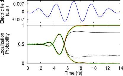
Figure 1: Electron localization probabilities along the negative (solid line) and the positive z-axis (dashed line) as a function of time, obtained from exact dynamics (black), dynamics on the traditional potential $\epsilon^{\rm trad}_{e}$ evaluated at the exact mean nuclear position (red), and dynamics on the approximate potential $\epsilon^{\rm approx}_{e}$ (green). The field is shown in the top panel.

We consider a one-dimensional H${}_{2}^{+}$ model, starting the dynamics after the excitation by the UV pulse: the wavepacket starts at $t=0$ on the first excited state ($2p\sigma_{u}$ state) of H${}_{2}^{+}$ as a Frank-Condon projection of the wavefunction of the ground state, and then is exposed to the IR laser pulse. The Hamiltonian is given by Eq. (2), with ${\underline{\underline{\bf R}}}\to R$, the internuclear distance, and ${\underline{\underline{\bf r}}}\to z$, the electronic coordinate as measured from the nuclear center-of mass . The kinetic energy terms are $\hat{T}_{n}(R)=-\frac{1}{2\mu_{n}}\frac{\partial^{2}}{\partial R^{2}}$ and, $\hat{T}_{e}(z)=-\frac{1}{2\mu_{e}}\frac{\partial^{2}}{\partial z^{2}}$, respectively, where the reduced mass of the nuclei is given by $\mu_{n}=M_{\rm H}/2$, and reduced electronic mass is given by $\mu_{e}=\frac{2M_{\rm H}}{2M_{\rm H}+1}$ ($M_{\rm H}$ is the proton mass). The interactions are soft-Coulomb: $\hat{W}_{nn}(R)=\frac{1}{\sqrt{0.03+R^{2}}}$, and $\hat{W}_{en}(z,R)=-\frac{1}{\sqrt{1.0+(z-\frac{R}{2})^{2}}}-\frac{1}{\sqrt{1.0+(z+\frac{R}{2})^{2}}}$ (and $\hat{W}_{ee}=0$). The IR pulse is taken into account using the dipole approximation and length gauge, as $\hat{v}^{e}_{ext}(z,t)=E(t)q_{e}z$, where $E(t)=E_{0}\exp\left[-\left(\frac{t-\Delta t}{\tau}\right)^{2}\right]\cos(\omega(t-\Delta t))$, and the reduced charge $q_{e}=\frac{2M_{\rm H}+2}{2M_{\rm H}+1}$. The wavelength is 800 nm and the peak intensity $I_{0}=E_{0}^{2}=3.0\times 10^{12}$W/cm². The pulse duration is $\tau=4.8fs$ and $\Delta t$ is the time delay between the UV and IR pulses. Here we show the results of $\Delta t=$ 7 fs. We propagate the full TDSE (1) numerically exactly to obtain the full molecular wavefunction $\Psi(z,R,t)$, and from it we calculate the probabilities of directional localization of the electron, $P_{\pm}$, which are defined as $P_{+(-)}=\int_{z>(<)0}dz\int dR|\Psi(z,R,t)|^{2}$. These are shown as the black solid ($P_{-}$) and dashed ($P_{+}$) lines in Fig. 1. It is evident from this figure that considerable electron localization occurs, with the electron density predominantly localized on the left (negative z-axis).

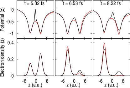
Figure 2: Top panel: Electronic potentials at the times indicated: (exact $\epsilon_{e}$ (black), traditional $\epsilon^{\rm trad}_{e}$ evaluated at the exact mean nuclear position (red)). Lower panel: Electron densities obtained from dynamics on the electronic potentials shown in the top panel.

We now propagate the electrons under the traditional potential Eq. (17), employing the exact TD mean nuclear position $R(t)$ obtained from $\Psi(z,R,t)$ by $R(t)=\left\langle\Psi(z,R,t)\right|R\left|\Psi(z,R,t)\right\rangle$, and calculate the electron localization probabilities, shown as red solid line (negative region) and dashed line (positive region) in Fig. 1. Comparing the red and black lines in Fig. 1, we find that the traditional potential yields the correct dynamics until around 5 fs, but then becomes less accurate: finally it predicts the electron to be almost perfectly localized on the left nucleus, while the exact calculation still gives some probability of finding the electron on the right.

To understand the error in the dynamics determined by the traditional surface, we compute the exact e-TDPES (12) in the gauge where the vector potential $S(z,t)$ is zero . In the upper panel of Fig. 2, the exact $\epsilon_{e}$ (Eq. (12)) is plotted (black line) at three times  , and compared with the traditional potential (Eq. (17)) $\epsilon^{\rm trad}_{e}$ (red line) evaluated at the exact mean nuclear position. In the lower panel, the electron densities calculated from dynamics on the respective potentials are plotted.

A notable difference between $\epsilon_{e}$ and $\epsilon^{\rm trad}_{e}$ is an additional interatomic barrier which appears in the exact potential, and a step-like feature that shifts one well with respect to the other. These additional features arise from the coupling terms contained in $\Delta\epsilon$, and are responsible for the correct dynamics, which is evident from the green curve in Fig. 1: this shows the results predicted by propagating the electrons on $\epsilon^{\rm approx}_{e}$. The result is close to that of the red traditional curve, and the potentials (not shown for figure clarity) are also close to the red potentials shown in Fig  2. A TD Hartree treatment is also close to the results from propagating on $\epsilon^{\rm trad}_{e}$. An examination of the different components in Eq. (16) shows that the additional interatomic barrier arises from the term $\frac{1}{2m}\left\langle\frac{\partial}{\partial z}\chi_{z}|\frac{\partial}{\partial z}\chi_{z}\right\rangle_{R}$, while the other two terms in Eq. (16) yield the step.

The current understanding of the mechanism for electron localization is that as the molecule dissociates, there is a rising interatomic barrier from $W_{en}$, which, when it reaches the energy level of the excited electronic state largely shuts off electron transfer between the ions Sansone et al. (2010); *HRB; *KSIV. The electron distribution is largely frozen after this point, as the electron can only tunnel between the nuclei. The additional barrier we see in the exact e-TDPES, leads to an earlier localization time, and ultimately smaller localization asymmetry. However, each of the three terms in Eq. (16) for $\Delta\epsilon$ play an important role in the dynamics: if the electronic system is evolved adding only the barrier correction to $\epsilon^{\rm approx}_{e}$ the localization asymmetry is somewhat reduced compared to evolving on $\epsilon^{\rm approx}_{e}$ alone but far more so when all three terms of $\Delta\epsilon$ are included.

In conclusion, we have presented the exact factorization of the complete molecular wavefunction into electronic and nuclear wavefunctions, $\Psi({\underline{\underline{\bf r}}},{\underline{\underline{\bf R}}},t)=\chi_{\underline{\underline{\bf r}}}({\underline{\underline{\bf R}}},t)\Phi({\underline{\underline{\bf r}}},t)$, where the electronic wavefunction $\Phi({\underline{\underline{\bf r}}},t)$ satisfies an electronic TDSE, and the nuclear wavefunction is conditionally dependent on the electronic coordinates. This is complementary to the factorization of Refs. Abedi et al. (2010, 2012, 2013), $\Psi({\underline{\underline{\bf r}}},{\underline{\underline{\bf R}}},t)=\chi({\underline{\underline{\bf R}}},t)\Phi_{\underline{\underline{\bf R}}}({\underline{\underline{\bf r}}},t)$, where instead the nuclear wavefunction satisfies a TDSE while the electronic wavefunction does not. The exact e-TDPES and exact TD vector potential acting on the electrons were uniquely defined and compared with the traditional potentials used in studying localization dynamics in a model of the H${}_{2}^{+}$ molecular ion. The importance of the exact e-n correlation in the e-TDPES in reproducing the correct electron dynamics was demonstrated. Further studies on this and other model systems will lead to insight into how e-n correlation affects electron dynamics in non-adiabatic processes, an insight that can never be gained from the classical electrostatic potentials caused by the point charges of the clamped nucleus nor the charge distributions of the exact nuclear density. Preliminary studies using the Shin-Metiu model Shin and Metiu (1995) of field-free electronic dynamics in the presence of strong non-adiabatic couplings show that peak and shift structures in the exact e-TDPES, similar to those in the localization problem discussed here, appear typically after non-adiabatic transitions. Finally, we note that the exact TD electronic potentials defined in this study, together with the exact TD nuclear potentials derived in Abedi et al. (2010, 2012) establish the exact potential functionals of TD multicomponent density functional theory Li and Tong (1986); Kreibich et al. (2008); Kreibich and Gross (2001). The study of these potentials may ultimately lead to approximate density-functionals for use in this theory, which holds promise for the description of real-time coupled e-n dynamics in real systems.

Partial support from the Deutsche Forschungsgemeinschaft (SFB 762), the European Commission (FP7-NMP-CRONOS), and the U.S. Department of Energy, Office of Basic Energy Sciences, Division of Chemical Sciences, Geosciences and Biosciences under award DE-SC0008623 (NTM),is gratefully acknowledged.

References

- Stefanucci and van Leeuwen (2013) G. Stefanucci and R. van Leeuwen, Nonequilibrium Many Body Theory of Quantum Systems: A Modern Introduction (Cambridge University Press, 2013).
- Attaccalite et al. (2011) C. Attaccalite, M. Grüning, and A. Marini, Phys. Rev. B 84, 245110 (2011).
- Runge and Gross (1984) E. Runge and E. K. U. Gross, Phys. Rev. Lett. 52, 997 (1984).
- Ullrich (2012) C. A. Ullrich, Time-Dependent Density-Functional Theory: Concepts and Applications (Oxford University Press, 2012).
- Baer et al. (2004) R. Baer, T. Seideman, S. Ilani, and D. Neuhauser, J. Chem. Phys. 120, 3387 (2004).
- Jin et al. (2008) J. S. Jin, X. Zheng, and Y. J. Yan, J. Chem. Phys. 128, 234703 (2008).
- Zheng et al. (2010) X. Zheng, G. H. Chen, Y. Mo, S. K. Koo, H. Tian, C. Y. Yam, and Y. J. Yan, J. Chem. Phys. 133, 114101 (2010).
- Caillat et al. (2005) J. Caillat, J. Zanghellini, M. Kitzler, O. Koch, W. Kreuzer, and A. Scrinzi, Phys. Rev. A 71, 012712 (2005).
- Kato and Kono (2008) T. Kato and H. Kono, J. Chem. Phys. 128, 184102 (2008).
- Wilner et al. (2013) E. Y. Wilner, H. Wang, G. Cohen, M. Thoss, and E. Rabani, Phys. Rev. B 88, 045137 (2013).
- Burghardt et al. (2008) I. Burghardt, K. Giri, and G. A. Worth, J. Chem. Phys. 129, 174104 (2008).
- Rozzi et al. (2013) C. A. Rozzi et al., Nature Comm. 4, 1602 (2013).
- Duncan and Prezhdo (2007) W. R. Duncan and O. V. Prezhdo, Annu. Rev. Phys. Chem. 58, 143 (2007).
- E.Tapavicza et al. (2007) E.Tapavicza, I. Tavernelli, and U. Rothlisberger, Phys. Rev. Lett. 98, 023001 (2007).
- Polli et al. (2010) D. Polli et al., Nature 467, 440 (2010).
- Tapavicza et al. (2011) E. Tapavicza, A. M. Meyer, and F. Furche, Phys. Chem. Chem. Phys. 13, 20986 (2011).
- Horsfield et al. (2004) A. P. Horsfield, D. R. Bowler, A. J. Fisher, T. N. Todorov, and M. J. Montgomery, J. Phys.: Condens. Matter 16, 3609 (2004).
- Verdozzi et al. (2006) C. Verdozzi, G. Stefanucci, and C.-O. Almbladh, Phys. Rev. Lett. 97, 046603 (2006).
- Nitzan and Ratner (2003) A. Nitzan and M. A. Ratner, Science 300, 1384 (2003).
- Zuo and Bandrauk (1995) T. Zuo and A. D. Bandrauk, Phys. Rev. A 52, R2511 (1995).
- Räsänen and Madsen (2012) E. Räsänen and L. B. Madsen, Phys. Rev. A 86, 033426 (2012).
- Henkel et al. (2011) J. Henkel, M. Lein, and V. Engel, Phys. Rev. A 83, 051401(R) (2011).
- Chelkowski et al. (1995) S. Chelkowski, T. Zuo, O. Atabek, and A. D. Bandrauk, Phys. Rev. A 52, 2977 (1995).
- Tully (1998) J. C. Tully, Faraday Discuss. 110, 407 (1998).
- Sansone et al. (2010) G. Sansone et al., Nature 465, 763 (2010).
- He et al. (2007) F. He, C. Ruiz, and A. Becker, Phys. Rev. Lett. 99, 083002 (2007).
- Kelkensberg et al. (2011) F. Kelkensberg, G. Sansone, M. Y. Ivanov, and M. Vrakking, Phys. Chem. Chem. Phys. 13, 8647 (2011).
- Abedi et al. (2010) A. Abedi, N. T. Maitra, and E. K. U. Gross, Phys. Rev. Lett. 105, 123002 (2010).
- Abedi et al. (2012) A. Abedi, N. T. Maitra, and E. K. U. Gross, J. Chem. Phys. 137, 22A530 (2012).
- Rabani and Levine (1996) E. Rabani and R. D. Levine, J. Chem. Phys. 104, 1937 (1996).
- Note (1) In this model system the electronic wavefunction and density are defined with respect to a coordinate frame attached to the nuclear framework so that they are characteristic for the internal properties of the system Kreibich et al. (2008); *KG.
- Note (2) In general, both the scalar e-TDPES (12) and the vector potential (13) are present. In our specific -example it is easy to see that the vector potential can be gauged away so that the e-TDPES remains as the only potential acting on the electronic subsystem.
- Note (3) In Fig. 2, curves representing have been rigidly shifted along the energy axis to compare with the traditional potentials.
- Abedi et al. (2013) A. Abedi, F. Agostini, Y. Suzuki, and E. K. U. Gross, Phys. Rev. Lett. 110, 263001 (2013).
- Shin and Metiu (1995) S. Shin and H. Metiu, J. Chem. Phys. 102, 9285 (1995).
- Li and Tong (1986) T.-C. Li and P.-Q. Tong, Phys. Rev. A 34, 529 (1986).
- Kreibich et al. (2008) T. Kreibich, R. van Leeuwen, and E. K. U. Gross, Phys. Rev. A 78, 022501 (2008).
- Kreibich and Gross (2001) T. Kreibich and E. K. U. Gross, Phys. Rev. Lett. 86, 2984 (2001).