Functional Renormalization Group Approach for Inhomogeneous Interacting Fermi-Systems

Abstract

The functional renormalization group (fRG) approach has the property that, in general, the flow equation for the two-particle vertex generates $\mathcal{O}(N^{4})$ independent variables, where $N$ is the number of interacting states (e.g. sites of a real-space discretization). In order to include the flow equation for the two-particle vertex one needs to make further approximations if $N$ becomes too large. We present such an approximation scheme, called the coupled-ladder approximation, for the special case of an onsite interaction. Like the generic third-order-truncated fRG, the coupled-ladder approximation is exact to second order and is closely related to a simultaneous treatment of the random phase approximation in all channels, i.e. summing up parquet-type diagrams. The scheme is applied to a one-dimensional model describing a quantum point contact.

I Introduction

The calculation of properties of an inhomogeneous interacting quantum system requires adequate care regarding a proper description of its spatial structure: for a lattice model the resolution of a potential landscape, without generating additional finite size effects, typically requires an extension of $\sim\!10^{2}$ sites per spatial dimension. If, in addition, the strength of interactions cannot be regarded as ‘weak’, a reasonable approximation scheme must involve detailed information about higher order correlations. This usually demands a huge effort for modern computers, both in memory and speed. Thus, for a system with non-trivial spatial structure any approximation scheme necessarily involves a tradeoff between computational feasibility and accuracy.

In Ref. Bauer et al., 2013, we introduced such a scheme, both reasonably fast and accurate up to intermediate interaction strength, within the framework of the one-particle irreducible version of the functional renormalization group (fRG).Wetterich (1993); Metzner et al. (2012); Meden et al. (2002); Andergassen et al. (2004, 2006); Karrasch et al. (2008); Karrasch (2006); Husemann et al. (2012); Giering and Salmhofer (2012) The goal of this paper is to supply a detailed description of this approximation scheme, called the coupled-ladder approximation (CLA), which is implemented within the context of generic, third-order-truncated fRG. In the latter, the flow of the three-particle vertex is set to zero, while the flow equation of the two-particle vertex (which we will call “vertex flow” in the following) is fully incorporated. This vertex flow has to be incorporated if interactions cannot be considered small. In general, this constitutes a computational challenge, since the vertex generated by this flow involves a large number $\mathcal{O}(N^{4})$ of independent functions, each depending on three frequencies, where $N$ is the number of sites of the interacting region. As a result, the flow equations involve $\mathcal{O}(N^{4}N_{\rm f}^{3})$ independent variables, where $N_{\rm f}$ is the number of discrete points per frequency used in the numerics. Previous schemes that included the vertex flow for models with large $N$ made use of an additional symmetry, e.g. Ref. Andergassen et al., 2004, 2006 described systems with a weak spatial inhomogeneity (either changing adiabatically with position, or confined to a small region), which could be treated as a perturbation, so that its feedback to the vertex could be neglected. The resulting equations for the vertex were solved in the momentum basis, exploiting the fact that the single-particle eigenstates could approximately be represented by plane waves. However, this is not possible for models with strong inhomogeneities. Our CLA scheme was developed to include the vertex flow for such models. It extends the idea of Refs. Karrasch et al., 2008 and Jakobs et al., 2010a, where the CLA was introduced to parametrize the frequency dependence of the vertex for the single-impurity Anderson model, i.e. $N=1$, which reduces the number of independent variables for that model to $\mathcal{O}(N_{\rm f})$. We show that the CLA can be applied to parametrize the spatial dependence of the vertex for models with a purely local interaction. The number of independent variables that represent the spatial dependence of the vertex then reduces to $\mathcal{O}(N^{2})$, and the total number of independent variables representing the vertex to $\mathcal{O}(N^{2}N_{\rm f})$. The CLA scheme is exact to second orderHonerkamp (2001); Honerkamp and Salmhofer (2003) and effectively sums up diagrams of the Random Phase Approximation (RPA) of all three interaction channels.

To illustrate the capabilities of our CLA scheme, we apply it, as in Ref. Bauer et al., 2013, to a one-dimensional chain modeling the lowest submode of a quantum point contact (QPC), a short constriction that allows transport only in one dimension. Its conductance is famously quantizedvan Wees et al. (1988); Wharam et al. (1988); Büttiker (1990) in units of $G_{Q}={2e^{2}}/{h}$. In addition to this quantization, measured conductance curves show a shoulder at around $0.7G_{Q}$. In this regime quantities such as electrical and thermal conductance, noise and thermo-power have anomalous behaviorThomas et al. (1996); Appleyard et al. (2000); Cronenwett et al. (2002). These phenomena are collectively known as the “0.7-anomaly” in QPCs.

In Ref. Bauer et al., 2013 we showed that the 0.7-anomaly is reproduced by a one-dimensional model with a parabolic potential barrier and a short-ranged Coulomb interaction. We presented a detailed microscopic picture that explained the physical mechanism which causes the anomalous behavior. Its origin is a smeared van Hove singularity in the density of states (DOS) just above the band bottom which enhances effects of interaction causing an enhanced backscattering. We presented detailed results for the conductance at zero temperature, obtained using fRG in the CLA. These numerical data were in good qualitative agreement with our experimental measurements and showed that the model reproduces the phenomenology of the 0.7-anomaly. In this paper we set forth and examine the approximation scheme in detail. We present additional numerical data to verify the reliability of the method for the case where it is applied to the model of a QPC. For this we present and compare data obtained by different approximation schemes within the fRG, showing that the phenomenology is very robust, and can even be obtained by neglecting the vertex flow. However including the vertex flow using the CLA reduces artifacts and gives an insightful view on the spin susceptibility. For the latter, we finally present a detailed quantitative error analysis.

II Microscopic Model

The approximation scheme presented in this paper can be applied to any model Hamiltonian that can be written in the following form:

$$H=\sum_{ij,\sigma}h_{ij}^{\sigma}d^{\dagger}_{i\sigma}d_{j\sigma}+\sum_{j}U_{j}n_{j\uparrow}n_{j\downarrow}\;,$$ (1)

where $h^{\sigma}$ is a real, symmetric matrix, $d^{\dagger}_{j\sigma}$ ($d_{j\sigma}$) creates (annihilates) an electron at site $j$ with spin $\sigma$ ($=\uparrow,\downarrow$ or $+,-$, with $\bar{\sigma}\!=\!-\sigma$), and $n_{j\sigma}=d^{\dagger}_{j\sigma}d_{j\sigma}$ counts them (in general $j$ can represent any quantum number, however for simplicity we refer to it as a site index throughout the paper). In order to apply the CLA the necessary property of this Hamiltonian is a short-ranged interaction. In principle the approximation scheme can be set up for an interaction with finite range (over several sites), however since the structure then becomes very complicated we will only discuss the case of a purely local, i.e., on-site interaction in this paper as given by Eq. (1). Whereas the system can extend to infinity, it is crucial that the number of sites $N$ where $U_{j}$ is nonzero is finite and not too large , as discussed in section III.8. If the system is extended to infinity, the effect of the noninteracting region can be calculated analytically using the projection method (see appendix Sec. A and Refs. Taylor, 1972 and Karrasch, 2006). An extension to a Hamiltonian that is complex Hermitian and non-diagonal in spin space, needed, e.g., to include spin-orbit effects, is straightforward. In contrast applying the scheme to spin less models, for which the interaction term has to be non-local to respect Pauli’s exclusion principle, is more complicated.

III fRG flow equations

In this section we describe the functional Renormalization Group (fRG) approach that we have employed to treat a translationally nonuniform Fermi system with onsite interactions, such as described by Eq. (1). We use the one-particle irreducible (1PI) version of the fRGWetterich (1993); Morris (1994). Its key idea is to approximately sum up a perturbative expansion, in our case in the interaction, by setting up and numerically solving a set of coupled ordinary differential equations (ODEs), the flow equations, for the system’s 1PI $n$-particle vertex functions, $\gamma_{n}$. This is typically done in such a way that the effects of higher-energy modes, lying above a flowing infrared cutoff parameter $\Lambda$, are incorporated before those of lower-energy modes lying below $\Lambda$. This yields a systematic way of summing up parquet-type diagrams for the two-particle vertex and for calculating the self-energy. $\Lambda$ serves as flow parameter that controls the RG flow of the $\Lambda$-dependent vertex functions $\gamma_{n}^{\Lambda}$ from an initial cutoff $\Lambda_{i}$, at which all vertex functions are known and simple, to a final cutoff $\Lambda_{f}$, at which the full theory is recovered.

This idea is implemented by replacing, in the generating functional for the vertex functions $\gamma_{n}$, the bare propagator $\mathcal{G}_{0}$ by a modified propagator $\mathcal{G}^{\Lambda}_{0}$,

$$\mathcal{G}_{0}\rightarrow\mathcal{G}_{0}^{\Lambda}\;,\quad\textrm{with}\quad\mathcal{G}_{0}^{\Lambda_{i}}=0,\quad\mathcal{G}_{0}^{\Lambda_{f}}=\mathcal{G}_{0}\;,$$ (2)

constructed such that $\mathcal{G}_{0}^{\Lambda}$ is strongly suppressed for frequencies below $\Lambda$. The $\Lambda$-dependence of the resulting vertex functions $\gamma_{n}^{\Lambda}$ is governed by an infinite hierarchy of coupled ODEs, the RG flow equations, of the form

$$\frac{d}{d\Lambda}\gamma^{\Lambda}_{n}=\mathcal{F}\left(\Lambda,\mathcal{G}^{\Lambda}_{0},\gamma^{\Lambda}_{1},\dots,\gamma^{\Lambda}_{n+1}\right)\;,$$ (3)

where $\gamma_{1}=-\Sigma$ is the self-energy and $\gamma_{2}$ the two particle vertex. At the beginning of the RG flow, the vertex functions are initialized to their bare values,

$$\gamma^{\Lambda_{i}}_{2}=v\quad\gamma^{\Lambda_{i}}_{n}=0\quad(n\neq 2),$$ (4)

while their fully dressed values, corresponding to the full theory, are recovered upon integrating Eqs. (3) from $\Lambda_{i}$ to $\Lambda_{f}$.

The infinite hierarchy of ODEs (3) is exact, but in most cases not solvable. In the generic, third-order-truncated fRG all $n$-particle vertex functions with $n\geq 3$ are neglected

$$\frac{d}{d\Lambda}\gamma_{n}=0\qquad(n\geq 3)\,,$$ (5)

and the resulting flow equations for $\gamma_{1}^{\Lambda}$ and $\gamma_{2}^{\Lambda}$ are integrated numerically. Due to this truncation, fRG is in essence an “RG-enhanced” perturbation expansion in the interaction, that will break down if $U$ becomes too large. In fact, the flow equations can be derived by a purely diagrammatic procedure, without resorting to a generating functional, as explained in Ref. Jakobs et al., 2007. The diagrammatic structure is such that the flow of the self-energy and three different parquet channels (i.e. three coupled RPA-like series of diagrams) are treated simultaneously, feeding into each other during the flow (as discussed in more detail below). This moderates competing instabilities in an unbiased way. We also mention that this approach has been found to be particularly useful to treat models where infrared divergences play a roleMetzner et al. (2012) (though the latter do not arise for the present model).

The following statements in this chapter hold for most, however not for every flow parameter. For that reason we explicitly define the $\Lambda$-dependence at this point. If a different fRG scheme is used, one should carefully check all relations. The general idea should be applicable for all fRG schemes. We use fRG in the Matsubara formalism. In the following frequencies with subscripts $n$, $n^{\prime}$, $n_{1}$, etc., are defined to be purely imaginary:

$$\omega_{n}=iT\pi(2n+1).$$ (6)

We introduce $\Lambda$ as an infrared cutoff in the bare Matsubara propagator,

$$\mathcal{G}_{0}^{\Lambda}(\omega_{n})=\Theta_{T}(|\omega_{n}|-\Lambda)\mathcal{G}_{0}(\omega_{n})\;,\;\Lambda_{i}=\infty,\;\Lambda_{f}=0\;,$$ (7)

where $\Theta_{T}$ is a step function that is broadened on the scale of the temperature $T$.

For a derivation of the fRG flow equations, see, e.g., Refs. Metzner et al., 2012; Andergassen et al., 2004; very detailed discussions are given e.g. in Refs. Karrasch, 2006; Bauer, 2008, for a diagrammatic derivation see Ref. Jakobs et al., 2007. The flow equation for the self-energy reads as:

$$\frac{\textrm{d}}{\textrm{d}\Lambda}\gamma_{1}^{\Lambda}(\color[rgb]{0.58,0,0}q_{1}^{\prime}\color[rgb]{0,0,0},\color[rgb]{0.0600000000000001,0.461,1}q^{\leavevmode\nobreak\ }_{1}\color[rgb]{0,0,0})=T\sum_{q_{2}^{\prime},q_{2}^{\leavevmode\nobreak\ }}\mathcal{S}_{q^{\leavevmode\nobreak\ }_{2},q^{\prime}_{2}}^{\Lambda}\gamma_{2}^{\Lambda}(q_{2}^{\prime},\color[rgb]{0.58,0,0}q_{1}^{\prime}\color[rgb]{0,0,0};q^{\leavevmode\nobreak\ }_{2},\color[rgb]{0.0600000000000001,0.461,1}q^{\leavevmode\nobreak\ }_{1}\color[rgb]{0,0,0})\;,$$ (8)

where $q_{1},q_{2}$ etc. label the quantum number and the fermionic Matsubara frequency. Here $\mathcal{S}^{\Lambda}$ is defined in terms of the scale-dependent full propagator $\mathcal{G}^{\Lambda}$,

$$\mathcal{S}^{\Lambda}=\mathcal{G}^{\Lambda}\partial_{\Lambda}\left[\mathcal{G}^{\Lambda}_{0}\right]^{-1}\mathcal{G}^{\Lambda}\;,$$ (9a)

$$\mathcal{G}^{\Lambda}=\Big{[}\left[\mathcal{G}^{\Lambda}_{0}\right]^{-1}-\Sigma^{\Lambda}\Big{]}^{-1}\;.$$ (9b)

For later convenience we divide the two particle vertex $\gamma_{2}$ in four parts:

$$\gamma_{2}^{\Lambda}=v+\gamma_{p}^{\Lambda}+\gamma_{x}^{\Lambda}+\gamma_{d}^{\Lambda}\,.$$ (10)

where $v$ is the bare vertex and $\gamma_{p}^{\Lambda}$, $\gamma_{x}^{\Lambda}$, and $\gamma_{d}^{\Lambda}$ are called the particle-particle channel ($P$), and the exchange ($X$) and direct ($D$) contributions to the particle-hole channel, respectively. They are defined via their flow-equations with $\gamma_{y}^{\Lambda_{i}}=0$:

$$\phantom{.}\frac{\textrm{d}}{\textrm{d}\Lambda}\gamma_{2}^{\Lambda} =\frac{\textrm{d}}{\textrm{d}\Lambda}(\gamma_{p}^{\Lambda}+\gamma_{x}^{\Lambda}+\gamma_{d}^{\Lambda})\;,$$ (11)

Explicitly, these flow equations have the following forms:

$$\frac{\textrm{d}}{\textrm{d}\Lambda}\gamma_{p}^{\Lambda}(\color[rgb]{0.58,0,0}q_{1}^{\prime},q_{2}^{\prime}\color[rgb]{0,0,0};\color[rgb]{0.0600000000000001,0.461,1}q^{\leavevmode\nobreak\ }_{1},q^{\leavevmode\nobreak\ }_{2}\color[rgb]{0,0,0}) =\phantom{-}T\sum_{q_{3}^{\prime},q^{\leavevmode\nobreak\ }_{3},q_{4}^{\prime},q^{\leavevmode\nobreak\ }_{4}}\gamma_{2}^{\Lambda}(\color[rgb]{0.58,0,0}q_{1}^{\prime},q_{2}^{\prime}\color[rgb]{0,0,0};q^{\leavevmode\nobreak\ }_{3},q^{\leavevmode\nobreak\ }_{4})\mathcal{S}^{\Lambda}_{q^{\leavevmode\nobreak\ }_{3},q_{3}^{\prime}}\mathcal{G}^{\Lambda}_{q^{\leavevmode\nobreak\ }_{4},q_{4}^{\prime}}\gamma_{2}^{\Lambda}(q_{3}^{\prime},q_{4}^{\prime};\color[rgb]{0.0600000000000001,0.461,1}q^{\leavevmode\nobreak\ }_{1},q^{\leavevmode\nobreak\ }_{2}\color[rgb]{0,0,0}),$$ (12a)

$$\frac{\textrm{d}}{\textrm{d}\Lambda}\gamma_{x}^{\Lambda}(\color[rgb]{0.58,0,0}q_{1}^{\prime},q_{2}^{\prime}\color[rgb]{0,0,0};\color[rgb]{0.0600000000000001,0.461,1}q^{\leavevmode\nobreak\ }_{1},q^{\leavevmode\nobreak\ }_{2}\color[rgb]{0,0,0}) =\phantom{-}T\sum_{q_{3}^{\prime},q^{\leavevmode\nobreak\ }_{3},q_{4}^{\prime},q^{\leavevmode\nobreak\ }_{4}}\gamma_{2}^{\Lambda}(\color[rgb]{0.58,0,0}q_{1}^{\prime}\color[rgb]{0,0,0},q_{4}^{\prime};q^{\leavevmode\nobreak\ }_{3},\color[rgb]{0.0600000000000001,0.461,1}q^{\leavevmode\nobreak\ }_{2}\color[rgb]{0,0,0})\Bigl{[}\mathcal{S}^{\Lambda}_{q^{\leavevmode\nobreak\ }_{3},q_{3}^{\prime}}\mathcal{G}^{\Lambda}_{q^{\leavevmode\nobreak\ }_{4},q_{4}^{\prime}}+\mathcal{G}^{\Lambda}_{q^{\leavevmode\nobreak\ }_{3},q_{3}^{\prime}}\mathcal{S}^{\Lambda}_{q^{\leavevmode\nobreak\ }_{4},q_{4}^{\prime}}\Bigr{]}\gamma_{2}^{\Lambda}(q_{3}^{\prime},\color[rgb]{0.58,0,0}q_{2}^{\prime}\color[rgb]{0,0,0};\color[rgb]{0.0600000000000001,0.461,1}q^{\leavevmode\nobreak\ }_{1}\color[rgb]{0,0,0},q^{\leavevmode\nobreak\ }_{4})\;,$$ (12b)

$$\frac{\textrm{d}}{\textrm{d}\Lambda}\gamma_{d}^{\Lambda}(\color[rgb]{0.58,0,0}q_{1}^{\prime},q_{2}^{\prime}\color[rgb]{0,0,0};\color[rgb]{0.0600000000000001,0.461,1}q^{\leavevmode\nobreak\ }_{1},q^{\leavevmode\nobreak\ }_{2}\color[rgb]{0,0,0}) =-T\sum_{q_{3}^{\prime},q^{\leavevmode\nobreak\ }_{3},q_{4}^{\prime},q^{\leavevmode\nobreak\ }_{4}}\gamma_{2}^{\Lambda}(\color[rgb]{0.58,0,0}q_{1}^{\prime}\color[rgb]{0,0,0},q_{3}^{\prime};\color[rgb]{0.0600000000000001,0.461,1}q^{\leavevmode\nobreak\ }_{1}\color[rgb]{0,0,0},q^{\leavevmode\nobreak\ }_{4})\Bigl{[}\mathcal{S}^{\Lambda}_{q^{\leavevmode\nobreak\ }_{4},q_{4}^{\prime}}\mathcal{G}^{\Lambda}_{q^{\leavevmode\nobreak\ }_{3},q_{3}^{\prime}}+\mathcal{G}^{\Lambda}_{q^{\leavevmode\nobreak\ }_{4},q_{4}^{\prime}}\mathcal{S}^{\Lambda}_{q^{\leavevmode\nobreak\ }_{3},q_{3}^{\prime}}\Bigr{]}\gamma_{2}^{\Lambda}(q_{4}^{\prime},\color[rgb]{0.58,0,0}q_{2}^{\prime}\color[rgb]{0,0,0};q^{\leavevmode\nobreak\ }_{3},\color[rgb]{0.0600000000000001,0.461,1}q^{\leavevmode\nobreak\ }_{2}\color[rgb]{0,0,0})\;.$$ (12c)

Here the higher order vertices $\gamma_{n\geq 3}$ have already been set to zero.

III.1 Frequency Parametrisation

Due to energy conservation, the frequencies in equations (8) and (12) are not independent:

$$\begin{array}[]{l}\vspace{2mm}\gamma_{1}(q_{1}^{\prime},q_{1}^{\leavevmode\nobreak\ })\propto\delta(\omega_{n_{1}^{\prime}}-\omega_{n_{1}^{\leavevmode\nobreak\ }}),\\ \gamma_{2}(q_{1}^{\prime},q_{2}^{\prime};q_{1}^{\leavevmode\nobreak\ },q_{2}^{\leavevmode\nobreak\ })\propto\delta(\omega_{n_{1}^{\prime}}+\omega_{n_{2}^{\prime}}-\omega_{n_{1}^{\leavevmode\nobreak\ }}-\omega_{n_{2}^{\leavevmode\nobreak\ }}).\end{array}$$ (13)

In the case of the two-particle vertex, this gives a certain freedom to parametrize its frequency dependence. The natural choice, as will become apparent later on, is to parametrize it in terms of three bosonic frequencies:

$$\Pi= \,\omega_{n_{1}^{\prime}}+\omega_{n_{2}^{\prime}}=\omega_{n_{1}^{\leavevmode\nobreak\ }}+\omega_{n_{2}^{\leavevmode\nobreak\ }}\,,$$ (14a)

$${\rm X}= \,\omega_{n_{2}^{\prime}}-\omega_{n_{1}^{\leavevmode\nobreak\ }}=\omega_{n_{2}^{\leavevmode\nobreak\ }}-\omega_{n_{1}^{\prime}}\,,$$ (14b)

$$\Delta= \,\omega_{n_{1}^{\prime}}-\omega_{n_{1}^{\leavevmode\nobreak\ }}=\omega_{n_{2}^{\leavevmode\nobreak\ }}-\omega_{n_{2}^{\prime}}\,.$$ (14c)

Note that due to their definition in terms of purely imaginary frequencies, the bosonic frequencies are imaginary too. Conversely, the fermionic frequencies can be expressed in terms of the bosonic ones:

$$\omega_{n_{1}^{\prime}}=\frac{1}{2}(\Pi-{\rm X}+\Delta)\,, \omega_{n_{2}^{\prime}}=\frac{1}{2}(\Pi+{\rm X}-\Delta)\,,$$ (15a)

$$\omega_{n_{1}^{\leavevmode\nobreak\ }}=\frac{1}{2}(\Pi-{\rm X}-\Delta)\,, \omega_{n_{2}^{\leavevmode\nobreak\ }}=\frac{1}{2}(\Pi+{\rm X}+\Delta)\,.$$ (15b)

III.2 Neglecting the Vertex Flow

For the purpose of treating the inhomogeneous model of equation (1), we take the quantum number that labels Green’s functions and vertices to denote a composite index of site, spin and Matsubara frequency, $q_{1}=(j_{1},\sigma_{1},\omega_{1})$, etc. Since the bare propagators are non-diagonal in the site-index, the number of independent variables $\gamma_{2}^{\Lambda}(q_{1}^{\prime},q_{2}^{\prime};q_{1},q_{2})$ generated by Eq. (12) is very large, $\mathcal{O}(N^{4}N_{\rm f}^{3})$, where $N_{\rm f}$ is the number of Matsubara-frequencies per frequency argument kept track of in the numerics.

The simplest way to avoid this complication is to neglect the flow of the two-particle vertex:

$$\frac{d}{d\Lambda}\gamma_{2}=0.$$ (16)

This scheme, to be called fRG1, yields a frequency-independent self-energy, which, for the case of local interaction, is site diagonal. It is exact to first order in the interaction.

III.3 Coupled-Ladder Approximation

For models where the interaction cannot be considered small, we introduced a novel scheme in Ref. Bauer et al., 2013, to be called dynamic fRG in CLA, to incorporate the effects of vertex flow. In the following, whenever the vertex flow is included, we treat it using the CLA, thus calling this approximation dfRG2, to distinguish it from fRG1, and from a static fRG scheme including the vertex flow, sfRG2, to be introduced later. The dfRG2 scheme exploits the fact that the bare vertex

$$\begin{array}[]{l}v(j_{1}\sigma_{1},j_{2}\sigma_{2};j_{3}\sigma_{3},j_{4}\sigma_{4})=\\ \;\qquad U_{j_{1}}\delta_{j_{1}j_{2}}\delta_{j_{3}j_{4}}\delta_{j_{1}j_{4}}\delta_{\sigma_{1}\bar{\sigma}_{2}}\delta_{\bar{\sigma}_{3}\sigma_{4}}(\delta_{\sigma_{1}\sigma_{3}}-\delta_{\sigma_{1}\sigma_{4}})\;,\end{array}$$ (17)

is purely site-diagonal, and parametrizes the vertex in terms of $\mathcal{O}(N^{2}N_{\rm f})$ independent variables.

To this end we consider a simplified version of the vertex flow equation (12), where the feedback of the vertex flow is neglected: on the r.h.s. we replace $\gamma_{2}^{\Lambda}\to v$. If the feedback of the self-energy were also neglected, this would be equivalent to calculating the vertex in second order perturbation theory. As a consequence, all generated vertex contributions depend on two site indices and a single bosonic frequency. They have one of the following structures:

$$\begin{array}[]{rl}P^{\sigma\bar{\sigma}}_{ji}(\Pi)&:=\gamma_{p}^{\Lambda}\left(\color[rgb]{0.58,0,0}j\sigma\Pi\!-\!\omega_{n^{\prime}},j\bar{\sigma}\omega_{n^{\prime}}\color[rgb]{0,0,0};\color[rgb]{0.0600000000000001,0.461,1}i\sigma\Pi\!-\!\omega_{n}^{\leavevmode\nobreak\ },i\bar{\sigma}\omega_{n}^{\leavevmode\nobreak\ }\color[rgb]{0,0,0}\right)\\ &\stackrel{{\scriptstyle\mathcal{O}(v^{2})}}{{\simeq}}\begin{matrix}\includegraphics[width=99.58464pt]{PPstruct}\end{matrix}\,,\end{array}$$ (18a)

$$\begin{array}[]{rl}\bar{P}^{\sigma\bar{\sigma}}_{ji}(\Pi)&:=\gamma_{p}^{\Lambda}\left(\color[rgb]{0.58,0,0}j\sigma\Pi\!-\!\omega_{n^{\prime}},j\bar{\sigma}\omega_{n^{\prime}}\color[rgb]{0,0,0};\color[rgb]{0.0600000000000001,0.461,1}i\bar{\sigma}\Pi\!-\!\omega_{n}^{\leavevmode\nobreak\ },i\sigma\omega_{n}^{\leavevmode\nobreak\ }\color[rgb]{0,0,0}\right)\\ &\stackrel{{\scriptstyle\mathcal{O}(v^{2})}}{{\simeq}}\begin{matrix}\includegraphics[width=99.58464pt]{PPstruct2}\end{matrix}\,,\end{array}$$ (18b)

$$\begin{array}[]{rl}X^{\sigma\bar{\sigma}}_{ji}({\rm X})&:=\gamma_{x}^{\Lambda}\left(\color[rgb]{0.58,0,0}j\sigma{\rm X}\!+\!\omega_{n^{\prime}},i\bar{\sigma}\omega_{n}\color[rgb]{0,0,0};\color[rgb]{0.0600000000000001,0.461,1}i\sigma{\rm X}\!+\!\omega_{n},j\bar{\sigma}\omega_{n^{\prime}}\color[rgb]{0,0,0}\right)\\ &\stackrel{{\scriptstyle\mathcal{O}(v^{2})}}{{\simeq}}\begin{matrix}\includegraphics[width=99.58464pt]{PHstruct}\end{matrix}\,,\end{array}$$ (18c)

$$\begin{array}[]{rl}X^{\sigma\sigma}_{ji}({\rm X})&:=\gamma_{x}^{\Lambda}\left(\color[rgb]{0.58,0,0}j\sigma{\rm X}\!+\!\omega_{n^{\prime}},i\sigma\omega_{n}\color[rgb]{0,0,0};\color[rgb]{0.0600000000000001,0.461,1}i\sigma{\rm X}\!+\!\omega_{n},j\sigma\omega_{n^{\prime}}\color[rgb]{0,0,0}\right)\\ &\stackrel{{\scriptstyle\mathcal{O}(v^{2})}}{{\simeq}}\begin{matrix}\includegraphics[width=99.58464pt]{PHstruct2}\end{matrix}\,,\end{array}$$ (18d)

$$\begin{array}[]{rl}D^{\sigma\sigma}_{ji}(\Delta)&:=\gamma_{d}^{\Lambda}\left(\color[rgb]{0.58,0,0}j\sigma\Delta\!+\!\omega_{n^{\prime}},i\sigma\omega_{n}\color[rgb]{0,0,0};\color[rgb]{0.0600000000000001,0.461,1}j\sigma\omega_{n^{\prime}},i\sigma\Delta\!+\!\omega_{n}\color[rgb]{0,0,0}\right)\\ &\stackrel{{\scriptstyle\mathcal{O}(v^{2})}}{{\simeq}}\begin{matrix}\includegraphics[width=99.58464pt]{HPstruct}\end{matrix}\end{array}$$ (18e)

$$\begin{array}[]{rl}D^{\sigma\bar{\sigma}}_{ji}(\Delta)&:=\gamma_{d}^{\Lambda}\left(\color[rgb]{0.58,0,0}j\bar{\sigma}\Delta\!+\!\omega_{n^{\prime}},i\sigma\omega_{n}\color[rgb]{0,0,0};\color[rgb]{0.0600000000000001,0.461,1}j\sigma\omega_{n^{\prime}},i\bar{\sigma}\Delta\!+\!\omega_{n}\color[rgb]{0,0,0}\right)\\ &\stackrel{{\scriptstyle\mathcal{O}(v^{2})}}{{\simeq}}\begin{matrix}\includegraphics[width=99.58464pt]{HPstruct2}\end{matrix}\;.\end{array}$$ (18f)

These second-order terms do not depend on the frequencies $\omega^{\leavevmode\nobreak\ }_{n}$ and $\omega_{n^{\prime}}$. Now note that no additional terms are generated if we allow for a vertex feedback within the individual channels in equations (12a, 12b, 12c), i.e. if we take the flow equation of $\gamma_{a}(A)$ ($a=p,x,d$ and correspondingly $A=\Pi,{\rm X},\Delta$) and replace the feedback of the vertex on the r.h.s. by

$$\gamma_{2}(\Pi,{\rm X},\Delta)\to v+\gamma_{a}(A)\,.$$ (19)

This scheme is equivalent to solving RPA equations for the three individual channels $P$,$X$, and $D$ (see section III.9), with an additional feedback of the self-energy via equation (9).

Note that if $i\!=\!j$ in equation (18) the terms a and c, b and f as well as d and e have the same structure w.r.t. their external site and spin indices. As a result, it is possible to account for an inter-channel feedback in the vertex flow without generating additional terms if the feedback is restricted to purely site diagonal terms. As in Ref. Jakobs et al., 2010a we avoid frequency mixing by limiting the inter-channel feedback to the static part of the vertex, i.e. the vertex contributions are evaluated at zero frequency when fed into other channels. Putting everything together, the approximation scheme is defined by replacing the vertex on the r.h.s. of the flow equation $\dot{\gamma}_{a}^{\Lambda}$ by (12)

$$\gamma_{2}\to v+\gamma_{a}(A)+(\gamma_{b}(0)+\gamma_{c}(0))\delta_{j_{1}j_{2}}\delta_{j_{1}^{\prime}j_{2}^{\prime}}\delta_{j_{1}j_{1}^{\prime}}\,,$$ (20)

where $a,b,c$ are cyclic permutations of $p,x,d$, and $A,B,C$ are the corresponding cyclic permutations of the frequencies $\Pi,{\rm X},\Delta$. Since this equation is the central definition of this paper, we explicitly write it for each of the three channels:

$$\begin{array}[]{rl}\vspace{1.5mm}\dot{\gamma}_{p}(\Pi)&:\gamma_{2}(j_{1}^{\prime},j_{2}^{\prime};j_{1},j_{2};\Pi,{\rm X},\Delta)\\ \rightarrow&\;v+\gamma_{p}(\Pi)+(\gamma_{x}(0)+\gamma_{d}(0))\delta_{j_{1}j_{2}}\delta_{j_{1}^{\prime}j_{2}^{\prime}}\delta_{j_{1}j_{1}^{\prime}}\,,\end{array}$$ (21c)

$$\begin{array}[]{rl}\vspace{1.5mm}\dot{\gamma}_{x}({\rm X})&:\gamma_{2}(j_{1}^{\prime},j_{2}^{\prime};j_{1},j_{2};\Pi,{\rm X},\Delta)\\ \rightarrow&\;v+\gamma_{x}({\rm X})+(\gamma_{p}(0)+\gamma_{d}(0))\delta_{j_{1}j_{2}}\delta_{j_{1}^{\prime}j_{2}^{\prime}}\delta_{j_{1}j_{1}^{\prime}}\,,\end{array}$$ (21f)

$$\begin{array}[]{rl}\vspace{1.5mm}\dot{\gamma}_{d}(\Delta)&:\gamma_{2}(j_{1}^{\prime},j_{2}^{\prime};j_{1},j_{2};\Pi,{\rm X},\Delta)\\ \rightarrow&\;v+\gamma_{d}(\Delta)+(\gamma_{p}(0)+\gamma_{x}(0))\delta_{j_{1}j_{2}}\delta_{j_{1}^{\prime}j_{2}^{\prime}}\delta_{j_{1}j_{1}^{\prime}}\,.\end{array}$$ (21i)

This scheme generates a self-energy and a vertex which are both exact to second order in the interaction. To see this we note, that first, the fRG flow equations without any truncation are exact, and second, in the fRG truncation (5) and in the CLA (20) the neglected terms are all of third or higher order in the interaction.

III.4 Symmetries

As can readily be checked, these flow equations respect the following symmetry relations:

$$\mathcal{G}^{\sigma\Lambda}_{ij}(\omega_{n}) =\mathcal{G}^{\sigma\Lambda}_{ji}(\omega_{n})=\left[\mathcal{G}^{\sigma\Lambda}_{ij}(-\omega_{n})\right]^{*}\;,$$ (22a)

$$\Sigma^{\sigma\Lambda}_{ij}(\omega_{n}) =\Sigma^{\sigma\Lambda}_{ji}(\omega_{n})=\left[\Sigma^{\sigma\Lambda}_{ij}(-\omega_{n})\right]^{*}\;,$$ (22b)

$$P^{\sigma\bar{\sigma}}_{ji}\! \!=P^{\bar{\sigma}\sigma}_{ji}=P^{\sigma\bar{\sigma}}_{ij}\,,$$

$$\bar{P}^{\sigma\bar{\sigma}}_{ji}\! \!=\bar{P}^{\bar{\sigma}\sigma}_{ji}=\bar{P}^{\sigma\bar{\sigma}}_{ij}\,,$$

$$P^{\sigma\bar{\sigma}}_{ji}\! \!=-\bar{P}^{\sigma\bar{\sigma}}_{ji}\,,$$ (23a)

$$X^{\sigma\sigma^{\prime}}_{ji}\! =X^{\sigma\sigma^{\prime}}_{ij}=\Bigl{[}X^{\sigma^{\prime}\sigma}_{ji}\Bigr{]}^{*}\,,$$

$$D^{\sigma\sigma^{\prime}}_{ji}\! =D^{\sigma\sigma^{\prime}}_{ij}=\Bigl{[}D^{\sigma^{\prime}\sigma}_{ji}\Bigr{]}^{*}\,,$$

$$X\! =-D\,,$$ (23b)

$$P^{\sigma\bar{\sigma}}_{ji}(\Pi)\! \!=\left[P^{\sigma\bar{\sigma}}_{ji}(-\Pi)\right]^{*},$$

$$X^{\sigma\sigma^{\prime}}_{ji}({\rm X})\! \!=\big{[}X^{\sigma\sigma^{\prime}}_{ji}(-{\rm X})\big{]}^{*}\,,$$

$$D^{\sigma\sigma^{\prime}}_{ji}(\Delta)\! \!=\big{[}D^{\sigma\sigma^{\prime}}_{ji}(-\Delta)\big{]}^{*}\,,$$ (23c)

$$X^{\sigma\sigma},D^{\sigma\sigma}\in\mathbb{R}\;.$$ (23d)

As a result only four independent symmetric frequency dependent matrices are left, which we define as follows:

$$P_{ji}^{\Lambda}(\Pi) =P^{\sigma\bar{\sigma}}_{ji}(\Pi),$$

$$X_{ji}^{\Lambda}({\rm X}) =X^{\uparrow\downarrow}_{ji}({\rm X}),$$ (24)

$$D^{\sigma\Lambda}_{ji}(\Delta) =D^{\sigma\sigma}_{ji}(\Delta),$$

where the superscript $\Lambda$ signifies a dependence on the flow parameter. At zero magnetic field the number of independent matrices reduces to three since in this case $D^{\uparrow}=D^{\downarrow}$.

The flow equations for these matrices can be derived starting from Eqs. (12). The replacement (20) restricts the internal quantum numbers on the r.h.s.  of the flow equation $q_{3}$, $q_{4}$, $q_{3}^{\prime}$, and $q_{4}^{\prime}$ according to the definitions (18):

$$\dot{P}^{\Lambda}_{ji}(\Pi)= \dot{\gamma}_{p}^{\Lambda}\left(\color[rgb]{0.58,0,0}j\sigma\Pi\!-\!\omega_{n^{\prime}},j\bar{\sigma}\omega_{n^{\prime}}\color[rgb]{0,0,0};\color[rgb]{0.0600000000000001,0.461,1}i\sigma\Pi\!-\!\omega_{n},i\bar{\sigma}\omega_{n}\color[rgb]{0,0,0}\right)$$ (25a)

$$= T\sum_{kl,n^{\prime\prime}}\Bigl{[}\gamma_{2}^{\Lambda}\left(\color[rgb]{0.58,0,0}j\sigma\Pi\!-\!\omega_{n^{\prime}},j\bar{\sigma}\omega_{n^{\prime}}\color[rgb]{0,0,0};k\sigma\omega_{n^{\prime\prime}},k\bar{\sigma}\Pi\!-\!\omega_{n^{\prime\prime}}\right)\mathcal{S}^{\sigma\Lambda}_{kl}(\omega_{n^{\prime\prime}})\mathcal{G}^{\bar{\sigma}\Lambda}_{kl}(\Pi\!-\!\omega_{n^{\prime\prime}})\gamma_{2}^{\Lambda}\left(l\sigma\omega_{n^{\prime\prime}},l\bar{\sigma}\Pi\!-\!\omega_{n^{\prime\prime}};\color[rgb]{0.0600000000000001,0.461,1}i\sigma\Pi\!-\!\omega_{n},i\bar{\sigma}\omega_{n}\color[rgb]{0,0,0}\right)\Bigr{.}$$

$$\Bigl{.}+\gamma_{2}^{\Lambda}\left(\color[rgb]{0.58,0,0}j\sigma\Pi\!-\!\omega_{n^{\prime}},j\bar{\sigma}\omega_{n^{\prime}}\color[rgb]{0,0,0};k\bar{\sigma}\omega_{n^{\prime\prime}},k\sigma\Pi\!-\!\omega_{n^{\prime\prime}}\right)\mathcal{S}^{\bar{\sigma}\Lambda}_{kl}(\omega_{n^{\prime\prime}})\mathcal{G}^{\sigma\Lambda}_{kl}(\Pi\!-\!\omega_{n^{\prime\prime}})\gamma_{2}^{\Lambda}\left(l\bar{\sigma}\omega_{n^{\prime\prime}},l\sigma\Pi\!-\!\omega_{n^{\prime\prime}};\color[rgb]{0.0600000000000001,0.461,1}i\sigma\Pi\!-\!\omega_{n},i\bar{\sigma}\omega_{n}\color[rgb]{0,0,0}\right)\Bigr{]}\,,$$

$$\dot{X}^{\Lambda}_{ji}({\rm X})= \dot{\gamma}_{x}^{\Lambda}\left(\color[rgb]{0.58,0,0}j\sigma{\rm X}\!+\!\omega_{n^{\prime}},i\bar{\sigma}\omega_{n}\color[rgb]{0,0,0};\color[rgb]{0.0600000000000001,0.461,1}i\sigma{\rm X}\!+\!\omega_{n},j\bar{\sigma}\omega_{n^{\prime}}\color[rgb]{0,0,0}\right)$$ (25b)

$$= T\sum_{kl,n^{\prime\prime}}\Bigl{[}\gamma_{2}^{\Lambda}\left(\color[rgb]{0.58,0,0}j\sigma{\rm X}\!+\!\omega_{n^{\prime}}\color[rgb]{0,0,0},k\bar{\sigma}\omega_{n^{\prime\prime}};k\sigma{\rm X}\!+\!\omega_{n^{\prime\prime}},\color[rgb]{0.0600000000000001,0.461,1}j\bar{\sigma}\omega_{n^{\prime}}\color[rgb]{0,0,0}\right)\mathcal{S}^{\bar{\sigma}\Lambda}_{kl}(\omega_{n^{\prime\prime}})\mathcal{G}^{\sigma\Lambda}_{lk}({\rm X}\!+\!\omega_{n^{\prime\prime}})\gamma_{2}^{\Lambda}\left(l\sigma{\rm X}\!+\!\omega_{n^{\prime\prime}},\color[rgb]{0.58,0,0}i\bar{\sigma}\omega_{n}\color[rgb]{0,0,0};\color[rgb]{0.0600000000000001,0.461,1}i\sigma{\rm X}\!+\!\omega_{n}\color[rgb]{0,0,0},l\bar{\sigma}\omega_{n^{\prime\prime}}\color[rgb]{0,0,0}\right)\Bigr{.}$$

$$+\gamma_{2}^{\Lambda}\left(\color[rgb]{0.58,0,0}j\sigma{\rm X}\!+\!\omega_{n^{\prime}}\color[rgb]{0,0,0},k\bar{\sigma}\omega_{n^{\prime\prime}};k\sigma{\rm X}\!+\!\omega_{n^{\prime\prime}},\color[rgb]{0.0600000000000001,0.461,1}j\bar{\sigma}\omega_{n^{\prime}}\color[rgb]{0,0,0}\right)\mathcal{G}^{\bar{\sigma}\Lambda}_{kl}(\omega_{n^{\prime\prime}})\mathcal{S}^{\sigma\Lambda}_{lk}({\rm X}\!+\!\omega_{n^{\prime\prime}})\gamma_{2}^{\Lambda}\left(l\sigma{\rm X}\!+\!\omega_{n^{\prime\prime}},\color[rgb]{0.58,0,0}i\bar{\sigma}\omega_{n}\color[rgb]{0,0,0};\color[rgb]{0.0600000000000001,0.461,1}i\sigma{\rm X}\!+\!\omega_{n}\color[rgb]{0,0,0},l\bar{\sigma}\omega_{n^{\prime\prime}}\color[rgb]{0,0,0}\right)\Bigr{]}\,,$$

$$\dot{D}^{\sigma\Lambda}_{ji}(\Delta)= \dot{\gamma}_{d}^{\Lambda}\left(\color[rgb]{0.58,0,0}j\sigma\Delta\!+\!\omega_{n^{\prime}},i\sigma\omega_{n}\color[rgb]{0,0,0};\color[rgb]{0.0600000000000001,0.461,1}j\sigma\omega_{n^{\prime}},i\sigma\Delta\!+\!\omega_{n}\color[rgb]{0,0,0}\right)$$ (25c)

$$= -T\sum_{kl,n^{\prime\prime}}\Bigl{[}\gamma_{2}^{\Lambda}\left(\color[rgb]{0.58,0,0}j\sigma\Delta\!+\!\omega_{n^{\prime}},\color[rgb]{0,0,0}k\sigma\omega_{n^{\prime\prime}};\color[rgb]{0.0600000000000001,0.461,1}j\sigma\omega_{n^{\prime}},\color[rgb]{0,0,0}k\sigma\Delta\!+\!\omega_{n}\right)\mathcal{S}^{\sigma\Lambda}_{kl}(\omega_{n^{\prime\prime}})\mathcal{G}^{\sigma\Lambda}_{kl}(\Delta\!+\!\omega_{n^{\prime\prime}})\gamma_{2}^{\Lambda}\left(l\sigma\Delta\!+\!\omega_{n^{\prime\prime}},\color[rgb]{0.58,0,0}i\sigma\omega_{n}\color[rgb]{0,0,0};l\sigma\omega_{n^{\prime\prime}},\color[rgb]{0.0600000000000001,0.461,1}i\sigma\Delta\!+\!\omega_{n}\color[rgb]{0,0,0}\right)\Bigr{.}$$

$$+\gamma_{2}^{\Lambda}\left(\color[rgb]{0.58,0,0}j\sigma\Delta\!+\!\omega_{n^{\prime}},\color[rgb]{0,0,0}k\sigma\omega_{n^{\prime\prime}};\color[rgb]{0.0600000000000001,0.461,1}j\sigma\omega_{n^{\prime}},\color[rgb]{0,0,0}k\sigma\Delta\!+\!\omega_{n}\right)\mathcal{G}^{\sigma\Lambda}_{kl}(\omega_{n^{\prime\prime}})\mathcal{S}^{\sigma\Lambda}_{kl}(\Delta\!+\!\omega_{n^{\prime\prime}})\gamma_{2}^{\Lambda}\left(l\sigma\Delta\!+\!\omega_{n^{\prime\prime}},\color[rgb]{0.58,0,0}i\sigma\omega_{n}\color[rgb]{0,0,0};l\sigma\omega_{n^{\prime\prime}},\color[rgb]{0.0600000000000001,0.461,1}i\sigma\Delta\!+\!\omega_{n}\color[rgb]{0,0,0}\right)\Bigr{.}$$

$$+\gamma_{2}^{\Lambda}\left(\color[rgb]{0.58,0,0}j\sigma\Delta\!+\!\omega_{n^{\prime}},\color[rgb]{0,0,0}j\bar{\sigma}\omega_{n^{\prime\prime}};\color[rgb]{0.0600000000000001,0.461,1}j\sigma\omega_{n^{\prime}},\color[rgb]{0,0,0}j\bar{\sigma}\Delta\!+\!\omega_{n}\right)\mathcal{S}^{\bar{\sigma}\Lambda}_{ji}(\omega_{n^{\prime\prime}})\mathcal{G}^{\bar{\sigma}\Lambda}_{ij}(\Delta\!+\!\omega_{n^{\prime\prime}})\gamma_{2}^{\Lambda}\left(i\bar{\sigma}\Delta\!+\!\omega_{n^{\prime\prime}},\color[rgb]{0.58,0,0}i\sigma\omega_{n}\color[rgb]{0,0,0};i\bar{\sigma}\omega_{n^{\prime\prime}},\color[rgb]{0.0600000000000001,0.461,1}i\sigma\Delta\!+\!\omega_{n}\color[rgb]{0,0,0}\right)\Bigr{.}$$

$$+\gamma_{2}^{\Lambda}\left(\color[rgb]{0.58,0,0}j\sigma\Delta\!+\!\omega_{n^{\prime}},\color[rgb]{0,0,0}j\bar{\sigma}\omega_{n^{\prime\prime}};\color[rgb]{0.0600000000000001,0.461,1}j\sigma\omega_{n^{\prime}},\color[rgb]{0,0,0}j\bar{\sigma}\Delta\!+\!\omega_{n}\right)\mathcal{G}^{\bar{\sigma}\Lambda}_{ji}(\omega_{n^{\prime\prime}})\mathcal{S}^{\bar{\sigma}\Lambda}_{ij}(\Delta\!+\!\omega_{n^{\prime\prime}})\gamma_{2}^{\Lambda}\left(i\bar{\sigma}\Delta\!+\!\omega_{n^{\prime\prime}},\color[rgb]{0.58,0,0}i\sigma\omega_{n}\color[rgb]{0,0,0};i\bar{\sigma}\omega_{n^{\prime\prime}},\color[rgb]{0.0600000000000001,0.461,1}i\sigma\Delta\!+\!\omega_{n}\color[rgb]{0,0,0}\right)\Bigr{]}\,.$$

As is the case for the diagrams (18), these equations do not depend on $\omega_{n}^{\leavevmode\nobreak\ }$ and $\omega_{n^{\prime}}$, if the same holds for $\gamma_{2}$ on the r.h.s.. The latter is of course not the case without the replacement (20). The initial conditions are

$$P^{\Lambda_{i}}=X^{\Lambda_{i}}=D^{\sigma\Lambda_{i}}=0\;.$$ (26)

Performing the replacement (20), these equations can be compactly written in matrix form

$$\frac{d}{d\Lambda}P^{\Lambda}(\Pi)= \tilde{P}^{\Lambda}(\Pi){W}^{p\Lambda}(\Pi)\tilde{P}^{\Lambda}(\Pi)\;,$$ (27a)

$$\frac{d}{d\Lambda}X^{\Lambda}({\rm X})= \tilde{X}^{\Lambda}({\rm X}){W}^{x\Lambda}({\rm X})\tilde{X}^{\Lambda}({\rm X})\;,$$ (27b)

$$\frac{d}{d\Lambda}D^{\sigma\Lambda}(\Delta)= -\tilde{D}^{\sigma\Lambda}(\Delta){W}^{\sigma d\Lambda}(\Delta)\tilde{D}^{\sigma\Lambda}(\Delta)$$

$$-I^{\Lambda}{W}^{\bar{\sigma}d\Lambda}(\Delta)I^{\Lambda}\;,$$ (27c)

where we have introduced the definitions

$$\tilde{P}^{\Lambda}_{ji}(\Pi) =P^{\Lambda}_{ji}(\Pi)+\delta_{ji}\left(X^{\Lambda}_{jj}(0)+U_{j}\right),$$ (28a)

$$\tilde{X}^{\Lambda}_{ji}({\rm X}) =X^{\Lambda}_{ji}({\rm X})+\delta_{ji}\left(P^{\Lambda}_{jj}(0)+U_{j}\right),$$ (28b)

$$\tilde{D}^{\sigma\Lambda}_{ji}(\Delta) =D^{\sigma\Lambda}_{ji}(\Delta)+\delta_{ji}X^{\sigma\Lambda}_{jj}(0)$$

$$=D^{\sigma\Lambda}_{ji}(\Delta)-\delta_{ji}D^{\sigma\Lambda}_{jj}(0),$$ (28c)

$$I^{\Lambda}_{ji} =\delta_{ji}\left(P^{\Lambda}_{jj}(0)+X^{\Lambda}_{jj}(0)+U_{j}\right)$$ (28d)

which account for the inter-channel feedback contained in equation (20). ${W}^{p}$, ${W}^{x}$ and ${W}^{\sigma d}$ each represent a specific bubble, i.e. a product of two propagators summed over an internal frequency:

$${W}^{p\Lambda}_{ji}(\Pi) =T\sum_{\sigma n}\mathcal{S}^{\sigma\Lambda}_{ji}(\omega_{n})\mathcal{G}^{\bar{\sigma}\Lambda}_{ji}(\Pi\!-\!\omega_{n})\;,$$ (29a)

$${W}^{x\Lambda}_{ji}({\rm X}) =T\sum_{n}\Bigl{[}\mathcal{S}^{\uparrow\Lambda}_{ji}(\omega_{n})\mathcal{G}^{\downarrow\Lambda}_{ij}({\rm X}\!+\!\omega_{n})$$

$$\phantom{=T\sum_{n}\Bigl{[}}+\mathcal{S}^{\downarrow\Lambda}_{ij}(\omega_{n})\mathcal{G}^{\uparrow\Lambda}_{ji}(\omega_{n}\!-\!{\rm X})\Bigr{]},$$ (29b)

$${W}^{\sigma d\Lambda}_{ji}(\Delta) =T\sum_{n}\Bigl{[}\mathcal{S}^{\sigma\Lambda}_{ji}(\omega_{n})\mathcal{G}^{\sigma\Lambda}_{ij}(\Delta\!+\!\omega_{n})$$

$$\phantom{=T\sum_{n}\Bigl{[}}+\mathcal{S}^{\sigma\Lambda}_{ij}(\omega_{n})\mathcal{G}^{\sigma\Lambda}_{ji}(\omega_{n}\!-\!\Delta)\Bigr{]},$$ (29c)

Using the above definitions, the flow equation of the self-energy, (8), can be written explicitly as

$$\frac{d}{d\Lambda}\Sigma_{ji}^{\sigma\Lambda}(\omega_{n})=-T \sum_{n^{\prime}}\Bigl{[}\bigl{(}\delta_{ji}U_{j}+P_{ji}(\omega_{n}+\omega_{n^{\prime}})$$

$$+X_{ji}(\sigma(\omega_{n}-\omega_{n^{\prime}}))\bigr{)}\mathcal{S}^{\bar{\sigma}}_{ji}(\omega_{n^{\prime}})$$

$$-D^{\sigma}_{ji}(\omega_{n}-\omega_{n^{\prime}})\mathcal{S}^{\sigma}_{ji}(\omega_{n^{\prime}})$$

$$+\delta_{ji}\sum_{k}D^{\sigma}_{jk}(0)\mathcal{S}^{\sigma}_{kk}(\omega_{n^{\prime}})\bigr{]}\;.$$ (30)

To summarize, dfRG2 is defined by the flow equations (27) and (III.4), together with the definitions (9), (18), (III.4), (28) and (29).

III.5 Magnetic susceptibility

In this section we demonstrate how the fRG approach can be used to derive expressions for linear response theory. We start by defining the magnetic susceptibility $\chi_{i}$ at a given site $i$ as the linear response of the local magnetization $m_{i}$ to a magnetic field $B$:

$$\chi_{i}=\left.\partial_{B}m_{i}\right|_{B=0}=\frac{1}{2}\left.\partial_{B}\left(n_{i}^{\uparrow}-n_{i}^{\downarrow}\right)\right|_{B=0},$$ (31)

where $n_{i}^{\sigma}$ is the local occupation of site $i$ with spin $\sigma$. Using the Matsubara sum representation of the local density, $n_{i}^{\sigma}=T\sum_{n}\mathcal{G}_{ii}^{\sigma}(\omega_{n})$, we explicitly calculate the derivative w.r.t. the magnetic field:

$$\chi_{i} = \frac{T}{2}\sum_{n\sigma}\left.\sigma\partial_{B}\mathcal{G}_{ii}^{\sigma}(\omega_{n})\right|_{B=0}$$ (32)

$$= \frac{T}{2}\sum_{n\sigma}\left.-\sigma\mathcal{G}^{\sigma}(\omega_{n})\partial_{B}\left(\sigma B/2-\Sigma^{\sigma}(\omega_{n})\right)\mathcal{G}^{\sigma}(\omega_{n})\right|_{B=0}$$

$$= -\frac{T}{2}\sum_{nj}\mathcal{G}_{ij}(\omega_{n})\mathcal{G}_{ji}(\omega_{n})$$

$$+\frac{T}{2}\sum_{nkl\sigma}\sigma\mathcal{G}_{ik}(\omega_{n})\partial_{B}\left.\Sigma_{kl}^{\sigma}(\omega_{n})\right|_{B=0}\mathcal{G}_{li}(\omega_{n}).$$

Note that the derivative of the self-energy w.r.t. the magnetic field $B$ has the structure of the fRG flow equation of the self-energy (8). So we perform the derivative by setting $\Lambda\!=\!B$ instead of the $\Lambda$-dependence defined in equation (7). The single scale propagator (9) with $\Lambda\!=\!B$ set to zero then is

$$\mathcal{S}^{\sigma,B=0}=\mathcal{G}\partial_{B}\left[\mathcal{G}_{0}^{\sigma}\right]_{B=0}^{-1}\mathcal{G}=\frac{\sigma}{2}\mathcal{G}^{2}.$$ (33)

Using this in combination with the flow equation of the self-energy (8),

$$\partial_{B}\Sigma_{kl}^{\sigma}(\omega_{n}) =\frac{T}{2}\sum_{n^{\prime}j_{1}j_{2}j_{3}\sigma^{\prime}}\sigma^{\prime}\mathcal{G}_{j_{1}j_{2}}^{\sigma^{\prime}}(\omega_{n^{\prime}})\mathcal{G}_{j_{2}j_{3}}^{\sigma^{\prime}}(\omega_{n^{\prime}})$$

$$\quad\times\gamma_{2}(j_{3}\sigma^{\prime}\omega_{n^{\prime}},k\sigma\omega_{n};j_{1}\sigma^{\prime}\omega_{n^{\prime}},l\sigma\omega_{n})\,,$$ (34)

one directly arrives at the well known Kubo-formula for the magnetic susceptibility, which is exact if the self-energy and the vertex are known exactly. For the coupled-ladder approximation we directly use the explicit flow equation for the self-energy (III.4), which yields

$$\chi_{i}= - \frac{T}{4}\sum_{n,j}\mathcal{G}_{ij}(\omega_{n})\mathcal{G}_{ji}(\omega_{n})$$ (35)

$$+ \frac{T^{2}}{2}\sum_{nn^{\prime}klj}\Bigl{(}\mathcal{G}_{ik}(\omega_{n})\mathcal{G}_{li}(\omega_{n})\mathcal{G}_{lj}(\omega_{n^{\prime}})\mathcal{G}_{jk}(\omega_{n^{\prime}})$$

$$\times\left[P_{kl}(\omega_{n}\!+\!\omega_{n^{\prime}})\!+\!X_{kl}(\omega_{n}\!-\!\omega_{n^{\prime}})\!+\!D_{kl}(\omega_{n}\!-\!\omega_{n^{\prime}})\right]$$

$$\;-\,\mathcal{G}_{ik}(\omega_{n})\mathcal{G}_{ki}(\omega_{n})D_{kl}(0)\mathcal{G}_{lj}(\omega_{n})\mathcal{G}_{jl}(\omega_{n})\Bigr{)}\,.$$

III.6 Zero-temperature limit

For the numerical data presented in Sec. IV, we focussed exclusively on the case of zero temperature. For the fRG scheme defined by equation (7) the limit $T\to 0$ has to be performed carefullyKarrasch et al. (2008): $\omega_{n}\to i\omega$ ($\omega\in\mathbb{R}$) becomes a continous variable and $\Theta_{T}$ a sharp step function, with $\Theta(0)=\frac{1}{2}$ and $\partial_{\omega}\Theta(\omega)=\delta(\omega)$. For this combination of $\delta$- and $\Theta$-functions Morris’ lemmaMorris (1994) can be appplied, which yields:

$$\mathcal{S}^{\Lambda}(i\omega) \stackrel{{\scriptstyle T=0}}{{=}}\delta(|\omega|-\Lambda)\widetilde{\mathcal{G}}^{\Lambda}(i\omega),$$ (36a)

$$\widetilde{\mathcal{G}}^{\Lambda}(i\omega) \;=\;\Big{[}\left[\mathcal{G}_{0}(i\omega)\right]^{-1}-\Sigma^{\Lambda}(i\omega)\Big{]}^{-1},$$ (36b)

$$\mathcal{S}^{\Lambda}_{i,j}(i\omega_{1}^{\leavevmode\nobreak\ })\mathcal{G}^{\Lambda}_{k,l}(i\omega_{2}^{\leavevmode\nobreak\ }) \stackrel{{\scriptstyle T=0}}{{=}}\delta(|\omega_{1}^{\leavevmode\nobreak\ }|-\Lambda)\Theta(|\omega_{2}^{\leavevmode\nobreak\ }|-\Lambda)$$

$$\qquad\qquad\;\;\widetilde{\mathcal{G}}^{\Lambda}_{i,j}(i\omega_{1}^{\leavevmode\nobreak\ })\widetilde{\mathcal{G}}^{\Lambda}_{k,l}(i\omega_{2}^{\leavevmode\nobreak\ })\;.$$ (36c)

III.7 Static fRG

A further possible approximation is to completely neglect the frequency dependence of the vertex. This is done by setting all three bosonic frequencies $\Pi$, ${\rm X}$ and $\Delta$ to zero throughout. As a result, the self-energy is frequency-independent, too. This approach, called static fRG2 (sfRG2), looses the property of being exact to second order. It leads to reliable results only for the zero-frequency Green’s function at zero temperature. If knowing the latter suffices (such as when studying the magnetic field-dependence at $T=0$), sfRG2 is a very flexible and efficient tool, computationally cheaper than our full coupled-ladder scheme.

III.8 Numerical implementation

Due to the slow decay of $\mathcal{S}^{\Lambda}$ for $\Lambda\to\infty$, integrating the flow-equation (8) of the one-particle vertex $\gamma_{1}$ from $\Lambda=\infty$ to a large but finite value $\Lambda=\Lambda_{0}$ yields a finite contribution. For numerical implementations, the initial condition thus has to be changed to Andergassen et al. (2004)

$$\gamma_{1}^{\Lambda_{0}}(\color[rgb]{0.58,0,0}q_{1}^{\prime}\color[rgb]{0,0,0},\color[rgb]{0.0600000000000001,0.461,1}q^{\leavevmode\nobreak\ }_{1}\color[rgb]{0,0,0})=-\frac{1}{2}\sum_{q}v(q,\color[rgb]{0.58,0,0}q_{1}^{\prime}\color[rgb]{0,0,0};q,\color[rgb]{0.0600000000000001,0.461,1}q^{\leavevmode\nobreak\ }_{1}\color[rgb]{0,0,0})\;.$$ (37)

All numerically costly steps can be expressed as matrix operations, for which the optimized toolboxes BLAS and LAPACK can be used. The calculation time scales as $\mathcal{O}(N^{3})$, due to the occurrence of matrix inversions (9) and matrix products (27). In the case of sfRG2 there are six matrix functions, each depending only on $\Lambda$. As a result the integration is straightforward, and can be done, e.g., by a standard 4th-order Runge-Kutta with adaptive step-size control. We used the more efficient Dormand-Prince methodDormand and Prince (1980), and mapped the infinite domain of $\Lambda\in[0,\infty)$ onto a finite domain using the substitution $\Lambda=\frac{x}{1-x}$ with $x\in[0,1)$. The upper bound for $N$, the maximal number of sites where $U_{j}\neq 0$, is mainly set by accessible memory. In the case of several Gigabytes, $N$ should not exceed $10^{4}$ to $10^{5}$. (We note in passing that for the one-dimensional Hubbard model [which is a special case of the model studied below, see Eq. (40)], $N$-values of that magnitude would not yet be large enough to reach the Luttiger-liquid regime for the case of small interactions $U$. The reason is that for the Hubbard model the spectral weight and the conductance have a non-monotonic dependence on energy: as the energy is decreased, there is an intermediate regime in which they first increase, before the power-law decrease characteristic of Luttinger-liquid behavior finally sets in at very low energy scales, i.e. very large system sizes.Andergassen et al. (2006); Schuricht et al. (2013) For small interactions $U\lesssim 0.5\tau$, the latter crossover only becomes accessible for system sizes well beyond $10^{5}$ sites (see e.g. Fig. 6 in Ref. Andergassen et al., 2006). To be able to see the low-energy decrease of spectral weight for system sizes of order $10^{5}$, interactions would have to be chosen to be as large as $U\simeq 4\tau$, for which, however, the CLA can no longer be trusted.)

For dfRG2 all matrices depend additionally on the Matsubara frequency, which is, in the case of zero temperature, a continuous variable. This variable has to be discretized in the numerical implementation. A good and safe choice is a logarithmic discretisation, since analytic functions have most structure close to their branch cuts, i.e. small Matsubara frequencies. Another possible choice, used in Ref. Karrasch et al., 2008, is a geometric mesh. Since an appropriate discretization consists of at least $100$ frequencies, the upper bound for $N$ is reduced to $10^{3}$, for which the run time already becomes quite large.

For frequency values in between the discrete frequencies on the mesh the functions have to be interpolated. Intuitively one might expect that a nonlinear interpolation, e.g. a cubic spline, would lead to better results. However in our implementations this led to a self-enhanced oscillatory behavior of the self-energy as function of frequency, even for a very dense discretization mesh. To avoid such numerical artifacts, the safest choice is a linear interpolation, where the density of the discretization is increased until the desired accuracy is reached.

III.9 Relation between fRG2 and RPA

In this section we show that in the ladder approximation proposed here, fRG retains the quality of being closely related to parquet-type equations. This can be seen by considering a simplified version thereof, in which the coupling between the three channels is neglected, i.e. using replacement (19) instead of (20), and so is the feedback of the self-energy by replacing $\tilde{\mathcal{G}}^{\Lambda}$ by $\mathcal{G}_{0}$ in equation (29). In this case, each of the three differential equations (27) reduces to the generic form,

$$\frac{d}{d\Lambda}\Gamma^{\Lambda}(\nu)=\Gamma^{\Lambda}(\nu){W}^{\Lambda}(\nu)\Gamma^{\Lambda}(\nu)\;,$$ (38)

with initial condition $\Gamma^{\Lambda_{i}}=\mathcal{U}=\delta_{ij}U_{j}$ (with $U_{j}\geq 0$, for present purposes). If equation (38) converges, its solution is given by

$$\Gamma(\nu) = \mathcal{U}\left[\mathbb{I}+{W}(\nu)\mathcal{U}\right]^{-1}\;,$$ (39a)

with

$${W}(\nu) = \int^{\infty}_{0}d\Lambda{W}^{\Lambda}(\nu)\;.$$ (39b)

Now note that Eq. (39) is also obtained if each channel is separately treated in the Random Phase Approximation (RPA). Consequently, the full fRG2 scheme (either dynamic or static), described by Eqs. (27), amounts to a simultaneous treatment of all RPA-channels with inter-channel coupling via (28), and a feedback of Hartree type diagrams via (9).

IV fRG results

In this section we will discuss some properties of the results obtained with the fRG-equations stated in section III, for the case of a QPC-geometry. We will compare the results for the linear response conductance for the three approximation schemes and discuss the spin-susceptibility within dfRG2.

IV.1 Model for a QPC

We note that Eq. (1) applies to systems of arbitrary spatial dimensions. However, in this work we only present and discuss results for QPCs, thus restricting the model to one dimension. The lowest one-dimensional subband of the QPC is modeled by an inhomogeneous tight-binding chain, with onsite interactions:

$$H\!=\!\sum_{j\sigma}[E_{j}^{\sigma}n_{j\sigma}\!-\!\tau(d^{\dagger}_{j\sigma}d_{j+1\sigma}+{\rm h.c.})]+\sum_{j}U_{j}n_{j\uparrow}n_{j\downarrow},$$ (40)

with $E_{j}^{\sigma}=V_{j}+2\tau-\frac{\sigma B}{2}$ where $B$ is a Zeeman-field. For low kinetic energies this tight-binding model is a good approximation for a continuum model with mass $\frac{m}{\hbar^{2}}=\frac{1}{2\tau a^{2}}$ (where $\hbar$ is Plank’s constant ) and potential $V_{j}=V(x=ja)$Forsythe and Wasow (1960), provided that the lattice spacing $a$ is much smaller than the length scales on which the potential changes. In order to keep computational time small, the model should always be chosen in such a way that the number of sites $N$ where $V_{j}$ or $U_{j}$ are nonzero is as small as possible. In other words: The inhomogeneity should be incorporated within as few sites as possible, without loss of adiabaticity.

We model the QPC as a smooth one-dimensional potential barrier which is purely parabolic around its maximum at $x=0$:

$$V(x)=V_{g}+\mu-\frac{m}{2\hbar^{2}}\Omega_{x}^{2}x^{2},$$ (41)

or in discrete version:

$$V_{j}=V_{g}+\mu-\frac{\Omega_{x}^{2}}{4\tau}j^{2}\qquad(|j|<j_{c}).$$ (42)

Here, $j_{c}$ defines the range of pure parabolicity, $\mu$ is the chemical potential and $\Omega_{x}$ is the relevant energy scale for the QPC,Büttiker (1990) which we define such that it has the dimension of an energy (not frequency). The condition that $a$ has to be much smaller then the length scales on which the potential changes, implies the condition $\Omega_{x}\!\ll\!\tau$. $V_{g}$ is the gate-voltage, which controls the height of the potential. For $|j|>j_{c}$ the potential is smoothly connected to homogenous semi-infinite noninteracting leads. The potential can be considered as purely parabolic regarding its low-energy transport properties if $j_{c}\gg\sqrt{{\tau}/{\Omega_{x}}}$. In the following we use $\mu=0.5\tau$, $\Omega_{x}=0.04\tau$, $j_{c}=\sqrt{2\tau\mu}/\Omega_{x}$ and $N=81$. These values optimize the conditions on $\Omega_{x}$, $j_{c}$ and the smoothness of the potential on the one hand and the smallness of the number of sites $N$ on the other hand. Typical experimental values for GaAs QPCs are $\Omega_{x}=1{\rm meV}$ and $m=0.067m_{e}$, where $m_{e}$ is the electron mass. The latter fixes the hopping to $\tau=25{\rm meV}$ and thus the length unit to $a=\sqrt{{\hbar^{2}}/{2\tau m}}\simeq 5{\rm nm}$. These values should give a rough estimate for comparison with experiment, however, in the following we will use the system of measurement defined by $\tau$ and $a$, without referring to SI units.

IV.2 Model Properties

Having defined the model we first discuss its noninteracting ($U\!=\!0$) properties. Figure 1 shows the local density of states (LDOS)

$$\mathcal{A}_{j}(\omega)=-\frac{1}{a\pi}{\rm Im}\mathcal{G}_{jj}(\omega+i0^{+})$$ (43)

both in a greyscale plot as a function of site index and frequency (a) and at several fixed sites as a function of frequency (b). Note that just above the potential [black line in Fig. 1(a)] the LDOS is enhanced [dark region in Fig. 1(a)]. This property originates from the fact that the density of states (DOS) of a one-dimensional system shows a divergence at zero velocity: indeed the DOS for the homogenous version [$V_{j}\!=\!0$, i.e. $V_{g}\!=\!\mu\!=\!\Omega_{x}\!=\!0$ in Eq. (42)] of our model [black dashed line in Fig. 1(b)] reads

$$\mathcal{A}(\omega)=\frac{1}{\pi a\sqrt{\omega(4\tau-\omega)}}\stackrel{{\scriptstyle\omega\ll\tau}}{{\approx}}\frac{1}{2\pi a\sqrt{\tau\omega}}\propto\frac{1}{v^{\rm clas}},$$ (44)

where $v^{\rm clas}$ is the classical velocity of the electron. Quantum-mechanically, this divergence is smeared out by the inhomogeneity ($V_{j}\!\neq\!0$) of a potential. Following Ref. Bauer et al., 2013, we call this smeared van Hove singularity in the LDOS that follows the potential a “van Hove ridge”. In the case of a parabolic barrier with curvature given by $\Omega_{x}$ (42) the maximum of the LDOS is at an energy of $\mathcal{O}(\Omega_{x})$ bigger than $V_{j}$ and has a height of $\mathcal{O}(\sqrt{\tau\Omega_{x}})$ [see dashed-dotted line in Fig. 1(b)]. For energies below the potential maximum electrons get reflected. This leads to standing waves, altering the LDOS by oscillations around its bulk value [white striped area in Fig. 1 (a) and oscillations in dark red line Fig. 1 (b)].

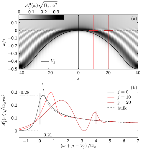
Figure 1: (a) Local Density of States $\mathcal{A}_{j}(\omega)$ (color scale) for the noninteracting, $U_{j}=0$, Hamiltonian Eq. (40) with potential (42) at $V_{g}\!=\!0$ (thick black line). (b) Local Density of States $\mathcal{A}_{j}(\omega)$ as a function of $(\omega-V_{j})/\Omega_{x}$ for a homogenous tight binding chain ($V_{j}=0$, grey line) and for the potential (42) at fixed site $j=0$ (blue), $j=10$ (green) and $j=20$ (red), indicated in (a) by vertical lines with corresponding colors.

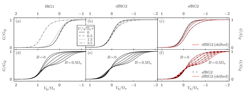
Figure 2: (a) to (c) Conductance $G$, as a function of gate-voltage, $V_{g}$, at zero magnetic field, $B\!=\!0$, for different values of interaction $U$. (d) to (f) Conductance $G$ at fixed interaction strength $U=3.5\sqrt{\Omega_{x}}$, for six equidistant magnetic fields $B$, between $0$ and $0.5\Omega_{x}$. Conductance is calculated using fRG1 (a, d), dfRG2 (b, c) or sfRG2 black lines in (c, f). Red lines in (c, f) show dfRG2 data repeated from (b, e) with a $U$-dependent shift, $\Delta V_{g}$, in $V_{g}$-direction ($\Delta V_{g}=0$, $0.001$, $0.02$ and $0.15\Omega_{x}$ for $U=0$, $0.5$, $1,5$ and $3.5\sqrt{\Omega_{x}\tau}$ respectively)

IV.3 Conductance of a QPC

Having discussed the properties of the noninteracting model, we continue with the fRG-results at finite interaction. For this we first define the spatial dependence of the interaction $U_{j}$, which, for the one-dimensional model is an effective one-dimensional interaction resulting from integrating out two space dimensions. Its strength depends on the geometry, and is larger if the spatial confinement perpendicular to the one-dimensional system is smaller. We assume that this confinement is independent of the position in the transport direction in the center of the QPC, with $U_{j=0}\!=\!U$. This is a fair assumption for a saddle point approximation of the two-dimensional QPC potential. For $|j|\to N^{\prime}=\frac{N-1}{2}$, $U_{j}$ drops smoothly to zero, describing the adiabatic coupling to the two-dimensional electron system, represented by the semi-infinite tight binding chain.

In Ref. Bauer et al., 2013 we showed that the 0.7-anomaly is caused by the van Hove ridge in the LDOS discussed above. Its apex crosses the chemical potential when the QPC is tuned into the sub-open regime, i.e. the regime where the conductance takes values $0.5G_{Q}<G<0.9G_{Q}$. This high LDOS at the chemical potential enhances effect of interactions by two main mechanisms: first, the effective Hartree barrier depends nonlinearly on gate-voltage and magnetic field, causing an enhanced elastic backscattering; and second, due to the high LDOS inelastic backscattering is enhanced once a phase space is opened up by a finite temperature or source-drain voltage. Both effects reduce the conductance in the sub-open regime, causing the 0.7-anomaly. Since interactions are enhanced by the LDOS, the relevant dimensionless interaction strength is $U_{j}\mathcal{A}_{j}(\mu)a$, which scales like $U/\sqrt{\Omega_{x}\tau}$ in the sub-open regime.

In this paper we will concentrate on examining how the reliability of the method depends on the interaction, without explaining the physical mechanism underlying the 0.7-anomaly in detail (for the latter we refer to Ref. Bauer et al., 2013). For the model Eq. (40) no reliable results are availible from other methods to which we could have compared our own. Instead, we here compare the results of the different fRG-schemes fRG1, sfRG2 and dfRG2. These schemes differ in the prefactor of the perturbative expansion of terms in order $U^{2}$ and higher. If these terms are important the three approximation schemes will deviate from each other. Hence, the qualitative and quantitative reliability can be deduced from the qualitative and quantitative deviations between these schemes.

The first observable we discuss is the linear response conductance at zero teperatureDatta (1997):

$$G=\frac{e^{2}}{h}\sum_{\sigma}\left|2\pi\rho^{\sigma}(i0^{+})\mathcal{G}_{-N^{\prime}N^{\prime}}^{\sigma}(i0^{+})\right|^{2}\,,$$ (45)

where $\rho(\omega)$ is the density of states at the boundary of a semi-infinite tight-binding chain, representing the two-dimensional leads (for a derivation of the boundary Green’s function, see appendix Sec. A).

Particularly interesting in studying the 0.7-anomaly in QPCs is the shape of the conductance trace as a function of applied gate voltage in the region where its value (in units of $G_{Q}$) changes from zero to one, and how this shape changes with external parameters, such as applied magnetic field. First of all, we emphasize the good qualitative agreement of all three approximation schemes with each other as well as with experimental results, compare Figs. 2 (d), (e) and (f) with Ref. Thomas et al., 1996; Cronenwett et al., 2002 (A direct comparison of dfRG2 with experiment is given in Ref. Bauer et al., 2013). This confirms that the method qualitatively captures the physical mechanism with respect to the conductance at zero temperature very well.

For a more quantitative analysis we first consider the position of the conductance step, say $V_{\rm po}$; even though the actual position of the step is of minor interest experimentally, it gives information about how accurate Hartree-type correlations are treated. Figs. 2 (a), (b), and (c) show the conductance at $B=0$ for increasing values of interaction $U$ for fRG1, dfRG2, and sfRG2 respectively. While for dfRG2 and for sfRG2 $V_{\rm po}$ decreases with interaction, its behavior for fRG1 is non-monotonic: $V_{\rm po}$ decreases slightly at small values of interaction, and increases strongly at larger values of interaction. Hence the conductance at large interaction is higher than the bare, $U=0$, value. This behavior is unphysical: whenever the density is nonzero, an increase in $U$ should cause an increase in the effective barrier height due to coulomb repulsion, and hence a decrease in the conductance. This artifact is significantly reduced by the vertex-flow of both dfRG2 and sfRG2. For the latter, interactions suppress the conductance more strongly than for the former. Due to these deviations between the three schemes, we cannot make a quantitative statement about the exact position of the conductance step $V_{\rm po}$.

The deviations just discussed make quantitative comparisons between these methods (or with others, such as RPA) difficult if interactions are large. The reason for the difficulty is that the $V_{g}$-position of the conductance step depends sensitively on the precise way in which Hartree-type correlations are treated and hence differ for each of the above schemes. Hence it would not be meaningful to compare their predictions for physical quantities calculated at a given value of $V_{g}$; instead, it is only meaningful to compare the shape of their evolution with $V_{g}$. Actually, the same is true for physical quantities that are dominated by Fock-type correlations, since internal propagators have to be dressed by Hartree diagrams. Doing this is crucial for inhomogeneous systems such as ours, since an inhomogeneous density causes these Hartree contributions to have a significant dependence on position and gate voltage. In the fRG approach the feedback of the self-energy Eq. (9) always guarantees that internal lines are dressed in a self-consistent way.

Let us now compare the shapes of the $V_{g}$-dependent conductance curves for dfRG2 and sfRG2. To this end, replotted the dfRG2 data from Fig. 2 (b) in Fig. 2 (c), with a $U$-dependent shift $\Delta V_{g}$ in $V_{g}$-direction (red lines). It can be seen from comparison with sfRG2 data, that the shapes of the conductance curves are almost identical.

Next we analyze the shape of the conductance step at finite interaction, and how it develops with magnetic field. The effect of an increasing magnetic field is qualitatively similar for the three approximation schemes [see Figs. 2 (d), (e) and (f)]: the conductance step develops into a spin resolved double step, in an asymmetric way: while the curves hardly change for $V_{g}$ values where $G<0.5G_{Q}$, they are strongly suppressed in the sub-open regime, where the LDOS is large. For fRG1 the $V_{g}$-range where the lowest magnetic field, $B=0.1\Omega_{x}$, significantly reduces the conductance w.r.t. the conductance at $B\!=\!0$, is larger than for dfRG2 and sfRG2. This is related to the fact, that the magnetoconductance, the change of conductance with magnetic field, within fRG1 is negative even for $V_{g}$ values where conductance is close to zero [this effect is too small to be visible in Fig. 2 (d)]. Since this is not the case for dfRG2 and sfRG2 it is not possible to make a reliable statement about the sign of the magnetoconductance in the tunnel regime. Again we reproduced the dfRG2 data from Fig. 2 (e) in Fig. 2 (f) with a shift $\Delta V_{g}$ in $V_{g}$ (red line) in order to compare their shape with the sfRG2 data (black dashed line). The effect of the magnetic field on the conductance within sfRG is slightly larger for small fields and slightly smaller for large fields, than for the dfRG2 results. Based on the facts, that, first, the deviations between dfRG2 and sfRG2 are small and, second, sfRG2 is computationally much cheaper than dfRG2, we conclude that for preliminary studies, or when scanning a large parameter space, one should favor sfRG2 whenever it is sufficient to know the static part of vertex functions.

IV.4 Susceptiblity

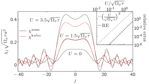
Figure 3: Local spin-susceptibility $\chi_{j}$, Eq. (31),as a function of site index, for the QPC potential Eq. (42), at $V_{g}\!=\!-\Omega_{x}/4$, calculated using dfRG2 via the the numerical derivative of the local magnetisation, $\chi^{\rm num}$ (black lines), as well as via the Kubo formula (35), $\chi^{\rm kubo}$ (red lines), for three different values of interaction. Inset: relative error ${\rm RE}$ (46) (dots), as a function of interaction $U$, on a log-log scale. The error scales as $U^{3}$ (compare dashed line), since dfRG2 is exact to second order in the interaction $U$.

As explained in reference Bauer et al., 2013, the 0.7-anomaly is related to an enhanced spin susceptibility in the sub-open regime of the QPC. For this quantity an estimate of the error is available within the dfRG2 approximation scheme. We note that the spin-susceptibility defined in equation (31) can be calculated in two ways: by numerical differentiation of the magnetization for a small magnetic field, $\chi^{\rm num}$, or via equation (35), $\chi^{\rm kubo}$. Like the conductance, the value of $\chi$ is not known exactly. Thus we argue here as in the previous section. $\chi^{\rm num}$ and $\chi^{\rm kubo}$ are both exact to second order in the interaction, as can easily be checked, but they differ in terms that are of order $U^{3}$ and higher. If the difference of $\chi^{\rm num}$ and $\chi^{\rm kubo}$ is significant, the higher order terms are non-negligible, and the results cannot be trusted.

In reference Bauer et al., 2013 we showed that $\chi^{\rm num}_{j}$ is enhanced due to the inhomogeneity of the QPC potential and in addition amplified by interactions. It has a strong $V_{g}$-dependence, and is maximal when the QPC is tuned into the sub-open regime. In this regime, at $V_{g}=-\Omega_{x}/4$, we compare $\chi^{\rm num}$ (Fig. 3 black lines) with $\chi^{\rm kubo}$ (Fig. 3 red lines) for different values of interaction. For intermediate values of interaction $U=1.5\sqrt{\Omega_{x}\tau}$ both results are essentially identical, while for a larger value of interaction $U=3.5\sqrt{\Omega_{x}\tau}$ deviations are clearly visible, however still not too large. The qualitative features that the susceptibility strongly increases with interaction, and that it is enhanced in the center of the QPC, emphasized in Ref. Bauer et al., 2013, are confirmed by both results. Furthermore they coincide in their spatial structure, i.e. two maxima in the center and a decaying oscillating behavior. This spatial structure is mainly given by the LDOS at the chemical potential (see Sec.  IV.2) and enhanced by interactions.

For a better quantification we define the relative error:

$${\rm RE}=2\frac{\sum_{j}\left|\chi_{j}^{\rm kubo}-\chi_{j}^{\rm num}\right|}{\sum_{j}\left|\chi_{j}^{\rm kubo}+\chi_{j}^{\rm num}\right|}\,.$$ (46)

This error is shown on a log-log scale in the inset of Fig. 3 (dots). The relative error scales like $U^{3}$, since dfRG2, and thus $\chi^{\rm num}$ and $\chi^{\rm kubo}$ are exact to second order in $U$. For the larger value of interaction, $U=3.5\sqrt{\tau\Omega_{x}}$, the relative error of about $18\%$ is quite significant and thus the value of $\chi$ is quantitatively not reliable. The reason for this is that the dimensionless interaction strength $U_{j}\mathcal{A}_{j}(\mu)a\approx 3.5\cdot 0.3\approx 1$ is already close to one. Nevertheless the error is still dominated by the third order term, implying that it is controlled.

Finally we note that the spin-susceptibility in the RPA approximation

$$\chi_{i}^{\rm RPA}=\sum_{j}\left[{W}^{d}(0)\left[1+\mathcal{U}{W}^{d}(0)\right]^{-1}\right]_{ij}\;.$$ (47)

diverges at an interaction strength for which fRG is still well-behaved. For example, if bare internal propagators are used to calculate ${W}^{d}$, $\chi_{i}^{\rm RPA}(V_{g})$ turns out to diverge at $U\simeq 3.3\sqrt{\Omega_{x}\tau}$. Moreover, the value of $\chi^{\rm RPA}$ and thus also the $U$-value for which it diverges depends on how one chooses to treat interactions for internal propagators of ${W}^{d}$. However RPA itself gives no recipe how to do this. In contrast, the fRG approach gives a systematic framework for computing the two-particle vertex, the self-energy, and their feedback into each other, in a way that moderates competing instabilities in an unbiased way (as mentioned in section III).

V Conclusion and Outlook

We have derived a fRG based approximation scheme, called the coupled-ladder approximation (CLA), for spin-full fermionic tight binding models with a local interaction and an arbitrary potential. The main applications are systems with a significant spatial dependence, in particular, models where the electron density significantly changes with the position in real space.

The CLA is formulated within the context of third-order-truncated fRG schemes, in which the three particle vertex is set to zero, while the flow of the two particle vertex is fully incorporated. The CLA retains two of the main properties of third-order-truncated fRG: it is exact to second order, and sums up diagrams of the RPA in all channels. Since the CLA is based on a perturbative argument, it is reliable only if interactions are not too large.

We analyzed in detail the reliability of this approach for a one-dimensional tight binding model with a parabolic potential barrier representing a QPC. For this we compared results for the conductance and the spin susceptibility calculated using different approaches within the fRG for different interactions up to $U\!=\!3.5\sqrt{\Omega_{x}\tau}$. We identified the magnetic field dependence of the conductance and the enhanced susceptibility related to the 0.7 anomaly,Bauer et al. (2013) as robust properties of the model.

Finally, let us comment briefly on the prospects of using the CLA approach presented here to obtain finite-temperature results. While the formulas for the local density $n$ and the local susceptibility $\chi$, Eq. (35), are valid for arbitrary temperature $T$, the conductance formula Eq. (45) holds only for the case of zero temperature. The generalization of this formula to finite temperatureOguri (2001) involves an analytic continuation to the real axis for both self-energy and vertex w.r.t. their frequency arguments. However, performing such an analytic continuation for numerical data is a mathematically ill-defined problem and turns out to be especially difficult for matrix-valued functions.

One possibility to avoid this complication is to formulate our CLA scheme on the Keldysh contour, in which case there are several different possibilities for introducing the fRG flow parameter Jakobs (2009). (For a fRG treatment of the Single Impurity Anderson Model see Ref. Jakobs et al., 2010a). When using Keldysh fRG to treat equilibrium properties, the number of independent correlators can be reduced by exploiting the Kubo-Martin-Schwinger conditions.Jakobs et al. (2010b) Moreover, Keldysh fRG in principle also allows non-equilibrium properties to be calculated. The actual implementation of Keldysh fRG for our model will be nontrivial, though, in particular since numerical integrations along the real axis, where Green’s functions can have poles, can be challenging. Another problem at finite temperature is the violation of particle conservation due to the fRG truncation (5),Enss (2005). The extent of this violation might be reduced by by implementing the modified vertex flow suggested by Katanin. Katanin (2004) We believe that it would be worth pursuing work in these directions.

Appendix A Projection method

The propagator in the fRG flow Eqs. (8) and (12), in general, lives on an infinite-dimensional chain. However, since the interacting region has finite extent, we only need to evaluate it on an $N$-dimensional subspace. Furthermore, for the evaluation of Eq. (35) we need to calculate the sum over all site indices $j$, including the infinite number of sites in the leads. To this end we perform a standard projection procedureKarrasch (2006); Taylor (1972). With this method the influence of the leads on the propagator and their contribution to the sum can be calculated analytically if the diagonalization of the leads is known analytically. Therefore we define projection operators $C$ and $L$, with $C^{2}=C$, $L^{2}=L$ and $L+C=\mathbb{1}$ which divide the Hilbert space into the part that describes the leads, $L$, and the finite dimensional part that describes the central region where interaction is non-zero, $C$. Furthermore, we define for a given quadratic Hamiltonian $H$ (for an interacting system $H$ is replaced by $H_{0}\!+\!\Sigma$), $H_{c}=CHC$, $H_{c}=CHC$, $H_{cl}=CHL$, $H_{lc}=LHC$, $\omega_{l}=\omega L$ and $\omega_{c}=\omega C$ and write the Hamiltonian in the basis defined by the projections:

$$H=\left(\begin{array}[]{ccc}H_{c}&H_{cl}\\ H_{lc}&H_{l}\end{array}\right).$$ (50)

Consequently the Greens function in the same basis reads

$$\mathcal{G} = \begin{pmatrix}\omega_{c}-H_{c}&-H_{cl}\\ -H_{lc}&\omega_{l}-H_{l}\end{pmatrix}^{-1}=\begin{pmatrix}\mathcal{G}_{c}&\mathcal{G}_{cl}\\ \mathcal{G}_{lc}&\mathcal{G}_{l}.\end{pmatrix}$$ (51)

with

$$\mathcal{G}_{c} =\frac{1}{\omega_{c}-H_{c}-H_{cl}g_{l}H_{lc}}\,, g_{l}=\frac{1}{\omega_{l}-H_{l}}\,,$$ (52a)

$$\mathcal{G}_{l} =\frac{1}{\omega_{l}-H_{l}-H_{lc}g_{c}H_{cl}}\,, g_{c}=\frac{1}{\omega_{c}-H_{c}}\,,$$ (52b)

$$\mathcal{G}_{cl} =\mathcal{G}_{c}H_{cl}g_{l}=g_{c}H_{cl}\mathcal{G}_{l}\,,$$ (52c)

$$\mathcal{G}_{lc} =g_{l}H_{lc}\mathcal{G}_{c}=\mathcal{G}_{l}H_{lc}g_{c}\,.$$ (52d)

In the following we will only use $\mathcal{G}_{l}$ and $g_{c}$ as well as $G_{cl}$ and $G_{lc}$ expressed in terms $\mathcal{G}_{l}$ and $g_{c}$, so we use the shorthands $\mathcal{G}=\mathcal{G}_{l}$ and $g=g_{l}$ (whether $\mathcal{G}$ lives on the infinite-dimensional Hilbert space, or on the subspace of the central contact, will be clear from its site indices).

For the case of the infinite tight-binding chain defined by Eq. (40), the central region extends from site $\!-\!N^{\prime}$ to site $N^{\prime}$, with $N^{\prime}=\frac{N-1}{2}$, and the coupling to the leads can be expressed as:

$$H_{cl} = -\tau\left(d^{\dagger}_{-N^{\prime}}d^{\leavevmode\nobreak\ }_{-N^{\prime}-1}+d^{\dagger}_{N^{\prime}}d^{\leavevmode\nobreak\ }_{N^{\prime}+1}\right)$$ (53a)

$$H_{lc} = H_{cl}^{\dagger}\;.$$ (53b)

Consequently

$$H_{cl}gH_{lc} = \tau^{2}\left(d^{\dagger}_{-N^{\prime}}d^{\leavevmode\nobreak\ }_{-N^{\prime}-1}+d^{\dagger}_{N^{\prime}}d^{\leavevmode\nobreak\ }_{N^{\prime}+1}\right)$$ (54)

$$\times g\left(d^{\dagger}_{-N^{\prime}-1}d^{\leavevmode\nobreak\ }_{-N^{\prime}}+d^{\dagger}_{N^{\prime}+1}d^{\leavevmode\nobreak\ }_{N^{\prime}}\right)$$

$$= \tau^{2}b\left(n_{-N^{\prime}}+n_{N^{\prime}}\right),$$

where $b\!=\!g_{N^{\prime}+1,N^{\prime}+1}$ is the boundary Greens function of a half-infinite tight binding chain. Transforming into $k$-space and using the boundary condition $\langle d^{\dagger}_{N^{\prime}}d_{k}\rangle=0$ we get $\langle d^{\dagger}_{N^{\prime}+1}d_{k}\rangle\propto\sin^{2}(k)$. Together with the dispersion $\varepsilon_{k}=-\mu-2\tau\cos(k)$ and the proper normalisation, this yields for ${\rm Im}(\omega_{n})>0$:

$$b(\omega_{n}) = \frac{1}{\pi}\int_{-\pi}^{\pi}dk\frac{\sin^{2}(k)}{\omega_{n}+\mu+2\tau\cos(k)}$$ (55)

$$= \frac{1}{2\tau^{2}}\left[\omega_{n}\!+\!\mu-i\leavevmode\nobreak\ \sqrt{4\tau^{2}-(\omega_{n}+\mu)^{2}}\right].\qquad$$

The square root is defined to have a positive real part, and $b(-\omega_{n})=b^{*}(\omega_{n})$. (For the spin-dependent boundary Green’s function at finite magnetic field, $\mu$ has to be replaced by $\mu+\sigma B/2$).

Next we calculate the infinite sum in Eq. (35). We split the sum into three parts and take $k$ and $l$ to be site indices in the central region.

$$\sum_{j=-\infty}^{\infty}\mathcal{G}_{kj}\mathcal{G}_{jl}=\left(\sum_{j=-\infty}^{-N^{\prime}-1}+\sum_{j=-N^{\prime}}^{N^{\prime}}+\sum_{j=N^{\prime}+1}^{\infty}\right)\mathcal{G}_{jk}\mathcal{G}_{jl}=$$

$$=\sum_{j=-N^{\prime}}^{N^{\prime}}\mathcal{G}_{jk}\mathcal{G}_{jl}+\tau^{2}\mathcal{G}_{k,-N^{\prime}}h^{L}\mathcal{G}_{-N^{\prime},l}+\tau^{2}\mathcal{G}_{k,N^{\prime}}h^{R}\mathcal{G}_{N^{\prime},l},$$ (56)

with

$$h^{L} =\sum_{j=-\infty}^{-N^{\prime}-1}g_{-\!N^{\prime}\!-\!1,j}g_{j,\!-\!N^{\prime}\!-\!1},$$ (57a)

$$h^{R} =\sum_{j=N^{\prime}+1}^{\infty}g_{N^{\prime}+1,j}g_{j,N^{\prime}+1},$$ (57b)

where we made use of Eqs. (52c), (52d) and (53).

Finally we note that the last two terms are identical and given by

$$h(\omega_{n})\! \!=\! \!h^{L}(\omega_{n})=h^{R}(\omega_{n})=\left[g^{2}(i\omega_{n})\right]_{N^{\prime}+1,N^{\prime}+1}=$$ (58)

$$\!=\! \!\frac{1}{\pi}\int_{-\pi}^{\pi}dk\frac{\sin(k)^{2}}{\left(\omega_{n}+\mu+2\tau\cos(k)\right)^{2}}=$$

$$\!=\! \!\frac{1}{2\tau^{2}}\!\left(\frac{\omega_{n}+\mu}{\omega_{n}+\mu-2\tau}\sqrt{\frac{\omega_{n}+\mu-2\tau}{\omega_{n}+\mu+2\tau}}-1\right)\!.\;\;\qquad$$

References

- Bauer et al. (2013) F. Bauer, J. Heyder, E. Schubert, D. Borowsky, D. Taubert, B. Bruognolo, D. Schuh, W. Wegscheider, J. von Delft, and S. Ludwig, Nature 501, 73 (2013).
- Wetterich (1993) C. Wetterich, Physics Letters B 301, 90 (1993).
- Metzner et al. (2012) W. Metzner, M. Salmhofer, C. Honerkamp, V. Meden, and K. Schönhammer, Rev. Mod. Phys. 84, 299 (2012).
- Meden et al. (2002) V. Meden, W. Metzner, U. Schollwöck, and K. Schönhammer, Phys. Rev. B 65, 045318 (2002).
- Andergassen et al. (2004) S. Andergassen, T. Enss, V. Meden, W. Metzner, U. Schollwöck, and K. Schönhammer, Phys. Rev. B 70, 075102 (2004).
- Andergassen et al. (2006) S. Andergassen, T. Enss, V. Meden, W. Metzner, U. Schollwöck, and K. Schönhammer, Physical Review B 73, 045125 (2006).
- Karrasch et al. (2008) C. Karrasch, R. Hedden, R. Peters, T. Pruschke, K. Schönhammer, and V. Meden, Journal of Physics: Condensed Matter 20, 345205 (2008).
- Karrasch (2006) C. Karrasch, Transport Through Correlated Quantum Dots – A Functional Renormalization Group Approach, Master’s thesis, Georg-August Universität Göttingen (2006), arXiv:cond-mat/0612329v1.
- Husemann et al. (2012) C. Husemann, K.-U. Giering, and M. Salmhofer, Phys. Rev. B 85, 075121 (2012).
- Giering and Salmhofer (2012) K.-U. Giering and M. Salmhofer, Phys. Rev. B 86, 245122 (2012).
- Jakobs et al. (2010a) S. G. Jakobs, M. Pletyukhov, and H. Schoeller, Phys. Rev. B 81, 195109 (2010a).
- Honerkamp (2001) C. Honerkamp, European Physical Journal B 21, 81 (2001).
- Honerkamp and Salmhofer (2003) C. Honerkamp and M. Salmhofer, Phys. Rev. B 67, 174504 (2003).
- van Wees et al. (1988) B. J. van Wees, H. van Houten, C. W. J. Beenakker, J. G. Williamson, L. P. Kouwenhoven, D. van der Marel, and C. T. Foxon, Phys. Rev. Lett. 60, 848 (1988).
- Wharam et al. (1988) D. A. Wharam, T. J. Thornton, R. Newbury, M. Pepper, H. Ahmed, J. E. F. Frost, D. G. Hasko, D. C. Peacock, D. A. Ritchie, and G. A. C. Jones, Journal of Physics C: Solid State Physics 21, L209 (1988).
- Büttiker (1990) M. Büttiker, Phys. Rev. B 41, 7906 (1990).
- Thomas et al. (1996) K. J. Thomas, J. T. Nicholls, M. Y. Simmons, M. Pepper, D. R. Mace, and D. A. Ritchie, Phys. Rev. Lett. 77, 135 (1996).
- Appleyard et al. (2000) N. J. Appleyard, J. T. Nicholls, M. Pepper, W. R. Tribe, M. Y. Simmons, and D. A. Ritchie, Phys. Rev. B 62, R16275 (2000).
- Cronenwett et al. (2002) S. M. Cronenwett, H. J. Lynch, D. Goldhaber-Gordon, L. P. Kouwenhoven, C. M. Marcus, K. Hirose, N. S. Wingreen, and V. Umansky, Phys. Rev. Lett. 88, 226805 (2002).
- Taylor (1972) J. Taylor, Scattering theory: the quantum theory on nonrelativistic collisions (Wiley, 1972).
- Morris (1994) T. R. Morris, International Journal of Modern Physics A 09, 2411 (1994).
- Jakobs et al. (2007) S. G. Jakobs, V. Meden, and H. Schoeller, Phys. Rev. Lett. 99, 150603 (2007).
- Bauer (2008) F. Bauer, 0.7 Anomaly of Quantum Point Contacts: Treatment of Interactions with Functional Renormalization Group., Master’s thesis, LMU-München (2008).
- Dormand and Prince (1980) J. Dormand and P. Prince, Journal of Computational and Applied Mathematics 6, 19 (1980).
- Schuricht et al. (2013) D. Schuricht, S. Andergassen, and V. Meden, Journal of Physics: Condensed Matter 25, 014003 (2013).
- Forsythe and Wasow (1960) G. Forsythe and W. Wasow, Finite-difference methods for partial differential equations, Applied mathematics series (Wiley, 1960).
- Datta (1997) S. Datta, Electronic Transport in Mesoscopic Systems, Cambridge Studies in Semiconductor Physics and Microelectronic Engineering (Cambridge University Press, 1997).
- Oguri (2001) A. Oguri, Journal of the Physical Society of Japan 70, 2666 (2001).
- Jakobs (2009) S. G. Jakobs, Functional renormalization group studies of quantum transport through mesoscopic systems, Ph.D. thesis, RWTH Aachen (2009).
- Jakobs et al. (2010b) S. G. Jakobs, M. Pletyukhov, and H. Schoeller, Journal of Physics A: Mathematical and Theoretical 43, 103001 (2010b).
- Enss (2005) T. Enss, Renormalization, Conservation Laws and Transport in Correlated Electron Systems, Ph.D. thesis, University of Stuttgart (2005), arXiv:cond-mat/0504703v1.
- Katanin (2004) A. A. Katanin, Phys. Rev. B 70, 115109 (2004).