A Fractal and Scale-free Model of Complex Networks with Hub Attraction Behaviors

Abstract

It is widely believed that fractality of complex networks origins from hub repulsion behaviors (anticorrelation or disassortativity), which means large degree nodes tend to connect with small degree nodes. This hypothesis was demonstrated by a dynamical growth model, which evolves as the inverse renormalization procedure proposed by Song et al. Now we find that the dynamical growth model is based on the assumption that all the cross-boxes links has the same probability $e$ to link to the most connected nodes inside each box. Therefore, we modify the growth model by adopting the flexible probability $e$, which makes hubs have higher probability to connect with hubs than non-hubs. With this model, we find some fractal and scale-free networks have hub attraction behaviors (correlation or assortativity). The results are the counter-examples of former beliefs.

Citation

1 Introduction

Fractal Geometry theory is proposed by Mandelbrot to explain the mathematical set which has a fractal dimension exceeds its topological dimension[1,2]. Fractals are patterns that exhibit self-similar at different length scales. Nowadays, more and more researchers focus on the study of complex networks. A critical property of complex networks is the degrees of nodes follow power law distribution[3,4,5]. The probability P(k) of number of connections $k$ to a node fulfill power-law relation:

$$P(k)\approx{k}^{-\gamma}.$$ (1)

As fractal geometry focus on mathematical set on Euclid space, some researchers wondered whether complex networks in topological space have fractality property [9,10]. Among them, Song et al’s researches of fractality property in complex networks have attracted extensive attentions. They proposed a renormalization procedure implemented by box covering method[6], which was inspired from ‘box counting’ method applied in Euclid space, to tile the networks into boxes with a given box size as shown in Fig.1. The box size ${\ell}_{B}$ is the upper bound of shortest path between nodes in each box. The process is iterated until only single node left. Through the procedure, they found that many real world networks, such as the World Wide Web, Protein-Protein Interaction networks, and Cellular networks have scale-invariance and fractality properties. The scale-invariance means the degree distribution of renormalized networks still follow the power law under different length scale renormalizations, and the fractality means the number of boxes ${N}_{B}$, which is needed to cover the whole network, is approximate to power $-{d}_{B}$ of the box size ${\ell}_{B}$. This can be defined as equation(2):

$${N}_{B}({\ell}_{B})\approx{{\ell}_{B}}^{-{d}_{B}}.$$ (2)

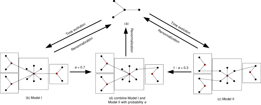
Figure 1: Network dynamical growth with parameters: degree multiplier m = 2 and box size ${\ell}_{B}=3$. The dynamical growth process can be seen as the inverse renormalization procedure. (a), Four nodes at t = 0 that could growth to networks in (b), (c) and (d) through time evolution. (b), Mode I alone, where most connected nodes in each box connect directly to each other. (c), Mode II alone, where boxes connected by less connected node. (d), Combination of Mode I and II with probability e = 0.7.

Song et al analyzed the origin of the fractality of complex networks later[7]. They proposed the dynamical growth model (DMG) from the perspective of networks evolution based on the ideas of Barabási-Albert model[4]. It is the inverse renormalization procedure as showed in Fig.1. The network evolves as time step t increases. Every node at time step $t-1$ with degree $k(t-1)$ will evolve to a visual box with $mk(t-1)$ new nodes (black nodes) generated inside each box. And initial nodes (red nodes) connect to all the new nodes in each box. They proposed two kinds of models with difference on generating cross-boxes links. In Model I, most connected nodes in each box connect directly to each other as shown in Fig.1(b), while in Model II, links between boxes connect to less connected nodes inside each boxes as shown in Fig.1(c). The extensive growth model is the combination of Model I and Model II with a stationary probability e through whole network as showed in Fig.1(d), where e is defined as the measurement of the level of ‘hub’ attraction. Their results have shown networks with higher probability of e tend to be non-fractal, yet networks with lower probability of e inclined to be fractal. Therefore, they concluded that ‘hub’ repulsion is the cause of fractality.

Similar research found that fractal scale-free networks are disassortative mixing[14]. There was also research work illustrated the fractal networks have to fulfill the criticality condition: the skeleton, which has branching tree structure, grows from root node (most connected node in network) perpetually with offspring neither flourishing nor dying out[16].

However, the above assertions are based on experiments rather than theoretical proof. In this paper, we get different results by simply modifying the DGM model. As we know, hubs are defined as the most connected nodes in the whole network[3]. We notice Song et al presumed the most connected nodes in each box as the hubs of whole network. In fact, due to the power law degree distribution, most of the highest degree nodes in boxes have much lower degree compared with the real hubs in the network. Therefore, we apply flexible probability $e$ mechanism to make real hubs have higher probability to connect with each other, while lower the probability of connection between non-hub nodes. By applying this mechanism, we can achieve fractal and scale-free networks (HADGM) with strong hub attraction. Moreover, we find relative researches that supports our statement. Some optimization networks exhibit both fractality and assortativity mixing properties[18]. Our research gives a fundamental challenge to the former researches on the origin of the fractal complex networks. We notice the fractality has strong correlation with the diameter of networks. As long as the diameter grows exponential with time evolution, the networks will preserve fractality property.

This paper is organized as follows. In Sec.2, we introduce the HAGMD model. The subsections present the flexible probability $e$ mechanism and inside box link-growth method. In Sec.3, we analyze the properties of HAGMD model, such as fractality, scale-free and correlations. In Sec.4, we introduce the fractal optimization network and compare the assortativity of all the models. At last, In Sec.5, we summery our works and discuss the origin of fractality.

2 Hub attraction dynamical growth model

As shown in Fig.2, based on the dynamical growth framework of DGM model, we make probability $e$ flexible (hubs have higher probability to connect to each other). This mechanism alone could make hubs connected together, while persevering the fractality property. However, we find DGM networks are only spinning trees without loops, which are not similar with real networks. Therefore, we also propose the inside box link-growth method, which add the correlation between high degree nodes.

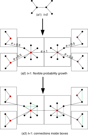
Figure 2: Hub attraction dynamical growth model. (a1), Five nodes at time step $t=0$. (a2) Dynamical growth network at $t=1$ with flexible probability $e$, which $e=1$ between high degree nodes, and $e=0.5$ between low degree nodes. (a3) The method of generating connections inside box (green line), where we random pick one new generated nodes and link it to other $\tilde{k}(t-1)$ new nodes. (b) HADGM network at time step $t=2$ which have initial 5 nodes at $t=0$ .

2.1 Flexible probability e mechanism

In the dynamical growth processes, each edge at time step $t-1$ will become cross-boxes link at time step $t$. We define probability e as piecewise function depending on the degrees of nodes (${k}_{1}(t-1)$ and ${k}_{2}(t-1)$) attached on both side of edge at time step $t-1$. As shown in equation(3):

$$e({k}_{1}(t-1),{k}_{2}(t-1))=\begin{cases}a&\text{ if }\frac{{k}_{1}(t-1)}{{k}_{max}(t-1)}>T\>\text{ and }\>\frac{{k}_{2}(t-1)}{{k}_{max}(t-1)}>T\\ b&\text{ if }\frac{{k}_{1}(t-1)}{{k}_{max}(t-1)}\leqslant T\>\>\>\text{ or}\>\>\>\>\frac{{k}_{2}(t-1)}{{k}_{max}(t-1)}\leqslant T\end{cases}\\ .$$ (3)

where $T,a,b$ are predefined parameters with domain as $0\leqslant b<a\leqslant 1$ , $0<T\leqslant 1$, and ${k}_{max}(t-1)$ is the max degree in network at time step $t-1$. Therefore, hubs in the network have higher probability to connect to each other, we can even define $a=1$ to let all hubs connected with each other as shown in Fig.2(a2) and Fig.2(b), where $T=0.5$ and $b=0.5$.

2.2 Inside box link-growth method

As shown in Fig.2(a3), in each time step of dynamical growth, we apply inside box link-growth method after the nodes growth phase. In time step $t$, we add $\tilde{k}(t-1)$ links in each box. Therefore, we add $2\tilde{K}(t-1)$ links in the whole network, where $\tilde{K}(t)$ is the total number of links at time t. The method does not affect the fractality and scale-free properties of the networks, but it increase the level of correlation of the networks. We will prove them in the following paragraph.

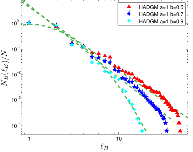
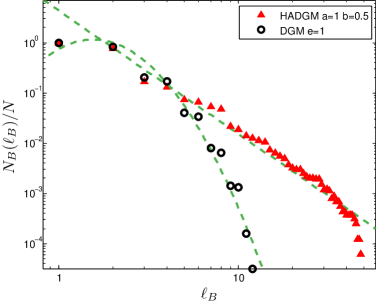
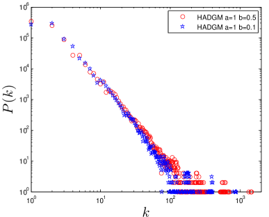
Figure 3: (a), Log-Log plot of ${N}_{B}({\ell}_{B})$ vs ${\ell}_{B}$ of HADGM networks with difference on parameter $b$. HADGM networks shows fractal property with $b=0.5$ and $b=0.7$, as $b$ increase to $0.9$ the network becomes non-fractal. (b), Comparison of ${N}_{B}({\ell}_{B})$ vs ${\ell}_{B}$ of HADGM network (fractal with $a=1$, $b=0.5$) and DGM network (non-fractal with $e=1$). (c), Degree distribution of HADGM networks with same parameters $a=1$, $T=0.5$ and $m=2$, while have difference on $b=0.5$ (red circle) and $b=0.1$ (blue star).

3 Properties of HADGM

In order to measure the properties of HADGM networks, we apply mathematic framework as equation(4) (Further deduction see the Appendix).

$$\begin{split}\tilde{N}(t)&\approx(2m+3)\tilde{N}(t-1)\;\;for\;\;t>1,\\ \tilde{k}(t)&=(m+\bar{e})\tilde{k}(t-1),\\ \tilde{L}(t)&=(3-2\bar{e})\tilde{L}(t-1)+2e,\end{split}$$ (4)

where $\tilde{N}(t)$ is the total number of nodes at time step $t$, $\tilde{k}(t)$ is the maximum degree inside a box at time step $t$, $\tilde{L}(t)$ is the diameter of the network at time step $t$, and $\bar{e}$ is the average of flexible probability $e$.

3.0.1 Fractality of HADGM

The networks evolve dynamically as the inverse renormalization procedure. Each node at time step $t-1$ will grow into a virtual box at time step $t$, thus based on equation(4) we have $\tilde{N}({t}_{1})/\tilde{N}({t}_{2})={N}_{B}({\ell}_{B})/N=(2m+3)^{{t}_{1}-{t}_{2}}$. And we also have $(\tilde{L}({t}_{2})+{L}_{0})/(\tilde{L}({t}_{1})+{L}_{0})={\ell}_{B}+{L}_{0}=(3-2\bar{e})^{{t}_{2}-{t}_{1}}$, where ${L}_{0}$ is the initial diameter[7]. Therefore, by inputting equation(2) and replacing the time interval ${{t}_{2}-{t}_{1}}$, we have fractal dimension ${d}_{B}$ as:

$${d}_{B}=\ln(2m+3)/\ln(3-2\bar{e}).$$ (5)

Due to the power law degree distribution, for $T\geqslant 0.5$ the average of probability $\bar{e}$ is close to value $b$. Thus, if we choose low value of $b$, the average probability $\bar{e}$ is obviously lower than $1$. So we will have finite fractal dimension ${d}_{B}$, which imply the fractality of HADGM. As shown in Fig.3(a), we apply box covering algorithm[8,11] to HADGM networks, which have different value $b$ and other parameters are the same. Thus, we find the HADGM networks are fractal if $b<0.9$. We notice when $b$ increase to a certain point $b=0.9$, then $\bar{e}\rightarrow 1$ and ${d}_{B}\rightarrow\infty$, so the HADGM network become non-fractal.

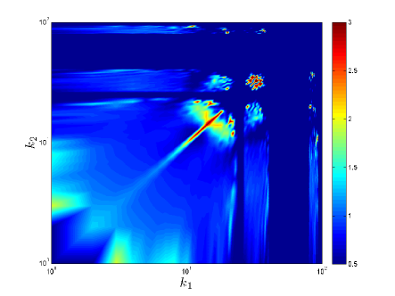
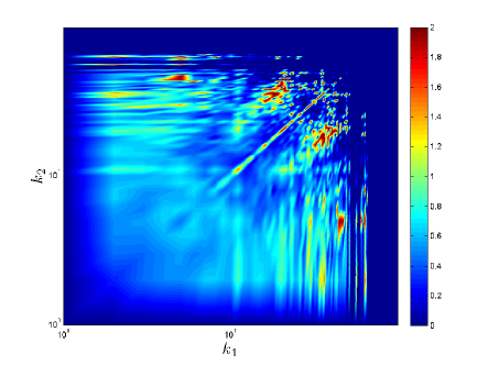
Figure 4: Comparison of Correlation : Different colors relate to different strength of correlation. Red color in the plot represent strong correlation. HADGM network shows stronger correlation between high degree nodes than other two networks. (a) Plot of ${R}_{HADGM}({k}_{1},{k}_{2})/{R}_{DGM}({k}_{1},{k}_{2})$ that compared correlation of HADGM network (fractal with $a=1$, $b=0.5$) with DGM network (non-fractal with $e=1$) (b) Plot of ${R}_{HADGM}({k}_{1},{k}_{2})/{R}_{WWW}({k}_{1},{k}_{2})$ that compared correlation of HADGM network (fractal with $a=1$, $b=0.5$) with the World Wide Web

3.0.2 Scale-free of HADGM

The recursive growth of $\tilde{k}(t)$ lead to the power law degree distribution of HADGM networks as shown in equation(4). The results are illustrated in Fig.3(c), the HADGM networks with different parameter $b$ show clear power law degree distribution with fat tail. And the two HADGM networks have differences on slope of the power law curve due to the difference on average probability $\bar{e}$.

3.0.3 Correlation and Fractality

Former research[7] asserted that fractal networks tend to show anticorrelation behaviors, while non-fractal networks exhibit correlation behaviors. The results are achieved by comparing the strength of anticorrelation between different networks. Such as non-fractal DGM model with $e=1$ has stronger correlation than fractal DGM model with $e=0.8$. However, our comparison results show the fractal HADGM model has even stronger correlation than non-fractal DGM model with $e=1$. Therefore, we get different results with the assertion that the hub repulsion behaviors give rise to fractality property.

The correlation is quantified by equation: $R({k}_{1},{k}_{2})=P({k}_{1},{k}_{2})/P_{r}({k}_{1},{k}_{2})$, which illustrates the correlation topological properties of a network[17]. Given a network $G$, the $P({k}_{1},{k}_{2})$ is defined as the joint probability of finding a node with degree ${k}_{1}$ linked to a node with degree ${k}_{2}$. $P_{r}({k}_{1},{k}_{2})$ is defined as joint probability of the null model ${G}^{{}^{\prime}}$ of the network $G$. The null model ${G}^{{}^{\prime}}$ is generated by randomly rewiring all links of $G$, while keeping the degree distribution. We compare the correlation feature of our fractal HADGM network ($a=1,b=0.5$) with non-fractal DGM network ($e=1$) and the World Wide Web (real-world network from Pajek Database[19]. The results are showed in Fig.4. The plots of ${R}_{HADGM}({k}_{1},{k}_{2})/{R}_{DGM}({k}_{1},{k}_{2})$ and ${R}_{HADGM}({k}_{1},{k}_{2})/{R}_{WWW}({k}_{1},{k}_{2})$ show fractal HADGM network ($a=1,b=0.5$) have stronger hub attraction behaviors than fractal the WWW network and non-fractal DGM network($e=1$).

4 Assortativity and Fractality

Relative research supports our statement is the optimization model proposed by Zheng et al, which can produce fractal scale-free network with hubs aggregation together[18]. This model has two optimization objectives: minimizing the summation of the degrees of the nodes and maximizing the summation of the degrees of the edges. And with constraint conditions that both the $\bar{\ell}$ (average shortest path) and xmin (minimum degree of nodes throughout the entire network) are set as non-negative constants. The edge degree between node i and node j is defined as: ${D}_{ij}={{k}_{i}}^{m}{{k}_{j}}^{n}$, where ${k}_{i}$ and ${k}_{j}$ are degree of node i and node j and m, n are non-negative constants. The optimization model can produce fractal scale-free network by stretching the parameter $\bar{\ell}$. Here, we choose fractal and scale-free network generated by optimization model for comparison with parameters: node number $N=1500$, $xmin=2$, $m=0$, $n=1$, $\bar{\ell}=40$.

Table 1: Fractality and Disassortativity

Network	N	r	Fractality	Disassortativity
DGM $e=1$	781245	-0.0347	NO	YES
HADGM $a=1,b=0.5$	784325	-0.0344	YES	YES for $k<100$
Optimization Network	1500	0.8354	YES	NO
The Internet	22963	-0.198	NO	YES

The assortativity can be measured by Pearson correlation coefficient $r$ [13], which can be rewrote as:

$$r=\frac{{M}^{-1}\sum_{i}{j}_{i}{k}_{i}-{\left[{M}^{-1}\sum_{i}\frac{1}{2}({j}_{i}+{k}_{i})\right]}^{2}}{{M}^{-1}\sum_{i}\frac{1}{2}({{j}_{i}}^{2}+{{k}_{i}}^{2})-{\left[{M}^{-1}\sum_{i}\frac{1}{2}{({j}_{i}+{k}_{i})}^{2}\right]}},$$ (6)

where ${j}_{i}$, ${k}_{i}$ are the degrees of the nodes at both sides of the $i$th edge, with $i=1,...,M$, and $M$ is the total number of edges in a network. The positive or negative of $r$ related to assortative or disassortative mixing. As shown in Table(1), the DGM network($e=1$) is non-fractal and disassortative, HADGM network ($a=1,b=0.5$) is fractal and disassortative, the optimization network is fractal and assortative, and real network the Internet of AS-level[20] is non-fractal and disassortative.

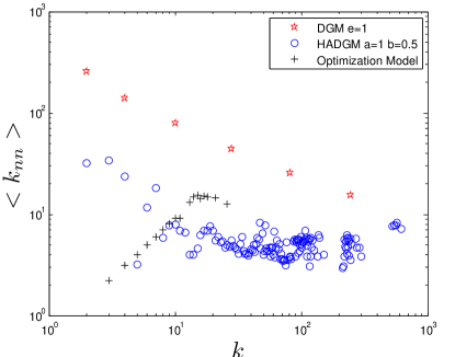
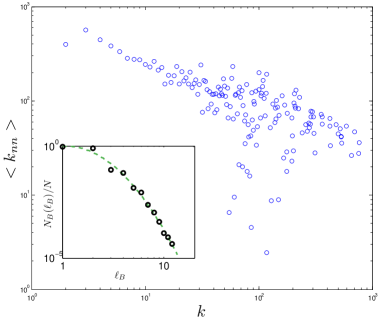
Figure 5: Neighbor connectivity of networks (a), Neighbor connectivity of the DGM network($e=1$)(red star), the HADGM network (blue circle) and the optimization fractal network (black cross) (b), Neighbor connectivity of the Internet. The inset shows the non-fractal of the Internet.

We also analyze the average degree of neighbors of a node with degree $k$ namely $<{k}_{nn}>$ of above networks. $<{k}_{nn}>$ is defined as $<{k}_{nn}>=\sum\limits_{{k}^{{}^{\prime}}}{k}^{{}^{\prime}}P({k}^{{}^{\prime}}|k)$, where $P({k}^{{}^{\prime}}|k)$ is the conditional probability of an edge of node with degree $k$ connect to a node with degree ${k}^{{}^{\prime}}$[12]. The network is assortative mixing if the slope of $k$ vs $<{k}_{nn}>$ curve is positive, which means high degree nodes tend to connect with high degree nodes, and is disassortative mixing if the slope of $k$ vs $<{k}_{nn}>$ curve is negative[13].

As Fig.5(a) showed, the fractal network produced by optimization model is assortative. And non-fractal DGM network($e=1$) is disassortative. It also shows the fractal HADGM network ($a=1,b=0.5$) is disassortative within low degrees range $k<100$, while assortative within high degrees range. The Internet shows obvious disassortative and non-fractal property as shown in Fig.5(b). Therefore, the results of the DGM network ($e=1$) , optimization model and the Internet are served as counter examples of the conjecture that self-similar scale-free networks are disassortative. Furthermore, the HADGM network ($a=1,b=0.5$) has stronger correlation than DMG network ($e=1$), yet the DMG network ($e=1$) is non-fractal and HADGM network ($a=1,b=0.5$) is fractal. Our results show the fractality property is independent of the assortative mixing feature.

5 Conclusion and Discussion

In this paper we proposed a new dynamical growth model, which can produce fractal networks with hub attraction behaviors. The model is designed by applying flexible probability of cross-boxes links mechanism and inside box link-growth method. More general models can also be proposed by applying different function of flexible probability $e$ or other kinds of inside link-growth mechanism.

Observing equations (4) and (5), the fractality property requires the diameter $\tilde{L}(t)$ of networks exponential growth through time evolution rather than linear growth. Therefore, we believe there is a structural equilibrium in fractal networks to keep the diameter $\tilde{L}(t)$ within a certain range. According to the topological structure of complex networks, we could divide a network into several layers as mentioned in[[15]. The most connected hub is consider as the center, other nodes are allocated in different layers depending on the distance to the center node. Hub attraction and booming growth in boundary are a pair of opposing force to maintain the structural equilibrium in fractal network. Hub attraction will lead to $\tilde{L}(t)$ to drop dramatically, while booming growth in boundary will result in $\tilde{L}(t)$ increasing sharply .

Appendix A Appendix

According to the HADGM model, at time step $t+1$ we generate $mk(t)$ new nodes for each node with degree $k(t)$ at time step $t$. Therefore, we have:

$$\tilde{N}(t+1)=\tilde{N}(t)+2m\tilde{K}(t),$$ (7)

where $\tilde{K}(t)$ is total number of links at time step $t$. At time step $t+1$, in the flexible probability growth phase we have $(2m+1)\tilde{K}(t)$ edges in network, then in the link-growth inside box phase we add $2\tilde{K}(t)$ edges. Thus, we have:

$$\tilde{K}(t+1)=(2m+3)\tilde{K}(t).$$ (8)

Combine equation(7) and equation(8), we have:

$$\tilde{N}(t)=\tilde{N}(0)+m\tilde{K}(0)\frac{(2m+3)^{t}-1}{m+1}.$$ (9)

Due to $\tilde{N}(t)\gg\tilde{N}(0)$, we can acquire $\tilde{N}(t)\thickapprox(2m+3)\tilde{N}(t-1)$ for $t>1$.

Considering the node degrees growth with time evolution, for Model I, alone we have $\tilde{k}(t)=(m+1)\tilde{k}(t-1)$ and for Model II alone, we have $\tilde{k}(t)=m\tilde{k}(t-1)$. Therefore, for probability $\bar{e}$ to combine Model I and Model II, we have $\tilde{k}(t)=(m+\bar{e})\tilde{k}(t-1)$.

At last, we look at the diameter growth with time evolution. For Model I alone, we have $\tilde{L}(t)=\tilde{L}(t-1)+2$ and for Model II alone, we have $\tilde{L}(t)=3\tilde{L}(t-1)$. Therefore, for probability $\bar{e}$ to combine Model I and Model II, we have $\tilde{L}(t)=(3-2\bar{e})\tilde{L}(t-1)+2\bar{e}$.

References

1  B. B. Mandelbrot, The fractal geometry of nature. Macmillan, 1983.

2  H.-O. Peitgen, H. Jürgens, and D. Saupe, Chaos and fractals - new frontiers of science (2. ed.). Springer, 2004.

3  M. E. Newman, “The structure and function of complex networks,” SIAM review, vol. 45, no. 2, pp. 167–256, 2003.

4  R. A. Albert-László Barabási, “Emergence of scaling in random networks,” Science, vol. 286, pp. 509–512, Oct. 1999.

5  A.-L. B. Réka Albert, “Statistical mechanics of complex networks,” Rev. Mod. Phys., vol. 74, pp. 47–97, Jan. 2002.

6  C. Song, S. Havlin, and H. A. Makse, “Self-similarity of complex networks,” Nature, vol. 433, pp. 392–395, Jan. 2005.

7  C. Song, S. Havlin, and H. A. Makse, “Origins of fractality in the growth of complex networks,” Nat Phys, vol. 2, pp. 275–281, Apr. 2006.

8  C. Song, L. K. Gallos, S. Havlin, and H. A. Makse, “How to calculate the fractal dimension of a complex network: the box covering algorithm,” Journal of Statistical Mechanics: Theory and Experiment, vol. 2007, no. 03, pp. P03006–, 2007.

9  J. Kim, K. Goh, B. Kahng, and D. Kim, “Fractality and self-similarity in scale-free networks,” New Journal of Physics, vol. 9, no. 6, p. 177, 2007.

10  W.-X. Zhou, Z.-Q. Jiang, and D. Sornette, “Exploring self-similarity of complex cellular networks: The edge-covering method with simulated annealing and log-periodic sampling,” Physica A: Statistical Mechanics and its Applications, vol. 375, no. 2, pp. 741–752, 2007.

11  C. M. Schneider, T. A. Kesselring, J. S. Andrade Jr, and H. J. Herrmann, “Box-covering algorithm for fractal dimension of complex networks,” Physical Review E, vol. 86, no. 1, p. 016707, 2012.

12  R. Pastor-Satorras, A. Vázquez, and A. Vespignani, “Dynamical and correlation properties of the internet,” Physical review letters, vol. 87, no. 25, p. 258701, 2001.

13  M. E. Newman, “Assortative mixing in networks,” Physical review letters, vol. 89, no. 20, p. 208701, 2002.

14  S.-H. Yook, F. Radicchi, and H. Meyer-Ortmanns, “Self-similar scale-free networks and disassortativity,” Physical Review E, vol. 72, no. 4, p. 045105, 2005.

15  J. Shao, S. V. Buldyrev, R. Cohen, M. Kitsak, S. Havlin, and H. E. Stanley, “Fractal boundaries of complex networks,” EPL (Europhysics Letters), vol. 84, no. 4, pp. 48004–, 2008.

16  K.-I. Goh, G. Salvi, B. Kahng, and D. Kim, “Skeleton and fractal scaling in complex networks,” Phys. Rev. Lett., vol. 96, pp. 018701–, Jan. 2006.

17  S. Maslov and K. Sneppen, “Specificity and stability in topology of protein networks,” Science, vol. 296, no. 5569, pp. 910–913, 2002.

18  B. Zheng, H. Wu, J. Qin, W. Du, J. Wang, and D. Li, “A simple model clarifies the complicated relationships of complex networks,” CoRR, vol. abs/1210.3121, 2012.

19  V. Batagelj, A. Mrvar, Pajek datasets, http://vlado.fmf.uni-lj.si/pub/networks/data/ (2006). 20  L. Wang, “Internet topology collection.” http://irl.cs.ucla.edu/topology/.