Quantum criticality in an asymmetric three-leg spin tube: A strong rung-coupling perspective

Abstract

We study quantum phase transitions in the asymmetric variation of the three-leg Heisenberg tube for half-odd-integer spin, with a modulation of one of the rung exchange couplings $J^{\prime}_{\perp}$ while the other two are kept constant $J_{\perp}$. We focus on the strong rung-coupling regime $J_{\perp}\gg J_{\parallel}$, where $J_{\parallel}$ is the leg coupling, and analyze the effective spin-orbital model with a transverse crystal field in detail. Applying the Abelian bosonization to the effective model, we find that the system is in the dimer phase for the general half-odd-integer-spin cases without the rung modulation; the phase transition between the dimer and Tomonaga-Luttinger-liquid phases induced by the rung modulation is of the SU(2)-symmetric Berezinskii-Kosterlitz-Thouless type. Moreover, we perform a level spectroscopy analysis for the effective model for spin-1/2 using exact diagonalization, to determine the precise transition point $|J^{\prime}_{\perp}-J_{\perp}|/J_{\parallel}\sim 0.283$ in the strong rung-coupling limit. The presence of the dimer phase in a small but finite region is also confirmed by a density-matrix renormalization group calculation on the original spin-tube model.

I Introduction

The quantum Heisenberg antiferromagnet is one of the most fundamental problems in quantum magnetism. Quantum fluctuations are stronger in lower dimensions, opening the possibility of the destruction of the long-range magnetic order. In fact, the one-dimensional (1D) Heisenberg antiferromagnetic chain has no long-range order. Gogolin et al. (1998); Giamarchi (2003) On the other hand, the quantum Heisenberg antiferromagnet on the two-dimensional (2D) square lattice does exhibit long-range antiferromagnetic order, even in the case with spin-$1/2$ where the quantum fluctuations are strongest. As an intermediate situation between 1D and 2D, a finite number of coupled chains such as ladder and tube systems may hold a great potential of providing fascinating new physics from the point of view of the dimensional crossover.

For the 1D antiferromagnetic Heisenberg chain, the long-range order is absent for any spin quantum number. However, there is an important distinction first noticed by Haldane: Haldane (1983) the ground state is in a gapless critical phase for half-odd-integer spins, while it is in a gapped and disordered phase for integer spins. This classification is later generalized for antiferromagnetic quantum spin ladder systems: Sierra (1996); Dell’Aringa et al. (1997) denoting the magnitude of the intrinsic spin on each site as $s$ and the number of chains as $N$, the ladder with $Ns=$ half-odd-integer belongs to the same universality class as the half-odd-integer spin chain, while the ladder with $Ns=$ integer has a gapped ground state. Although these predictions are initially based on the semi-classical analysis, the validity of them has so far been confirmed by a significant amount of independent numerical and analytical calculations. White et al. (1994); Reigrotzki et al. (1994); Hatano and Nishiyama (1995); Greven et al. (1996)

On the other hand, the physics of the antiferromagnetic spin ladder is possibly changed if we impose the periodic boundary conditions (PBC) in the rung direction, forming a spin tube. In particular, odd-leg spin tubes do not have the simple Néel state as a classical ground state. The odd-leg spin tubes can be regarded as a simple realization of geometrical frustration; this is one of the reasons why the spin tubes are of current interest.

A minimal model is the three-leg “equilateral” antiferromagnetic $s=1/2$ spin tube, in which all the rung exchange interactions are the same. This model has been studied with a variety of theoretical techniques. Strong rung-coupling expansion studies Totsuka and Suzuki (1996); Schulz (1996); Kawano and Takahashi (1997); Cabra et al. (1997, 1998); Orignac et al. (2000); Lüscher et al. (2004) have shown that the ground state is in a gapped dimer phase, where the spins form singlet pairs in alternate shifts and the translational symmetry is broken spontaneously. This dimer phase is extended beyond the strong rung-coupling region, as demonstrated by numerical studies using density-matrix renormalization group (DMRG) method. Nishimoto and Arikawa (2008); Sakai et al. (2008, 2010)

The next interesting question is the connection between the spin tube and the corresponding three-leg spin ladder. The two models are connected by modulating rung interactions on one of the edges of the triangular cross section. The generalized spin tube model, Sakai et al. (2005); Nishimoto and Arikawa (2008); Sakai et al. (2008, 2010); Charrier et al. (2010) which includes the “equilateral” spin tube and the spin ladder as special cases, is given by the Hamiltonian (see Fig. 1),

$$H = J_{\parallel}\sum_{i=1}^{L}\sum_{j=1}^{3}{\vec{s}}_{i,j}\cdot{\vec{s}}_{i+1,j}$$ (1)

$$+J_{\perp}\sum_{i=1}^{L}\left({\vec{s}}_{i,1}\cdot{\vec{s}}_{i,2}+{\vec{s}}_{i,2}\cdot{\vec{s}}_{i,3}\right)$$

$$+J^{\prime}_{\perp}\sum_{i=1}^{L}{\vec{s}}_{i,1}\cdot{\vec{s}}_{i,3},$$

where ${\vec{s}}_{i,j}$ is the spin-$s$ operator, $i$ ($j$) is a rung (leg) index, and $L$ is the system length in the leg direction. There are three kinds of the exchange couplings: $J_{\parallel}$ for the leg, and $J_{\perp}$, $J^{\prime}_{\perp}$ for the rung. In this paper, we assume that all the couplings are antiferromagnetic ($J_{\parallel}$, $J_{\perp}$, $J^{\prime}_{\perp}\geq 0$). For convenience, the modulation strength is controlled by varying $J^{\prime}_{\perp}$ with fixed $J_{\perp}$. Hereafter, we call the $J^{\prime}_{\perp}=J_{\perp}$ (equilateral) case as a symmetric tube and the $J^{\prime}_{\perp}\neq J_{\perp}$ case as an asymmetric tube.

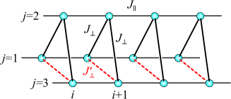
Figure 1: (Color online) Schematic picture of the three-leg tube Hamiltonian (1).

Let us now focus on the case of $s=1/2$ and $J_{\perp}\gg J_{\parallel}$. It is established that the symmetric tube is in the dimer phase and has a finite excitation gap. On the other hand, the system is equivalent to a three-leg ladder in the asymmetric limit $J^{\prime}_{\perp}\rightarrow 0$, and is divided to a single chain and a two-leg ladder in the opposite asymmetric limit $J^{\prime}_{\perp}\rightarrow\infty$; they are both in a gapless critical phase. Therefore, a phase transition between the gapped and gapless phases is naturally expected at some value of $|J^{\prime}_{\perp}-J_{\perp}|>0$.

Surprisingly, it was found Sakai et al. (2005); Nishimoto and Arikawa (2008) that the gap quickly vanishes once the asymmetry is introduced by changing $J^{\prime}_{\perp}$ away from $J_{\perp}$. This is the case in particular in the strong rung-coupling limit $J_{\perp}\gg J_{\parallel}$. In Ref. Nishimoto and Arikawa, 2008, a DMRG calculation revealed that, the gap already collapses with the asymmetry of just one percent $|J^{\prime}_{\perp}-J_{\perp}|/J_{\perp}\sim 1/100$ at $J_{\parallel}/J_{\perp}=1/100$. It appears from the numerical result as if the gap is non-zero only at the symmetric point $J^{\prime}_{\perp}=J_{\perp}$.

However, the conventional wisdom is that any gapped phase extends to a finite range of parameter in any local Hamiltonian. In fact, in Ref. Sakai et al., 2008 non-Abelian bosonization was applied to the three-leg Hubbard model in the ‘band representation’, and it was suggested that the dimer phase remains in a finite range of the asymmetric modulation $|J^{\prime}_{\perp}-J_{\perp}|>0$ and the transition is of the Berezinskii-Kosterlitz-Thouless (BKT) type. They confirmed those theoretical predictions by numerical analyses using DMRG and exact diagonalization, and they also found that the BKT transition is similar to that in the $s=1/2$ $J_{1}$-$J_{2}$ chain. Haldane (1982a); *Haldane82b; Okamoto and Nomura (1992) However, analyzing the effect of the small asymmetric modulation is difficult especially for numerical study. As a consequence, the quantum phase transition between the gapped dimer phase and the gapless phase in the $s=1/2$ three-leg spin tube has not been quantitatively understood. The same system with half-odd-integer $s>1/2$ is even less understood. We note that there are also several studies Charrier et al. (2010); Li et al. (2013) on the three-leg spin tube with integer spin $s$. However, in this paper we focus on half-odd-integer $s$ including the simplest case $s=1/2$.

As an alternative to the analysis of the original spin tube model, an effective Hamiltonian in the strong rung-coupling limit was proposed in Ref. Nishimoto and Arikawa, 2008. This is indeed useful in understanding why the gap vanishes at a small but finite asymmetry. Sakai et al. (2008) However, the effective model has not been studied in detail. In this paper, in order to clarify the nature of phase transitions induced by the rung-coupling modulation in the three-leg spin tube (1) with half-odd-integer spins, we analyze the effective Hamiltonian by field-theoretical and numerical methods.

The paper is organized as follows. In Sec. II.1, we review the derivation of the strong rung-coupling effective Hamiltonian for the $s=1/2$ case and generalize it to arbitrary half-odd-integer spin cases. In Sec. III, the low-energy properties of the effective Hamiltonian are investigated by Abelian bosonization and the renormalization group (RG) analysis. In Sec. IV, the analytical results are confirmed by the level spectroscopy method using exact diagonalization applied to the effective Hamiltonian, and the central charge analysis for the original spin tube using the DMRG method. Finally, we summarize our results in Sec. V.

II Effective Hamiltonian

In this section, we review the derivation Nishimoto and Arikawa (2008) of the strong rung-coupling effective Hamiltonian for the asymmetric tube by using degenerate perturbation theory ($J_{\perp},J^{\prime}_{\perp}\gg J_{\parallel}$). The unperturbed part is the sum of decoupled triangles,

$$H_{0} = \sum_{i}H_{0,i},$$ (2)

$$H_{0,i} = J_{\perp}\left({\vec{s}}_{i,1}\cdot{\vec{s}}_{i,2}+{\vec{s}}_{i,2}\cdot{\vec{s}}_{i,3}\right)+J^{\prime}_{\perp}{\vec{s}}_{i,1}\cdot{\vec{s}}_{i,3}.$$ (3)

We denote the total spin of each triangle, which contains three spin-$s$ sites, as ${\vec{S}}_{i}={\vec{s}}_{i,1}+{\vec{s}}_{i,2}+{\vec{s}}_{i,3}$, and the eigenvalues of ${\vec{S}}_{i}$, $S^{z}_{i}$, and $s_{i,j}^{z}$ respectively as $S$, $M$, and $m_{j}$, where the rung index $i$ is omitted for brevity. For each triangle, basis states diagonalizing $s_{i,j}^{z}$ are denoted as $\left|m_{1}m_{2}m_{3}\right>$. For later convenience, we also introduce the parity $P=\pm 1$ with respect to the exchange of ${\vec{s}}_{i,1}$ and ${\vec{s}}_{i,3}$ in each triangle.

II.1 Spin-$1/2$ case

First, we consider the case of $s=1/2$ ($m_{j}=\uparrow,\downarrow$). This case has been studied for both the symmetric and asymmetric tubes by several groups. Totsuka and Suzuki (1996); Schulz (1996); Nishimoto and Arikawa (2008); Sakai et al. (2008)

Let us begin by analyzing the decoupled triangle (3), which has one quartet and two doublets. Energy of the quartet is $E=\frac{J_{\perp}}{2}+\frac{J^{\prime}_{\perp}}{4}$ and the eigenstates are written as

$$\left|\uparrow\uparrow\uparrow\right>,$$

$$\frac{1}{\sqrt{3}}\left(\left|\uparrow\uparrow\downarrow\right>+\left|\uparrow\downarrow\uparrow\right>+\left|\downarrow\uparrow\uparrow\right>\right),$$

$$\frac{1}{\sqrt{3}}\left(\left|\downarrow\downarrow\uparrow\right>+\left|\downarrow\uparrow\downarrow\right>+\left|\uparrow\downarrow\downarrow\right>\right),$$

$$\left|\downarrow\downarrow\downarrow\right>.$$ (4)

These states have $S=3/2$ and $P=+1$. Since we focus on the antiferromagnetic couplings in this paper, these higher energy states are neglected in the strong rung-coupling limit. The remaining $S=1/2$ doublets are given by

$$\frac{1}{\sqrt{6}}\left(\left|\uparrow\uparrow\downarrow\right>-2\left|\uparrow\downarrow\uparrow\right>+\left|\downarrow\uparrow\uparrow\right>\right)\equiv\left|\uparrow+\right>,$$

$$\frac{1}{\sqrt{6}}\left(\left|\downarrow\downarrow\uparrow\right>-2\left|\downarrow\uparrow\downarrow\right>+\left|\uparrow\downarrow\downarrow\right>\right)\equiv\left|\downarrow+\right>,$$ (5)

with $E=-J_{\perp}+\frac{J^{\prime}_{\perp}}{4}$ and $P=+1$, and

$$\frac{1}{\sqrt{2}}\left(\left|\uparrow\uparrow\downarrow\right>-\left|\downarrow\uparrow\uparrow\right>\right)\equiv\left|\uparrow-\right>,$$

$$\frac{1}{\sqrt{2}}\left(\left|\downarrow\downarrow\uparrow\right>-\left|\uparrow\downarrow\downarrow\right>\right)\equiv\left|\downarrow-\right>,$$ (6)

with $E=-\frac{3J^{\prime}_{\perp}}{4}$ and $P=-1$. These four states are adopted as the unperturbed states. Hereafter, we denote the doublet states as $\left|MP\right>$, where $M=\uparrow,\downarrow$ and $P=+,-$.

By projecting Eq. (1) onto the $4^{L}$-dimensional Hilbert space consisting of the direct products of $\left|MP\right>$’s, the effective Hamiltonian is obtained as

$$H = \frac{J_{\parallel}}{3}\sum_{i=1}^{L}{\vec{S}}_{i}\cdot{\vec{S}}_{i+1}\left[1+8\left(\tau^{x}_{i}\tau^{x}_{i+1}+\tau^{z}_{i}\tau^{z}_{i+1}\right)\right]$$ (7)

$$+\left(J^{\prime}_{\perp}-J_{\perp}\right)\sum_{i=1}^{L}\tau^{z}_{i},$$

up to first order of $J_{\parallel}$, where ${\vec{S}}_{i}$ is the spin-$1/2$ operator at site $i$. The effective model is defined on a 1D chain, where each site $i$ represents three sites on the same rung in the original tube model. Here, the parity operators $\tau^{x,y,z}$ are introduced as

$$\tau^{z}=\frac{1}{2}\left(\left|+\right>\left<+\right|-\left|-\right>\left<-\right|\right),$$ (8)

and

$$\tau^{x}\equiv\frac{1}{2}\left(\tau^{+}+\tau^{-}\right),\hskip 10.0pt\tau^{y}\equiv\frac{1}{2i}\left(\tau^{+}-\tau^{-}\right),$$ (9)

with

$$\tau^{+}=\left|+\right>\left<-\right|,\hskip 10.0pt\tau^{-}=\left|-\right>\left<+\right|,$$ (10)

so that their eigenvalues become $\pm 1/2$ (a half of $P$) as usual spin-$1/2$ operators. By applying an appropriate unitary transformation, the Hamiltonian (7) can be rewritten as

$$H = \frac{J_{\parallel}}{3}\sum_{i=1}^{L}{\vec{S}}_{i}\cdot{\vec{S}}_{i+1}\left[1+8\left(\tau^{x}_{i}\tau^{x}_{i+1}+\tau^{y}_{i}\tau^{y}_{i+1}\right)\right]$$ (11)

$$+\left(J^{\prime}_{\perp}-J_{\perp}\right)\sum_{i=1}^{L}\tau^{x}_{i}.$$

The last term works like a transverse crystal field and its coefficient corresponds to the energy difference between the odd- and even-parity states of the doublets in the unperturbed part.

For the symmetric case ($J^{\prime}_{\perp}=J_{\perp}$), the last term of Eq. (11) vanishes and the effective Hamiltonian is simplified as obtained in the preceding studies. Totsuka and Suzuki (1996); Schulz (1996) We thus can regard $\tau$ as an operator acting on chirality corresponding to momenta $\pm 2\pi/3$ in the rung triangle, and spin and chirality are coupled by the leg exchange interaction in a biquadratic form. It has been confirmed that the system is in a spontaneously dimerized state where the spin and chirality form singlet pairs alternately and have a finite excitation gap. Kawano and Takahashi (1997)

For the asymmetric case ($J^{\prime}_{\perp}\neq J_{\perp}$), while the effective model (11) was derived in Ref. Nishimoto and Arikawa, 2008, no definitive study has been so far reported. We here start from trivial limits. If the transverse field is sufficiently strong, the chirality degrees of freedom are fully polarized, and the Hamiltonian (11) is reduced to the spin-$1/2$ Heisenberg chain. Hence, the system goes to a gapless critical phase. In the original spin tube (1) with $s=1/2$, these limits correspond to a three-leg open ladder ($J^{\prime}_{\perp}-J_{\perp}\rightarrow-J_{\perp}$) and a decoupled system consisting of a single chain and a two-leg ladder ($J^{\prime}_{\perp}-J_{\perp}\rightarrow\infty$), respectively. In both of these limits, the original spin tube model is gapless. Thus the effective model correctly describes the origninal spin tube in these limits. We can further expect that the phase transitions between the dimer and critical phases are also described by the effective Hamiltonian (11). It is the purpose of the present paper to elucidate the phase transitions in detail, based on the effective Hamiltonian.

II.2 General-$s$ case

Next, we consider the general half-odd-integer spin-$s$ cases. A similar analysis for the decoupled triangle with integer spin was also done in Ref. Charrier et al., 2010. The Hamiltonian (3) can be expressed as

$$H_{0,i} = \frac{J_{\perp}}{2}{\vec{S}}^{2}+\frac{J^{\prime}_{\perp}-J_{\perp}}{2}{\vec{S}}_{13}^{2}-\frac{J_{\perp}}{2}{\vec{s}}_{2}^{2}-\frac{J^{\prime}_{\perp}}{2}\left({\vec{s}}_{1}^{2}+{\vec{s}}_{3}^{2}\right)$$ (12)

$$= \frac{J_{\perp}}{2}S\left(S+1\right)+\frac{J^{\prime}_{\perp}-J_{\perp}}{2}S_{13}\left(S_{13}+1\right)$$

$$-\frac{J_{\perp}+2J^{\prime}_{\perp}}{2}s\left(s+1\right),$$

where we omitted the rung index $i$ for simplicity. We also defined the total spin $\vec{S}=\vec{s}_{1}+\vec{s}_{2}+\vec{s}_{3}$ and the bond spin ${\vec{S}}_{jk}={\vec{s}}_{j}+{\vec{s}}_{k}$, and their magnitudes $S$ and $S_{jk}$ by $\vec{S}^{2}=S(S+1)$ and ${\vec{S}_{jk}}^{2}=S_{jk}(S_{jk}+1)$. For the symmetric case ($J^{\prime}_{\perp}=J_{\perp}$), the ground state belongs to the $S=1/2$ sector for any half-odd-integer spin-$s$. From the composition rule of angular momentum, $S_{13}$ obeys $S_{13}=s\pm 1/2$ and the ground state is four-fold degenerate with respect to $S_{13}$ and the eigenvalue $M=\pm 1/2$ of $S^{z}$. If we introduce a finite modulation of the rung couplings ($J^{\prime}_{\perp}\neq J_{\perp}$), degeneracy corresponding to $S_{13}$ is lifted. At some modulation $J^{\prime}_{\perp}-J_{\perp}$, the energy level of the $S=1/2$ doublet ground state meets that of an $S=3/2$ quadruplet. For higher spin cases ($s>1/2$), the ground state belongs to an $S=1/2$ doublet only in the restricted range of the modulation,

$$\frac{2s}{2s+3}<\frac{J^{\prime}_{\perp}}{J_{\perp}}<\frac{2\left(s+1\right)}{2s-1},$$ (13)

centered around the symmetric point $J^{\prime}_{\perp}/J_{\perp}=1$. Since the bond spin $S_{13}$ is related to the parity for exchanging between ${\vec{s}}_{1}$ and ${\vec{s}}_{3}$, we can derive the effective Hamiltonian for $s>1/2$ by following the same procedure as in the $s=1/2$ case. The detailed calculations are available in the Appendix. As a result, the effective Hamiltonian for general half-odd-integer spin-$s$ is given by

$$H = \frac{J_{\parallel}}{3}\sum_{i=1}^{L}{\vec{S}}_{i}\cdot{\vec{S}}_{i+1}\left[1+2\alpha\left(\tau^{x}_{i}\tau^{x}_{i+1}+\tau^{y}_{i}\tau^{y}_{i+1}\right)\right]$$ (14)

$$+h\sum_{i=1}^{L}\tau^{x}_{i},$$

where

$$\alpha=\left(2s+1\right)^{2},\hskip 10.0pth=\frac{2s+1}{2}\left(J^{\prime}_{\perp}-J_{\perp}\right).$$ (15)

This effective Hamiltonian for general half-odd integer $s$ has the same form as that (11) for $s=1/2$, and the $s$-dependence only enters through the coupling constants $\alpha$ and $h$. However, it should be noted that this effective Hamiltonian is only valid in the range (13). This Hamiltonian coincides also with the one obtained for the three-leg spin tube with a finite magnetization, Plat et al. (2012) if $h=0$ and ${\vec{S}}_{i}\cdot{\vec{S}}_{i+1}$ is taken as a constant. The parameter $h$ corresponds to the strength of the asymmetry. For the symmetric case ($h=0$), earlier DMRG studies Kawano and Takahashi (1997); Lüscher et al. (2004) have confirmed that the ground state is in the dimer phase for any value of $\alpha$. Therefore, it is safe to say that the general half-odd-integer spin-$s$ tube exhibits the dimer phase at $h=0$ in the strong rung-coupling limit. This is consistent with the DMRG calculations Nishimoto et al. (2011); Plat et al. (2012) for the $s=3/2$ tube ($\alpha=16$) as well as those Schnack et al. (2004); Fouet et al. (2006) on the $s=1/2$ ‘twisted’ tube ($\alpha=2$).

II.3 Relationship with the spin-orbital model

It is worth mentioning known models related to the effective Hamiltonian (14). Indeed, it can be recognized to be a special form of the spin-orbital models which were first derived for the strong-coupling limit of the two-band Hubbard model at quarter-filling. Kugel and Khomskii (1982) If the parameters of the spin-orbital model are tuned in an appropriate way, we obtain the following Hamiltonian,

$$H = \sum_{i=1}^{L}\left[J_{1}{\vec{S}}_{i}\cdot{\vec{S}}_{i+1}+J_{2}\left(T^{x}_{i}T^{x}_{i+1}+T^{y}_{i}T^{y}_{i+1}\right)\right.$$ (16)

$$\left.+K\left({\vec{S}}_{i}\cdot{\vec{S}}_{i+1}\right)\left(T^{x}_{i}T^{x}_{i+1}+T^{y}_{i}T^{y}_{i+1}\right)\right],$$

where ${\vec{T}}_{i}$ is the orbital SU(2) matrix at site $i$. We observe that the model (16) reduces to the effective Hamiltonian (14) with $h=0$, if $J_{1}=J_{\parallel}/3$, $J_{2}=0$, and $K=2\alpha J_{\parallel}/3$. Hence, our effective Hamiltonian takes the same form as Eq. (16) by adding an extra chirality chain and turning off the transverse field. The system (16) has been studied by several groups. Orignac et al. (2000); Pati and Singh (2000); Kolezhuk et al. (2001) At $J_{1}/K=3/4$ and $J_{2}/K=1/2$, it is exactly solvable and the ground state is in a spontaneously dimerized phase where spin and orbital form singlets alternatively along the chain. Pati and Singh (2000); Kolezhuk et al. (2001) As shown in the phase diagram of Ref. Pati and Singh, 2000, the dimer phase is extended to a wide parameter space for $J_{1}>0$, except for some $J_{2}>J_{1}$ region where the ground state is composed of a spin ferromagnet and an orbital Fermi sea. Also, the possibility of the first order transition was suggested in the $J_{1}>0,J_{2}>0$ region; on the other hand, the dimer phase seems to be smoothly connected to the $J_{2}=0$ line, which corresponds to our effective Hamiltonian (14), from the $J_{1}>0,J_{2}<0$ region.

We here mention a relation between the spin-orbital model (16) and the spin tube (1) with ferromagnetic legs. For the symmetric spin tube with ferromagnetic legs, the corresponding effective Hamiltonian is again described by Eq. (14) with $J_{\parallel}<0$ and $h=0$. In Ref. Pati and Singh, 2000, this Hamiltonian has also been studied in the context of the spin-orbital model (16), and its ground state is still in a dimer phase for $\alpha>2$. This result is consistent with a DMRG study in the $s=1/2$ spin tube with ferromagnetic legs, and a dimer phase is extended beyond the strong rung-coupling regime. Nishimoto and Arikawa (2010)

III Field theoretical analysis

In this section, we analyze the effective Hamiltonian (14) with a field theoretical method. The bosonization approach combined with the RG method is a very powerful and successful tool to study the low-energy properties of 1D systems. Gogolin et al. (1998); Giamarchi (2003) In this paper, Abelian bosonization is adopted. We first divide the effective Hamiltonian (14) into a single spin chain ($H_{S}$) and interaction between the two degrees of freedom ($H_{I}$):

$$H=H_{S}+H_{I},$$ (17)

where

$$H_{S} = J_{s}\sum_{i=1}^{L}{\vec{S}}_{i}\cdot{\vec{S}}_{i+1},$$

$$H_{I} = \lambda\sum_{i=1}^{L}{\vec{S}}_{i}\cdot{\vec{S}}_{i+1}\left(\tau^{x}_{i}\tau^{x}_{i+1}+\tau^{y}_{i}\tau^{y}_{i+1}\right)+h\sum_{i=1}^{L}\tau^{x}_{i}.$$

Comparing (17) with Eq. (14), the couplings constants are identified as $J_{s}=J_{\parallel}/3$ and $\lambda=2J_{\parallel}\alpha/3$. The case of $h=0$ was studied in Ref. Orignac et al., 2000. We extend their bosonization approach in the presence of the transverse field on chirality and derive a low-energy effective theory which describes the phase transition in the spin tube (1).

III.1 Bosonization

Let us start with the single spin chain $H_{S}$. In the continuum limit, the bosonized Hamiltonian is given by

$$H_{S} \approx \frac{v_{s}}{2\pi}\int dx\left[K_{s}\left(\partial_{x}\theta_{s}\right)^{2}+\frac{1}{K_{s}}\left(\partial_{x}\phi_{s}\right)^{2}\right]$$ (18)

$$-\frac{2g_{0}}{\left(2\pi a_{0}\right)^{2}}\int dx\cos\left(\sqrt{8}\phi_{s}\right),$$

where $x=a_{0}i$ ($a_{0}$: lattice spacing) and $g_{0}$ is a positive constant. We here introduce the dual field for spin, satisfying the commutation relation,

$$\left[\phi_{s}(x),\theta_{s}(x^{\prime})\right]=-\frac{i\pi}{2}{\rm sgn}(x-x^{\prime}).$$

For an isolated spin chain, the velocity $v_{s}$ and the Luttinger parameter $K_{s}$ are exactly determined via Bethe ansatz: Giamarchi (2003); Orignac et al. (2000) $v_{s}=\pi J_{s}a_{0}/2$, $K_{s}=1$. Although the last term in Eq. (18) is marginally irrelevant and gives logarithmic corrections to various finite-size quantities, the low-energy properties of $H_{S}$ are described by a Tomonaga-Luttinger liquid (TLL) which is critical and gapless. However, if the interactions between spin and chirality are present, the $\cos(\sqrt{8}\phi_{s})$ term plays a crucial role and could induce the phase transition. Thus, we keep this term in the following analysis.

Unlike the spin-orbital model (16), our Hamiltonian (17) originally does not contain a single chirality chain. However, as pointed out in Ref. Orignac et al., 2000, the interaction part $H_{I}$ can produce a finite velocity of chirality through the ‘mean-field-like’ contribution. To see this, we split the nearest-neighbor spin correlation operator into the expectation value with respect to the ground state of $H_{S}$, $\left<{\vec{S}}_{i}\cdot{\vec{S}}_{i+1}\right>_{0}$, and the remaining “normal-ordered” part, $:{\vec{S}}_{i}\cdot{\vec{S}}_{i+1}:$, as

$${\vec{S}}_{i}\cdot{\vec{S}}_{i+1}=:{\vec{S}}_{i}\cdot{\vec{S}}_{i+1}:+\left<{\vec{S}}_{i}\cdot{\vec{S}}_{i+1}\right>_{0}.$$ (19)

Therefore, one can see that the interaction part $H_{I}$ gives a single chirality chain part, $-J_{c}\left(\tau^{x}_{i}\tau^{x}_{i+1}+\tau^{y}_{i}\tau^{y}_{i+1}\right)$, with a finite ferromagnetic exchange coupling $-J_{c}=\lambda\left<{\vec{S}}_{i}\cdot{\vec{S}}_{i+1}\right>_{0}<0$. Like in a mean-field theory, chirality also gives a finite contribution to the spin chain through a similar decoupling as in Eq. (19). However, considering $\lambda$ as a perturbation, the mean-field-like contribution merely provides small corrections to $v_{s}$ and $K_{s}$; furthermore, the SU(2) symmetry for spin ensures that $K_{s}$ stays at unity. Therefore, we neglect such corrections and suppose that they do not affect the qualitative properties of Eq. (17) as long as we keep $\lambda$ as a perturbation.

To obtain a bosonized form of $H_{I}$, we introduce the bosonization formulas for spin and chirality. In our bosonization language, spin operators are given by

$$S^{z}_{i}\approx\frac{a_{0}}{\pi\sqrt{2}}\partial_{x}\phi_{s}+b(-1)^{i}\cos(\sqrt{2}\phi_{s}),$$ (20)

$$S^{+}_{i}\approx e^{i\sqrt{2}\theta_{s}}\left[b(-1)^{i}+{\frac{1}{\pi}}\cos(\sqrt{2}\phi_{s})\right],$$ (21)

where $b$ is a nonuniversal constant which can be numerically evaluated. Lukyanov (1998); Hikihara and Furusaki (1998); Takayoshi and Sato (2010) Similarly, chirality operators are given by

$$\tau^{+}_{i}\approx\frac{e^{i\sqrt{2}\theta_{c}}}{\sqrt{2\pi}}\left[1+(-1)^{i}\cos(\sqrt{2}\phi_{c})\right],$$ (22)

where $\phi_{c}$ and $\theta_{c}$ satisfy the commutation relation,

$$\left[\phi_{c}(x),\theta_{c}(x^{\prime})\right]=-\frac{i\pi}{2}{\rm sgn}(x-x^{\prime}).$$

They are obtained in a standard manner through the Jordan-Wigner transformation. Giamarchi (2003) The staggered parts of the (normal-ordered) nearest-neighbor correlations are also given by

$$(-1)^{i}:{\vec{S}}_{i}\cdot{\vec{S}}_{i+1}:\approx d\sin(\sqrt{2}\phi_{s})$$ (23)

for spin, and

$$(-1)^{i}:\tau^{x}_{i}\tau^{x}_{i+1}+\tau^{y}_{i}\tau^{y}_{i+1}:\approx-\frac{1}{\pi}\sin(\sqrt{2}\phi_{c})$$ (24)

for chirality. The coefficient $d$ is a non-universal positive constant and has so far been obtained by several groups. Takayoshi and Sato (2010); Orignac (2004) The staggered parts of chirality correlations (24) are also evaluated via the Jordan-Wigner transformation. Orignac et al. (2000); Orignac and Giamarchi (1998) In the above formulas, we have neglected the higher-order terms because they only give irrelevant perturbations to the low-energy physics in most cases. Using Eqs. (20) to (24), the perturbation $H_{I}$ can be expressed in terms of boson fields as

$$H_{I} \approx \frac{v_{c}}{2\pi}\int dx\left[K_{c}(\partial_{x}\theta_{c})^{2}+\frac{1}{K_{c}}(\partial_{x}\phi_{c})^{2}\right]$$ (25)

$$-\frac{\lambda d}{\pi a_{0}}\int dx\sin(\sqrt{2}\phi_{s})\sin(\sqrt{2}\phi_{c})$$

$$+\frac{h}{\sqrt{2\pi}a_{0}}\int dx\cos(\sqrt{2}\theta_{c}),$$

where $v_{c}=J_{c}a_{0}$ and $K_{c}=2$.

Finally, we obtain the bosonized form of the full Hamiltonian (17),

$$H \approx \sum_{\nu=s,c}\frac{v_{\nu}}{2\pi}\int dx\left[K_{\nu}\left(\partial_{x}\theta_{\nu}\right)^{2}+\frac{1}{K_{\nu}}\left(\partial_{x}\phi_{\nu}\right)^{2}\right]$$ (26)

$$-\frac{2g_{0}}{(2\pi a_{0})^{2}}\int dx\cos(\sqrt{8}\phi_{s})$$

$$-\frac{2g_{1}}{(2\pi a_{0})^{2}}\int dx\sin(\sqrt{2}\phi_{s})\sin(\sqrt{2}\phi_{c})$$

$$+\frac{2g_{2}}{(2\pi a_{0})^{2}}\int dx\cos(\sqrt{2}\theta_{c}),$$

where the coupling constants are given by

$$g_{1}=2\pi a_{0}\lambda d,\hskip 10.0pt g_{2}=\sqrt{2\pi^{3}}a_{0}h.$$ (27)

In this Hamiltonian, both $g_{1}$ and $g_{2}$ are relevant since their scaling dimensions are given by $(K_{s}+K_{c})/2\sim 3/2$ and $1/(2K_{c})\sim 1/4$, respectively. To investigate the low-energy physics, we perform the perturbative RG analysis in the following section.

III.2 Renormalization group equations

Using the operator product expansion, Cardy (1996) we obtain the following RG equations,

$$\frac{dy_{0}}{dl} = \left(2-K_{s}\right)y_{0}-\frac{1}{8}y_{1}^{2},$$ (28a)

$$\frac{dy_{1}}{dl} = \left(2-\frac{K_{s}+K_{c}}{2}\right)y_{1}+\frac{1}{2}y_{0}y_{1},$$ (28b)

$$\frac{dy_{2}}{dl} = \left(2-\frac{1}{2K_{c}}\right)y_{2},$$ (28c)

$$\frac{dK_{s}}{dl} = -\frac{1}{2}K_{s}^{2}y_{0}^{2}-\frac{1}{16}K_{s}^{2}y_{1}^{2},$$ (28d)

$$\frac{dK_{c}}{dl} = -\frac{1}{16}K_{c}^{2}y_{1}^{2}+\frac{1}{8}y_{2}^{2},$$ (28e)

where $l$ is the logarithmic length scale. In these equations, the velocity difference between spin and chirality chains is neglected, i.e., $u\equiv v_{s}=v_{c}$, and we set $y_{i}=g_{i}/(\pi u)$, for simplicity.

Let us first consider the symmetric tube ($g_{2}=0$), which has been studied with the RG method in Ref. Orignac et al., 2000. In this case, only $g_{1}$ is relevant and the ground-state energy is minimized when the condition

$$\sin(\sqrt{2}\phi_{s})\sin(\sqrt{2}\phi_{c})=1$$ (29)

is satisfied. Then, the field for spin (chirality) is locked to $\phi_{s}=\pi/\sqrt{8}$ ($\phi_{c}=\pi/\sqrt{8}$) or $\phi_{s}=-\pi/\sqrt{8}$ ($\phi_{c}=-\pi/\sqrt{8}$), and the dimer order parameters for both spin and chirality have finite expectation values from Eqs. (23) and (24). This indicates the presence of a long-range dimer order, in agreement with the previous DMRG calculations. Kawano and Takahashi (1997); Lüscher et al. (2004) In this phase, the spin and chirality form singlets on bonds alternatively and translational symmetry is spontaneously broken. Consequently, both spin and chirality excitations are gapped.

Next we introduce the asymmetry of the rung triangle ($g_{2}\neq 0$). In the limit of $|g_{2}|\to\infty$, the chirality degrees of freedom are completely frozen out and only spin degrees of freedom remain; therefore, the system is in a TLL phase. The coupling $g_{2}$ is highly relevant and it would be expected that the chirality is polarized along the $x$-direction as soon as $g_{2}$ is switched on. However, the other coupling $g_{1}$ competes with $g_{2}$ because $g_{1}$ pins the field $\phi_{c}$ whereas $g_{2}$ pins its dual field $\theta_{c}$. Thus, a finite critical value of $g_{2c}$ to bring the system from the dimer-ordered state to another one may exist. We will discuss this possibility in more detail in the next subsection.

III.3 Effective theory for the spin degrees of freedom

In this subsection, we derive an effective theory only for the spin degrees of freedom, which describes the transition between the dimer and TLL phases, in the case of sufficiently strong $g_{2}$. Here, we apply the two-cutoff scaling method. Gogolin et al. (1998); Kim and Sólyom (1999) The coupling $g_{2}$, the initial value of which is $g_{2}(l=0)\propto h$, is the most relevant perturbation at the weak-coupling fixed point (two-component TLL of spin and chirality). Thus we assume that, while $g_{2}$ grows to $O(1)$, other couplings remain perturbatively small under the RG. We define the logarithmic length scale $\bar{l}$ such that $g_{2}(l=\bar{l})=O(1)$. At this length scale, the field $\theta_{c}$ is locked to the potential minimum; $\theta_{c}$ and its dual $\phi_{c}$ can be safely integrated out as massive fields.

The partition function is written as

$${\mathcal{Z}}=\int{\mathcal{D}}\phi_{s}{\mathcal{D}}\phi_{c}e^{-S_{0}[\phi_{s}]-S_{c}[\phi_{c}]-S_{1}[\phi_{s},\phi_{c}]},$$ (30)

where

$$S_{0}[\phi_{s}] = \frac{u}{2\pi{\bar{K}}_{s}}\int d^{2}r\left[\frac{1}{u^{2}}(\partial_{\tau}\phi_{s})^{2}+(\partial_{x}\phi_{s})^{2}\right],$$ (31)

$$S_{c}[\phi_{c}] = \frac{u}{2\pi{\bar{K}}_{c}}\int d^{2}r\left[\frac{1}{u^{2}}(\partial_{\tau}\phi_{c})^{2}+(\partial_{x}\phi_{c})^{2}\right]$$ (32)

$$+\frac{2{\bar{g}}_{2}}{(2\pi a_{0})^{2}}\int d^{2}r\cos(\sqrt{8}\theta_{c}),$$

$$S_{1}[\phi_{s},\phi_{c}] = \frac{2}{(2\pi a_{0})^{2}}\int d^{2}r\left[-{{\bar{g}}_{0}}\cos(\sqrt{8}\phi_{s})\right.$$ (33)

$$\left.+{\bar{g}}_{1}\sin(\sqrt{2}\phi_{s})\sin(\sqrt{2}\phi_{c})\right],$$

and ${\bar{X}}=X(l={\bar{l}})$ denotes a renormalized coupling and $r\equiv(\tau,x)$. We expand the partition function up to second order in $S_{1}$,

$${\mathcal{Z}}=z_{c}\int{\mathcal{D}}\phi_{s}e^{-S_{0}[\phi_{s}]}\left[1-\left<S_{1}\right>_{c}+\frac{1}{2}\left<S_{1}^{2}\right>_{c}+\cdots\right],$$ (34)

where the expectation value is defined by

$$\left<\cdots\right>_{c}=\frac{1}{z_{c}}\int{\mathcal{D}}\phi_{c}(\cdots)e^{-S_{c}[\phi_{c}]},$$ (35)

and $z_{c}=\int{\mathcal{D}}\phi_{c}e^{-S_{c}[\phi_{c}]}$ is a constant. The first order contribution is easily evaluated as

$$\left<S_{1}\right>_{c}=-\frac{2{{\bar{g}}_{0}}}{(2\pi a_{0})^{2}}\int d^{2}r\cos(\sqrt{8}\phi_{s}).$$ (36)

A non-vanishing term in the second order contribution is given by

$$\left<S_{1}^{2}\right>_{c} = \frac{4{\bar{g}}_{1}^{2}}{(2\pi a_{0})^{4}}\int d^{2}r_{1}d^{2}r_{2}$$ (37)

$$\times\sin\left(\sqrt{2}\phi_{s}(r_{1})\right)\sin\left(\sqrt{2}\phi_{s}(r_{2})\right)$$

$$\times\left<\sin\left(\sqrt{2}\phi_{c}(r_{1})\right)\sin\left(\sqrt{2}\phi_{c}(r_{2})\right)\right>_{c}.$$

Since the field $\theta_{c}$ is ordered in the present case, its dual field $\phi_{c}$ is disordered and the correlation function of $\phi_{c}$ decays exponentially. Thus, we consider only the short-range contribution from $r_{1}\sim r_{2}$ and approximate as follows:

$$\left<\sin\left(\sqrt{2}\phi_{c}(r_{1})\right)\sin\left(\sqrt{2}\phi_{c}(r_{2})\right)\right>_{c}\approx D\delta(r_{1}-r_{2}),$$ (38)

where $D$ is a positive nonuniversal constant. Then, Eq. (37) is rewritten as

$$\left<S_{1}^{2}\right>_{c}\approx-\frac{2D{\bar{g}}_{1}^{2}}{(2\pi a_{0})^{2}}\int d^{2}r\cos(\sqrt{8}\phi_{s}).$$ (39)

Further, we reexponentiate the expectation values in Eq. (34) and obtain the effective action,

$$S_{\rm eff}[\phi_{s}]=S_{0}[\phi_{s}]-\frac{2{\bar{g}}_{0}-D{\bar{g}}_{1}^{2}}{(2\pi a_{0})^{2}}\int d^{2}r\cos(\sqrt{8}\phi_{s}),$$ (40)

where ${\mathcal{Z}}\approx z_{c}\int{\mathcal{D}}\phi_{s}e^{-S_{\rm eff}[\phi_{s}]}$.

Finally, the effective spin Hamiltonian above the scale ${\bar{l}}$ is given by the usual sine-Gordon model,

$$H_{\rm eff} = \frac{u}{2\pi}\int dx\left[{\bar{K}}_{s}(\partial_{x}\theta_{s})^{2}+\frac{1}{{\bar{K}}_{s}}(\partial_{x}\phi_{s})^{2}\right]$$ (41)

$$-\frac{2G}{(2\pi a_{0})^{2}}\int dx\cos(\sqrt{8}\phi_{s}),$$

where $G={{\bar{g}}_{0}}-D{\bar{g}}_{1}^{2}/2$.

Although this Hamiltonian does not contain explicitly the transverse field $h$ in the original model, it does depend on $h$. This is because the length scale $\bar{l}$ and thus the renormalized couplings at $l=\bar{l}$ are determined by $g_{2}(l=0)\propto h$. In the leading approximation, $\bar{l}\propto-\frac{1}{2-1/(2K_{c})}\log{h}\sim-\frac{4}{7}\log{h}$, $\bar{g}_{0}\sim g_{0}$, and $\bar{g}_{1}\sim g_{1}\exp{\left[(2-\frac{K_{s}+K_{c}}{2})\bar{l}\right]}\sim g_{1}h^{-2/7}$. Inclusion of subleading terms in the RG equation changes these values, although the qualitative picture remains the same as long as $\bar{g}_{0}$ and $\bar{g}_{1}$ are small. On the other hand, thanks to the SU(2) symmetry, ${\bar{K}}_{s}$ should be always 1. The sine-Gordon interaction in the last term of Eq. (41) has the scaling dimension $2$ and thus is marginal. In fact, it is marginally relevant or irrelevant, depending on the sign of $G$. If $h$ is sufficiently strong, ${\bar{g}}_{1}$ does not change much from its initial value $g_{1}(l=0)$ and $G$ stays positive; the system is in a TLL phase with a marginally irrelevant term. If $h$ decreases, $g_{1}$ grows under the RG flow and $G$ can be negative. In this case, $G$ is marginally relevant and $\phi_{s}$ is locked into one of its minima $\pm\pi/\sqrt{8}$; the system goes into a dimer phase. Therefore, at a critical value of $h$ where the marginal coupling $G$ exactly vanishes, we can expect a phase transition between the TLL and dimer phases. This belongs to a particular variant of BKT transition with the SU(2) symmetry in the entire region, as known in the $s=1/2$ $J_{1}$-$J_{2}$ chain. Affleck et al. (1989); Okamoto and Nomura (1992) We check these expectations numerically in the following section.

IV Numerical analysis

In this section, we attempt to confirm numerically the above picture obtained from the analytical arguments. First we verify the phase transition in the effective Hamiltonian (14) numerically, based on the level spectroscopy method with exact diagonalization. Furthermore, we also look for the phase transition in the original spin tube model by numerical estimation of central charge with DMRG. Hereafter, we focus on the $s=1/2$ case and set $J_{\parallel}=1$ as energy unit unless otherwise stated.

IV.1 Level Spectroscopy for the effective Hamiltonian

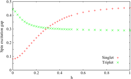
Figure 2: (Color Online) Excitation spectra for the model (14) with $s=1/2$, $L=16$, as functions of $h$. Symbols $+$ and $\times$ denote the singlet-singlet and singlet-triplet excitation gaps, respectively.

Here we apply the level spectroscopy method Okamoto and Nomura (1992) to the effective Hamiltonian (14). This enables us to detect the BKT transition between the dimer and TLL phases. Finite-size systems of $L=8$, $10$, $12$, $14$, and $16$ are studied using exact diagonalization technique with the PBC. In the context of the sine-Gordon theory, the gaps of singlet-singlet and singlet-triplet excitations are expected to cross at the BKT transition point for a finite-size system. As an example, the results of the gaps for $L=16$ are shown in FIG. 2. We can clearly see the crossing at $h\simeq 0.24$.

In order to check the universality class of the present BKT transition, we estimate the scaling dimensions. By conformal field theory (CFT), the scaling dimensions are related to the excitation spectra of a finite-size system as follows, Cardy (1984)

$$E_{n}(L)-E_{gs}(L)=\frac{2\pi v}{L}x_{n}(L),$$ (42)

where $E_{n}(L)$ and $E_{gs}(L)$ are energies of an excited state and of the ground state, respectively, for a system with length $L$, $v$ is the spin-wave velocity, and $x_{n}(L)$ is the scaling dimension. The subscript $n$ is an index labeling the type of excitations (see below). In the TLL phase, the scaling dimensions for the first singlet ($n=s$) and triplet ($n=t$) excitations have logarithmic corrections from the marginal perturbation: Affleck et al. (1989)

$$x_{s}(L)=\frac{1}{2}+\frac{3}{4}\frac{1}{\log L}+{\mathcal{O}}\left(\frac{1}{L^{2}}\right),$$ (43)

$$x_{t}(L)=\frac{1}{2}-\frac{1}{4}\frac{1}{\log L}+{\mathcal{O}}\left(\frac{1}{L^{2}}\right).$$ (44)

These logarithmic corrections are expected to vanish only at the BKT transition point. Away from the transition point, they quickly become significant and often cause severe problems to scaling analyses. It is thus very useful to remove the corrections by taking an average $x_{a}=(x_{s}+3x_{t})/4$. Ziman and Schulz (1987) To obtain the scaling dimensions, we still need an estimate of the spin-wave velocity $v$. It is typically determined by

$$v(L)=\frac{L}{2\pi}\left[E^{k}(L)-E_{gs}(L)\right],$$ (45)

for a system with length $L$, where $E^{k}(L)$ is an energy of the first-excited state with wave vector $k=2\pi/L$ (the ground state is characterized by $k=0$). We calculate $v(L)$ for $L=8-16$, and then extrapolate it to the thermodynamic limit via a fitting function,

$$v(L)=v+A_{0}\frac{1}{L^{2}}+A_{1}\frac{1}{L^{4}}+\cdots,$$ (46)

where $A_{0}$ and $A_{1}$ are fitting parameters. For all values of $h(<1)$, the fitting works perfectly despite neglecting the higher-order terms. The estimated values of $x_{s}$, $x_{t}$, and $x_{a}$ as functions of $h$ are shown in FIG. 3. The original scaling dimensions $x_{s}$ and $x_{t}$ are near $1/2$ only around the crossing point $h_{\rm cross}$, while $x_{a}$ remains close to $1/2$ at $h\gtrsim h_{\rm cross}$. This indicates that the crossing point corresponds to the BKT transition between the dimer and TLL phases. Note that $h_{\rm cross}$ is equivalent to the crossing point between the singlet-singlet and singlet-triplet gaps shown in FIG. 2. The similar results have also been obtained for the original $s=1/2$ spin tube (1). Sakai et al. (2008)

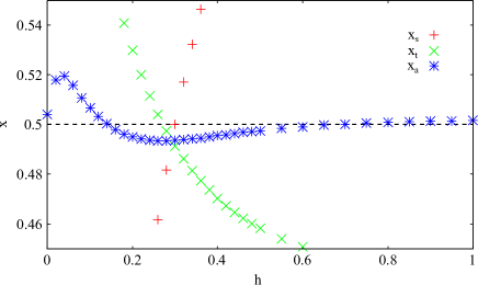
Figure 3: (Color Online) Scaling dimensions fo the model (14) with $s=1/2$, $L=16$, as functions of $h$. Symbols $+$, $\times$, and $+\times$ denote $x_{s}$, $x_{t}$, and $x_{a}$, respectively (see text).

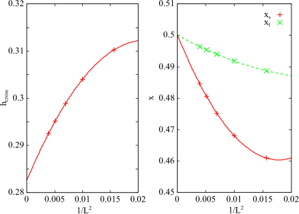
Figure 4: (Color Online) Size scaling of the crossing point between $x_{s}$ and $x_{t}$ (left panel), and of the scaling dimensions at the transition point $h_{c}=0.283$ (right panel), as functions of $1/L^{2}$. In the right panel, symbols $+$ and $\times$ denote $x_{s}$ and $x_{t}$, respectively. Fitting functions (47) and (48) are used for the finite-size scaling.

At the BKT transition, there is no logarithmic correction, but other corrections attributed to the $x=4$ irrelevant perturbation exist. Cardy (1986a, b) Therefore, we extrapolate the crossing point and scaling dimensions to the thermodynamic limit, using the following scaling functions,

$$h_{\rm cross}(L) = h_{c}+B_{0}\frac{1}{L^{2}}+B_{1}\frac{1}{L^{4}}+\cdots,$$ (47)

$$x(L) = x_{c}+C_{0}\frac{1}{L^{2}}+C_{1}\frac{1}{L^{4}}+\cdots,$$ (48)

where $B$’s and $C$’s are fitting parameters. The scaling analyses are shown in FIG. 4. The crossing point in the thermodynamic limit is evaluated as

$$h_{c}=0.283,$$ (49)

which corresponds to the critical value of $h$ between the dimer and TLL phases. We note that the critical point $h_{c}$ is obtained with respect to the leg coupling $J_{\parallel}=1$. It remains finite in the strong rung-coupling limit $J^{\prime}_{\perp},J_{\perp}\to\infty$. Since $h=J^{\prime}_{\perp}-J_{\perp}$, the critical asymmetry ratio $(J^{\prime}_{\perp,c}-J_{\perp})/J_{\perp}$ is small (proportional to $1/J_{\perp}$) in the strong rung-coupling limit $J_{\perp}\rightarrow\infty$.

In Ref. Sakai et al., 2008 and Sakai et al., 2005, Sakai et al. studied the original spin-$1/2$ tube by the level spectroscopy method using exact diagonalization and found the dimer phase in the region $0.95\lesssim J^{\prime}_{\perp}/J_{\perp}\lesssim 1.05$ for $J_{\parallel}/J_{\perp}=0.2$. Although the critical asymmetry in our study, $|J^{\prime}_{\perp}-J_{\perp}|/J_{\parallel}=0.283$, is obtained in the strong-rung coupling limit, this is considerably close to the value $|J^{\prime}_{\perp}-J_{\perp}|/J_{\parallel}\sim 0.25$ obtained by Sakai et al. Thus the present work strongly supports that a finite but small critical asymmetry exists in the strong rung-coupling region.

At $h=h_{c}$, both the singlet and triplet scaling dimensions are extrapolated to $x_{c}=0.500$ in the thermodynamic limit. This is consistent with the theoretical prediction, giving a strong evidence supporting the theory developed in Sec. III. Our analysis in this section is limited to the value of $\alpha$ in Eq. (15) corresponding to $s=1/2$. Nevertheless, from Eq. (14), it is easily speculated that essentially the same BKT transition occurs for the general-$s$ ($s\geq 1/2$) cases, i.e., for any $\alpha$, in the strong rung-coupling regime since $\alpha$ changes only the strength of coupling between the spin and chirality chains.

IV.2 DMRG for the three-leg spin tube

In order to confirm the validity of the analysis based on the effective Hamiltonian, here we investigate the transition point in the original spin tube (1) by calculating the central charge using the DMRG method. White (1992); Schollwöck (2005)

The central charge, which can be evaluated via the von-Neumann entanglement entropy, gives a direct information to determine the universality classes of 1D quantum systems. From CFT, the von-Neumann entanglement entropy of a subsystem with length $l$ in a periodic system with length $L$ has the following scaling form, Calabrese and Cardy (2004)

$$S_{L}(l)=\frac{c}{3}\ln\left[\frac{L}{\pi}\sin\left(\frac{\pi l}{L}\right)\right]+c^{\prime},$$ (50)

for a critical phase, where $c$ is the central charge and $c^{\prime}$ is a nonuniversal constant. Using this formula, we estimate $c$ as Nishimoto (2011)

$$c(L)=\frac{3\left[S_{L}\left(\frac{L}{2}-1\right)-S_{L}\left(\frac{L}{2}\right)\right]}{\ln\left[\cos\left(\frac{\pi}{L}\right)\right]}.$$ (51)

In the thermodynamic limit, the central charge is $c=1$ for the gapless TLL phase while $c=0$ for the gapped dimer phase.

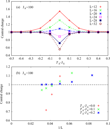
Figure 5: (Color Online) (a) Central charge of the $s=1/2$ three-leg spin tube (1) with $J_{\perp}=100$, as functions of $J^{\prime}_{\perp}-J_{\perp}$. (b) System-size dependence of the central charge near the symmetric limit, as a function of $1/L$.

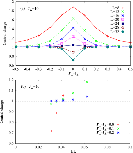
Figure 6: (Color Online) (a) Central charge of the $s=1/2$ three-leg spin tube  (1) with $J_{\perp}=10$, as functions of $J^{\prime}_{\perp}-J_{\perp}$. (b) System-size dependence of the central charge near the symmetric limit, as a function of $1/L$.

We study systems with $L=8$, $12$, $16$, $20$, $24$, $28$, and $32$ under the PBC, and keep $m\simeq 800$, $1400$, $2200$, $3000$, $4000$, $5000$, and $6000$ density-matrix eigenstates, respectively. An evaluation of the central charge with Eq. (51) needs extremely high accuracy of numerical data but gives a sharp insight for the thermodynamic limit even with small systems. The results for two strong rung-coupling cases $J_{\perp}=100$ and $J_{\perp}=10$ are shown in FIG. 5 and 6, respectively. At the symmetric point ($J^{\prime}_{\perp}=J_{\perp}$), the central charge deviates toward $c(L)\simeq 2$ for small $L$ because the system behaves as two decoupled spin and chirality chains from the viewpoint of RG; however apparently, it decreases with increasing $L$, cuts across $c=1$, and goes down to zero as approaching the thermodynamic limit. The similar behaviors are seen at $|J^{\prime}_{\perp}-J_{\perp}|=0.1$ for both of $J_{\perp}=100$ and $J_{\perp}=10$. The decay of $c(L)$ with decreasing $1/L$ is much slower than that at the symmetric point. However, it is natural to expect that it is extrapolated to zero in the thermodynamic limit once it comes down to $c<1$, since the existence of any nontrivial fixed point with $0<c<1$ is not expected. Therefore, the system is still in the dimer phase at $|J^{\prime}_{\perp}-J_{\perp}|=0.1$. On the other hand, $c(L)$ appears to converge to $1$ with decreasing $1/L$ at $|J^{\prime}_{\perp}-J_{\perp}|=0.2$. This means that the system behaves as a TLL at $|J^{\prime}_{\perp}-J_{\perp}|=0.2$, within the system sizes up to $L=32$ studied here. However, it should be noted that this does not exclude the possibility that the system is actually gapped in the thermodynamic limit but the correlation length is larger than $32$. Indeed, the exponentially large correlation length is expected in the gapped side of the BKT transition. Thus the present result does not contradict with the level spectroscopy analysis of the effective Hamiltonian in Sec. IV.1, that implies the critical point at $|J^{\prime}_{\perp}-J_{\perp}|\sim 0.283$.

Although a precise estimation of the BKT transition point is difficult in the present direct analysis due to the exponentially large correlation length and restriction of the system lengths, we can conclude that the dimer phase is extended to at least $|J^{\prime}_{\perp}-J_{\perp}|\leq 0.1$. This is indeed consistent with the level spectroscopy analysis of the effective Hamiltonian. As expected from the above theoretical and numerical analyses for the effective Hamiltonian (14), the BKT transition between the TLL and dimer phases occurs at a very small value of $|J^{\prime}_{\perp}-J_{\perp}|$ relative to $J_{\perp}$, in the strong rung-coupling regime.

V Conclusion

In this paper, we have discussed the quantum phase transitions of the three-leg spin tube induced by the modulation of the rung couplings. In the strong rung-coupling limit $J_{\perp}\gg J_{\parallel}$, the $s=$ half-odd-integer tube is mapped onto an effective model which is regarded as a special type of the spin-orbital models, where the orbital degrees of freedom correspond to the chirality ones in the original spin tube. The effective model was studied using the bosonization and RG techniques. For the symmetric tube ($J^{\prime}_{\perp}=J_{\perp}$), we found that the system is in the dimer phase with a finite excitation gap for the general spin-$s$ cases. Then, we investigated an effect of the asymmetric modulation of the rung couplings, which appears as a transverse chirality field in the effective Hamiltonian. For the asymmetric tube ($J^{\prime}_{\perp}\neq J_{\perp}$), we confirmed that the phase transition between the dimer and TLL phases is a BKT transition governed by the ordinary sine-Gordon model.

Furthermore, we performed the level spectroscopy analysis of the strong rung-coupling effective Hamiltonian using exact diagonalization and determine the BKT transition point to be $|J^{\prime}_{\perp}-J_{\perp}|=0.283$. Moreover, using the DMRG method we calculated the central charge of the original $s=1/2$ spin tube in the strong rung-coupling regime $J_{\perp}=10$ and $100$. Although the direct numerical analysis of the original spin tube model does not allow a precise determination of the transition point, we found that the dimer phase is robust against the modulation up to $|J^{\prime}_{\perp}-J_{\perp}|=0.1$, in agreement with the analysis based on the effective Hamiltonian. Thus, we conclude that the dimer phase persists for very small but a finite modulation of the rung couplings in the strong rung-coupling regime. It was also shown that the universal properties of the three-leg spin tube are essentially the same as those of the frustrated $J_{1}$-$J_{2}$ chain, as suggested in Ref. Sakai et al., 2008 and Sakai et al., 2010.

Our analyses are based on the strong rung-coupling expansion for $J_{\perp},J^{\prime}_{\perp}\gg J_{\parallel}$ and it is quite hard to speculate the low-energy properties in the intermediate and weak rung-coupling regimes. However, very recently, it was suggested that the BKT transition for the rung modulation occurs even in the weak rung-coupling regime with using the bosonization approach. Furuya and Oshikawa

*

Appendix A Strong rung-coupling Hamiltonian for general spin-$s$

In this appendix, we give a detailed derivation of the strong rung-coupling Hamiltonian (14) for general spin-$s$. For the angular momentum algebraic technique, see Ref. Edmonds, 1957.

We start with the construction of eigenstates with total spin $S$. For this purpose, ${\vec{s}}_{1}$ and ${\vec{s}}_{3}$ are first combined, and then ${\vec{s}}_{2}$ is added to ${\vec{S}}_{13}$:

$$\left|S_{13};SM\right> = \left|\left(\left(s_{3}s_{1}\right)S_{13}s_{2}\right)SM\right>$$

$$= \sum_{m_{1}m_{2}m_{3}}\left(sm_{3}sm_{1}|S_{13}\ m_{1}+m_{3}\right)$$

$$\times\left(S_{13}\ m_{1}+m_{3}\ sm_{2}|SM\right)\left|m_{1}m_{2}m_{3}\right>,$$

where the summation of $m_{j}$ runs over from $-s$ to $s$, and $\left(sms^{\prime}m^{\prime}|SM\right)$ is the Clebsch-Gordan coefficient. By applying the exchange operator ${\hat{P}}$ between ${\vec{s}}_{1}$ and ${\vec{s}}_{3}$ to Eq. (LABEL:eq:StateS13), we obtain

$${\hat{P}}\left|S_{13};SM\right> = \sum_{m_{1}m_{2}m_{3}}\left(sm_{3}sm_{1}|S_{13}\ m_{1}+m_{3}\right)$$ (53)

$$\times\left(S_{13}\ m_{1}+m_{3}\ sm_{2}|SM\right)\left|m_{3}m_{2}m_{1}\right>$$

$$= \left(-1\right)^{2s-S_{13}}\left|S_{13};SM\right>,$$

where $\left(sms^{\prime}m^{\prime}|SM\right)=\left(-1\right)^{s+s^{\prime}-S}\left(s^{\prime}m^{\prime}sm|SM\right)$ is used. Thus, $\left|S_{13};SM\right>$ is an eigenstate of ${\hat{P}}$. Here, we restrict the $S=1/2$ case, i.e., $S_{13}=s\pm 1/2$, and then the eigenstates of ${\hat{P}}$ are denoted as

$$\left|M+\right>\equiv\left|S_{13}=s+\frac{1}{2};S=\frac{1}{2},M\right>$$ (54)

for $P=\left(-1\right)^{s-1/2}$ and

$$\left|M-\right>\equiv\left|S_{13}=s-\frac{1}{2};S=\frac{1}{2},M\right>$$ (55)

for $P=\left(-1\right)^{s+1/2}$. These states are also eigenstates of the Hamiltonian (3) and their energy eigenvalues are given by Eq. (12).

For later convenience, we introduce an alternative expression of the eigenstate with $S$. Here, just as Eq.(LABEL:eq:StateS13) was obtained, we first combine ${\vec{s}}_{2}$ with ${\vec{s}}_{3}$ and then add ${\vec{s}}_{1}$ to ${\vec{S}}_{23}$. As a result, we have

$$\left|\left(s_{1}\left(s_{2}s_{3}\right)S_{23}\right)SM\right>$$ (56)

$$= \sum_{m_{1}m_{2}m_{3}}\left(sm_{2}sm_{3}|S_{23}\ m_{2}+m_{3}\right)$$

$$\times\left(sm_{1}S_{23}\ m_{2}+m_{3}|SM\right)\left|m_{1}m_{2}m_{3}\right>,$$

and this expression is related to Eq. (LABEL:eq:StateS13) by

$$\left<\left(s_{1}\left(s_{2}s_{3}\right)S_{23}\right)SM|S_{13};SM\right>$$ (59)

$$= \left(-1\right)^{3s+S_{23}-S_{13}+S}\sqrt{\left(2S_{13}+1\right)\left(2S_{23}+1\right)}\left\{\begin{array}[]{ccc}s&s&S_{23}\\ s&S&S_{13}\end{array}\right\},$$

where $\left\{\begin{array}[]{ccc}s_{1}&s_{2}&S_{12}\\ s_{3}&S&S_{13}\end{array}\right\}$ is the Wigner’s 6-j symbol. Therefore, we can write

$$\left|S_{13};SM\right>$$ (64)

$$= \sum_{S_{23}}\left(-1\right)^{3s+S_{23}-S_{13}+S}\sqrt{\left(2S_{13}+1\right)\left(2S_{23}+1\right)}$$

$$\times\left\{\begin{array}[]{ccc}s&s&S_{23}\\ s&S&S_{13}\end{array}\right\}\sum_{m_{1}m_{2}m_{3}}\left(sm_{2}sm_{3}|S_{23}\ m_{2}+m_{3}\right)$$

$$\times\left(sm_{1}S_{23}\ m_{2}+m_{3}|SM\right)\left|m_{1}m_{2}m_{3}\right>.$$

Now, our aim is to derive the strong rung-coupling Hamiltonian for $H=H_{0}+H_{1}$, where $H_{0}$ is the unperturbed part,

$$H_{0}=\sum_{i=1}^{L}\left[J_{\perp}\left({\vec{s}}_{i,1}\cdot{\vec{s}}_{i,2}+{\vec{s}}_{i,2}\cdot{\vec{s}}_{i,3}\right)+J^{\prime}_{\perp}{\vec{s}}_{i,1}\cdot{\vec{s}}_{i,3}\right],$$

(65)

and $H_{1}$ is the perturbation,

$$H_{1}=J_{\parallel}\sum_{i=1}^{L}\sum_{j=1}^{3}{\vec{s}}_{i+1,j}\cdot{\vec{s}}_{i,j}.$$ (66)

The projection operator onto the Hilbert space consisting of direct products of the $S=1/2$ states is defined as

$$Q=\prod_{i=1}^{L}Q_{i},\hskip 10.0ptQ_{i}=\sum_{M_{i}P_{i}}\left|M_{i}P_{i}\right>\left<M_{i}P_{i}\right|,$$ (67)

where $P_{i}$ takes the values $\pm 1$ corresponding to Eqs. (54) and (55). The strong rung-coupling Hamiltonian is then written as $H_{SC}=QHQ$. Using Eqs. (8) and (12), the unperturbed part $QH_{0}Q$ is easily calculated as

$$QH_{0}Q=\frac{2s+1}{2}\left(J^{\prime}_{\perp}-J_{\perp}\right)\sum_{i=1}^{L}\tau^{z}_{i}+{\rm const.}$$ (68)

In order to calculate the perturbation part $QH_{1}Q$, we consider the projected representation of $s_{i,j}^{\mu}$ ($\mu=x,y,z$),

$$Q_{i}s_{i,j}^{\mu}Q_{i} = \sum_{M_{i}M^{\prime}_{i}P_{i}P^{\prime}_{i}}\left|M_{i}P_{i}\right>\left<M_{i}P_{i}\right|s_{i,j}^{\mu}\left|M^{\prime}_{i}P^{\prime}_{i}\right>\left<M^{\prime}_{i}P^{\prime}_{i}\right|$$

$$= \sum_{M_{i}M^{\prime}_{i}P_{i}P^{\prime}_{i}}\zeta^{(j)}_{P_{i}P^{\prime}_{i}}\left|M_{i}\right>\left<M_{i}\right|S_{i}^{\mu}\left|M^{\prime}_{i}\right>\left<M^{\prime}_{i}\right|,$$

where we define

$$\zeta^{(j)}_{PP^{\prime}} \equiv \frac{\left<MP\right|s^{\mu}_{j}\left|M^{\prime}P^{\prime}\right>}{\left<M\right|S^{\mu}\left|M^{\prime}\right>}$$ (70)

$$= \frac{\left<M=\uparrow P||s_{j}||M^{\prime}=\uparrow P^{\prime}\right>}{\left<M=\uparrow||S||M^{\prime}=\uparrow\right>}$$

$$= 2\left<M=\uparrow P\right|s^{z}_{j}\left|M^{\prime}=\uparrow P^{\prime}\right>$$

and use the Wigner-Eckart theorem. The perturbation part is now expressed as

$$QH_{1}Q = J_{\parallel}\sum_{i=1}^{L}{\vec{S}}_{i}\cdot{\vec{S}}_{i+1}\sum_{P_{i}P_{i+1}P^{\prime}_{i}P^{\prime}_{i+1}}$$

$$\times\sum_{j=1}^{3}\zeta^{(j)}_{P_{i}P^{\prime}_{i}}\zeta^{(j)}_{P_{i+1}P^{\prime}_{i+1}}\left|P_{i}P_{i+1}\right>\left<P^{\prime}_{i}P^{\prime}_{i+1}\right|.$$

Using the parity operator ${\vec{\tau}}$ and the Hermiticity of the coefficient $\zeta^{(j)}_{PP^{\prime}}=\left(\zeta^{(j)}_{P^{\prime}P}\right)^{*}$, Eq. (LABEL:eq:QH1Q) is rewritten as

$$QH_{1}Q = J_{\parallel}\sum_{i=1}^{L}{\vec{S}}_{i}\cdot{\vec{S}}_{i+1}\sum_{j=1}^{3}[\frac{1}{2}(\zeta_{++}^{(j)}+\zeta_{--}^{(j)})+(\zeta_{++}^{(j)}-\zeta_{--}^{(j)})\tau_{i}^{z}+2\zeta_{+-}^{(j)}\tau_{i}^{x}]$$ (72)

$$\times[\frac{1}{2}(\zeta_{++}^{(j)}+\zeta_{--}^{(j)})+(\zeta_{++}^{(j)}-\zeta_{--}^{(j)})\tau_{i+1}^{z}+2\zeta_{+-}^{(j)}\tau_{i+1}^{x}].$$

From the exchange symmetry (${\vec{s}}_{1}\leftrightarrow{\vec{s}}_{3}$), the coefficient $\zeta^{(j)}_{PP^{\prime}}$ obeys

$$\zeta^{(1)}_{PP^{\prime}}=PP^{\prime}\zeta^{(3)}_{PP^{\prime}},\hskip 10.0pt\zeta^{(2)}_{PP^{\prime}}=\delta_{PP^{\prime}}\zeta^{(2)}_{PP}.$$ (73)

Here, the only thing we have to do is to evaluate the coefficient $\zeta^{(j)}_{PP^{\prime}}$. The calculation of $\zeta^{(2)}_{PP}$ may be relatively easy: It is given by

$$\zeta^{(2)}_{++} = 2\left<\uparrow+\right|s^{z}_{2}\left|\uparrow+\right>$$ (74)

$$= 2\sum_{m_{1}m_{2}m_{3}}m_{2}\left(sm_{3}sm_{1}|s+\frac{1}{2}\ m_{1}+m_{3}\right)^{2}\left(s+\frac{1}{2}\ m_{1}+m_{3}\ sm_{2}|\frac{1}{2}\frac{1}{2}\right)^{2}$$

$$= 2\sum_{m_{2}=-s}^{s}m_{2}\left(s+\frac{1}{2}\ \frac{1}{2}-m_{2}\ sm_{2}|\frac{1}{2}\frac{1}{2}\right)^{2}$$

$$= -\frac{2s}{3},$$

and

$$\zeta^{(2)}_{--} = 2\left<\uparrow-|s^{z}_{2}|\uparrow-\right>$$ (75)

$$= 2\sum_{m_{1}m_{2}m_{3}}m_{2}\left(sm_{3}sm_{1}|s-\frac{1}{2}\ m_{1}+m_{3}\right)^{2}\left(s-\frac{1}{2}\ m_{1}+m_{3}\ sm_{2}|\frac{1}{2}\frac{1}{2}\right)^{2}$$

$$= 2\sum_{m_{2}=-s+1}^{s}m_{2}\left(s-\frac{1}{2}\ \frac{1}{2}-m_{2}\ sm_{2}|\frac{1}{2}\frac{1}{2}\right)^{2}$$

$$= \frac{2\left(s+1\right)}{3},$$

where we use the unitarity of the Clebsch-Gordan coefficient, and the following formulas,

$$\left(s+\frac{1}{2}\ \frac{1}{2}-m\ sm|\frac{1}{2}\frac{1}{2}\right)^{2} = \frac{s-m+1}{(s+1)(2s+1)},$$

$$\left(s-\frac{1}{2}\ \frac{1}{2}-m\ sm|\frac{1}{2}\frac{1}{2}\right)^{2} = \frac{s+m}{s(2s+1)}.$$ (76)

It seems to be slightly more complicated to calculate $\zeta^{(1)}_{PP^{\prime}}$: Using the expression in Eq. (64), we obtain

$$\zeta^{(1)}_{++} = 2\left<\uparrow+\right|s^{z}_{1}\left|\uparrow+\right>$$ (82)

$$= 8\left(s+1\right)^{2}\left\{\begin{array}[]{ccc}s&s&s+\frac{1}{2}\\ s&\frac{1}{2}&s+\frac{1}{2}\end{array}\right\}^{2}\sum_{m_{1}=-s}^{s}m_{1}\left(s+\frac{1}{2}\ \frac{1}{2}-m_{1}\ sm_{1}|\frac{1}{2}\frac{1}{2}\right)^{2}$$

$$+8s\left(s+1\right)\left\{\begin{array}[]{ccc}s&s&s-\frac{1}{2}\\ s&\frac{1}{2}&s+\frac{1}{2}\end{array}\right\}^{2}\sum_{m_{1}=-s+1}^{s}m_{1}\left(s-\frac{1}{2}\ \frac{1}{2}-m_{1}\ sm_{1}|\frac{1}{2}\frac{1}{2}\right)^{2}$$

$$= \frac{2s+3}{6},$$ (83)

$$\zeta^{(1)}_{--} = 2\left<\uparrow-\right|s^{z}_{1}\left|\uparrow-\right>$$ (89)

$$= 8s\left(s+1\right)\left\{\begin{array}[]{ccc}s&s&s+\frac{1}{2}\\ s&\frac{1}{2}&s-\frac{1}{2}\end{array}\right\}^{2}\sum_{m_{1}=-s}^{s}\left(s+\frac{1}{2}\ \frac{1}{2}-m_{1}sm_{1}|\frac{1}{2}\frac{1}{2}\right)^{2}$$

$$+8s^{2}\left\{\begin{array}[]{ccc}s&s&s-\frac{1}{2}\\ s&\frac{1}{2}&s-\frac{1}{2}\end{array}\right\}^{2}\sum_{m_{1}=-s+1}^{s}m_{1}\left(s-\frac{1}{2}\ \frac{1}{2}-m_{1}\ sm_{1}|\frac{1}{2}\frac{1}{2}\right)^{2}$$

$$= \frac{-2s+1}{6},$$ (90)

and

$$\zeta^{(1)}_{+-} = 2\left<\uparrow+\right|s^{z}_{1}\left|\uparrow-\right>$$ (100)

$$= -8\sqrt{s(s+1)^{3}}\left\{\begin{array}[]{ccc}s&s&s+\frac{1}{2}\\ s&\frac{1}{2}&s+\frac{1}{2}\end{array}\right\}\left\{\begin{array}[]{ccc}s&s&s+\frac{1}{2}\\ s&\frac{1}{2}&s-\frac{1}{2}\end{array}\right\}\sum_{m_{1}=-s}^{s}m_{1}\left(s+\frac{1}{2}\ \frac{1}{2}-m_{1}\ sm_{1}|\frac{1}{2}\frac{1}{2}\right)^{2}$$

$$-8\sqrt{s^{3}(s+1)}\left\{\begin{array}[]{ccc}s&s&s-\frac{1}{2}\\ s&\frac{1}{2}&s+\frac{1}{2}\end{array}\right\}\left\{\begin{array}[]{ccc}s&s&s-\frac{1}{2}\\ s&\frac{1}{2}&s-\frac{1}{2}\end{array}\right\}\sum_{m_{1}=-s+1}^{s}m_{1}\left(s-\frac{1}{2}\ \frac{1}{2}-m_{1}\ sm_{1}|\frac{1}{2}\frac{1}{2}\right)^{2}$$

$$= \frac{2s+1}{2\sqrt{3}},$$ (101)

where we have used Eq. (76) and the following 6-j symbol formulas,

$$\left\{\begin{array}[]{ccc}s&s&s+\frac{1}{2}\\ s&\frac{1}{2}&s+\frac{1}{2}\end{array}\right\} = (-1)^{3s+1/2}\frac{1}{4(s+1)},$$ (104)

$$\left\{\begin{array}[]{ccc}s&s&s-\frac{1}{2}\\ s&\frac{1}{2}&s-\frac{1}{2}\end{array}\right\} = (-1)^{3s-1/2}\frac{1}{4s},$$ (107)

$$\left\{\begin{array}[]{ccc}s&s&s+\frac{1}{2}\\ s&\frac{1}{2}&s-\frac{1}{2}\end{array}\right\} = \left\{\begin{array}[]{ccc}s&s&s-\frac{1}{2}\\ s&\frac{1}{2}&s+\frac{1}{2}\end{array}\right\}$$ (112)

$$= (-1)^{3s+1/2}\frac{1}{4}\sqrt{\frac{3}{s(s+1)}}.$$ (113)

Substituting the above expressions of $\zeta^{(j)}_{PP^{\prime}}$ into Eq. (72), the perturbation part is obtained as

$$QH_{1}Q = \frac{J_{\parallel}}{3}\sum_{i=1}^{L}{\vec{S}}_{i}\cdot{\vec{S}}_{i+1}$$

$$\times\left[1+2(2s+1)^{2}\left(\tau^{x}_{i}\tau^{x}_{i+1}+\tau^{z}_{i}\tau^{z}_{i+1}\right)\right]$$

Incorporating Eqs. (68) and (LABEL:eq:QH1Q3) and applying an appropriate unitary transformation, we finally obtain the strong rung-coupling Hamiltonian (14).

References

- Gogolin et al. (1998) A. O. Gogolin, A. A. Nersesyan, and A. M. Tsvelik, Bosonization and Strongly Correlated Systems (Cambridge University Press, Cambridge, 1998).
- Giamarchi (2003) T. Giamarchi, Quantum Physics in One Dimension (Oxford University Press, New York, 2003).
- Haldane (1983) F. D. M. Haldane, Phys. Lett. A 93, 464 (1983).
- Sierra (1996) G. Sierra, J. Phys. A: Math. Gen. 29, 3299 (1996).
- Dell’Aringa et al. (1997) S. Dell’Aringa, E. Ercolessi, G. Morandi, P. Pieri, and M. Roncaglia, Phys. Rev. Lett. 78, 2457 (1997).
- White et al. (1994) S. R. White, R. M. Noack, and D. J. Scalapino, Phys. Rev. Lett. 73, 886 (1994).
- Reigrotzki et al. (1994) M. Reigrotzki, H. Tsunetsugu, and T. M. Rice, J. Phys.: Condens. Matter 6, 9235 (1994).
- Hatano and Nishiyama (1995) N. Hatano and Y. Nishiyama, J. Phys. A: Math. Gen. 28, 3911 (1995).
- Greven et al. (1996) M. Greven, R. J. Birgeneau, and U. J. Wiese, Phys. Rev. Lett. 77, 1865 (1996).
- Totsuka and Suzuki (1996) K. Totsuka and M. Suzuki, J. Phys. A: Math. Gen. 29, 3559 (1996).
- Schulz (1996) H. J. Schulz, in Correlated Fermions and Transport in Mesoscopic Systems, edited by T. Martin, G. Montambaux, and J. Trân Thanh Vân (Editions Frontières, Gif-sur-Yvette, 1996) p. 81, see also e-print \htmladdnormallinkarXiv:condmat/9605075http://arxiv.org/abs/cond-mat/9605075.
- Kawano and Takahashi (1997) K. Kawano and M. Takahashi, J. Phys. Soc. Jpn. 66, 4001 (1997).
- Cabra et al. (1997) D. C. Cabra, A. Honecker, and P. Pujol, Phys. Rev. Lett. 79, 5126 (1997).
- Cabra et al. (1998) D. C. Cabra, A. Honecker, and P. Pujol, Phys. Rev. B 58, 6241 (1998).
- Orignac et al. (2000) E. Orignac, R. Citro, and N. Andrei, Phys. Rev. B 61, 11533 (2000).
- Lüscher et al. (2004) A. Lüscher, R. M. Noack, G. Misguich, V. N. Kotov, and F. Mila, Phys. Rev. B 70, 060405 (2004).
- Nishimoto and Arikawa (2008) S. Nishimoto and M. Arikawa, Phys. Rev. B 78, 054421 (2008).
- Sakai et al. (2008) T. Sakai, M. Sato, K. Okunishi, Y. Otsuka, K. Okamoto, and C. Itoi, Phys. Rev. B 78, 184415 (2008).
- Sakai et al. (2010) T. Sakai, M. Sato, K. Okamoto, K. Okunishi, and C. Itoi, J. Phys.: Condens. Matter 22, 403201 (2010).
- Sakai et al. (2005) T. Sakai, M. Matsumoto, K. Okunishi, K. Okamoto, and M. Sato, Physica E 29, 633 (2005).
- Charrier et al. (2010) D. Charrier, S. Capponi, M. Oshikawa, and P. Pujol, Phys. Rev. B 82, 075108 (2010).
- Haldane (1982a) F. D. M. Haldane, Phys. Rev. B 25, 4925 (1982a).
- Haldane (1982b) F. D. M. Haldane, Phys. Rev. B 26, 5257 (1982b).
- Okamoto and Nomura (1992) K. Okamoto and K. Nomura, Phys. Lett. A 169, 433 (1992).
- Li et al. (2013) W. Li, A. Weichselbaum, and J. von Delft, Phys. Rev. B 88, 245121 (2013).
- Plat et al. (2012) X. Plat, S. Capponi, and P. Pujol, Phys. Rev. B 85, 174423 (2012).
- Nishimoto et al. (2011) S. Nishimoto, Y. Fuji, and Y. Ohta, Phys. Rev. B 83, 224425 (2011).
- Schnack et al. (2004) J. Schnack, H. Nojiri, P. Kögerler, G. J. T. Cooper, and L. Cronin, Phys. Rev. B 70, 174420 (2004).
- Fouet et al. (2006) J.-B. Fouet, A. Läuchli, S. Pilgram, R. M. Noack, and F. Mila, Phys. Rev. B 73, 014409 (2006).
- Kugel and Khomskii (1982) K. I. Kugel and D. I. Khomskii, Usp. Fiz. Nauk 136, 621 (1982), [Sov. Phys. Usp. 25, 231 (1982)].
- Pati and Singh (2000) S. K. Pati and R. R. P. Singh, Phys. Rev. B 61, 5868 (2000).
- Kolezhuk et al. (2001) A. K. Kolezhuk, H.-J. Mikeska, and U. Schollwöck, Phys. Rev. B 63, 064418 (2001).
- Note (1) In Ref. \rev@citealpnumPati00, although they only considered Eq. (16\@@italiccorr) in the regime, a canonical transformation makes a change and . Thus, their model still includes the effective Hamiltonian (14\@@italiccorr) with and .
- Nishimoto and Arikawa (2010) S. Nishimoto and M. Arikawa, J. Phys.: Conf. Ser. 200, 022039 (2010).
- Lukyanov (1998) S. Lukyanov, Nucl. Phys. B 522, 533 (1998).
- Hikihara and Furusaki (1998) T. Hikihara and A. Furusaki, Phys. Rev. B 58, R583 (1998).
- Takayoshi and Sato (2010) S. Takayoshi and M. Sato, Phys. Rev. B 82, 214420 (2010).
- Orignac (2004) E. Orignac, Eur. Phys. J. B 39, 335 (2004).
- Orignac and Giamarchi (1998) E. Orignac and T. Giamarchi, Phys. Rev. B 57, 5812 (1998).
- Cardy (1996) J. Cardy, Scaling and Renormalization Group in Statistical Physics (Cambridge University Press, Cambridge, 1996).
- Kim and Sólyom (1999) E. H. Kim and J. Sólyom, Phys. Rev. B 60, 15230 (1999).
- Affleck et al. (1989) I. Affleck, D. Gepner, H. J. Schulz, and T. Ziman, J. Phys. A: Math. Gen. 22, 511 (1989).
- Cardy (1984) J. L. Cardy, J. Phys. A: Math. Gen. 17, L385 (1984).
- Ziman and Schulz (1987) T. Ziman and H. J. Schulz, Phys. Rev. Lett. 59, 140 (1987).
- Cardy (1986a) J. L. Cardy, Nucl. Phys. B 270, 186 (1986a).
- Cardy (1986b) J. L. Cardy, J. Phys. A: Math. Gen. 19, L1093 (1986b).
- White (1992) S. R. White, Phys. Rev. Lett. 69, 2863 (1992).
- Schollwöck (2005) U. Schollwöck, Rev. Mod. Phys. 77, 259 (2005).
- Calabrese and Cardy (2004) P. Calabrese and J. Cardy, J. Stat. Mech. 2004, P06002 (2004).
- Nishimoto (2011) S. Nishimoto, Phys. Rev. B 84, 195108 (2011).
- (51) S. C. Furuya and M. Oshikawa, unpublished.
- Edmonds (1957) A. R. Edmonds, Angular Momentum in Quantum Mechanics (Princeton University Press, New Jersey, 1957).