On the spectral origin of non-Markovianity: an exact finite model

Abstract

Non-homogeneous chain environments (e.g. segmented ion traps) are investigated through an exact diagonalization approach. Different spectral densities, including band-gaps, can be engineered to separately assess memory effects. Environment non-Markovianity is quantified with recently introduced measures of information flow-back and non-divisibility of the system dynamical map. By sweeping the bath spectrum via tuning of the system frequency we show strongest memory effect at band-gap edges and provide an interpretation based on energy flow between system and environment. A system weakly coupled to a stiff chain ensures a Markovian dynamics, while the size of the environment as well as the local density of modes are not substantial factors. We show an opposite effect when increasing the temperature inside or outside the spectral band-gap. Further, non-Markovianity arises for larger (negative and positive) powers of algebraic spectral densities, being the Ohmic case not always the most Markovian one.

Introduction. Achievements in preparation, control and measurements of quantum systems require a deep understanding of the mechanism of interaction between a given open quantum system and the surrounding environment WeiBreGar . From a theoretical point of view, popular approaches, e.g. derivations of master or quantum Langevin equations WeiBreGar ; Hanggi , are based on the assumption of an infinite heat bath with some given spectral density $J(\omega)$ embedding all information about the real couplings and frequencies in the complex environment, and the structure of the coupling to the system. Typical approximations to simplify the treatment, such as negligible memory effects (Markovian approximation), system time coarse graining, weak system-bath coupling, large frequency cut-off, Ohmic spectral density, drastically constrain the possible frequency dependence of $J(\omega)$. Although simplified spectral densities allow an analytical treatment, important deviations from these simple instances are common in several systems like, for instance, electric circuits, acoustic polarons in metals and semi-conductors, radiation damping of charged particles WeiBreGar , photonic crystals John ; TanZha ; PriPle ; Hoeppe , but also in ion traps suffering electric field noise Hite , micro-mechanical oscillators aspelmeyerEisert or polarized photons for broad frequency spectra EXP_opt_NM .

Memory effects and deviations from Markovian dynamics have been widely explored considering the time dependence of master equation-coefficients and deviations from exponential decays WeiBreGar ; Haake ; HPZ ; nori but only in the last few years several approaches have been proposed to systematically distinguish Markovian evolution in terms of properties of the dynamical map NM1 ; BLP ; RHP ; local_NM . Different measures allow to quantify non-Markovianity (NM) in terms of deviations from the Lindblad form of the generator of the master equation NM1 , flow-back of information from the environment BLP , and entanglement decay with an ancilla RHP , to mention some of them. The recent endeavor to better characterize memory effects in open systems not only aims to a deeper understanding of dissipative dynamics in physical, biological and chemical systems, but is also explored as a resource in quantum technologies NMappl .

The aim of this work is to identify non-Markovian effects originating in the structure of the system and bath couplings as well as in the distribution of energies, as given by the form of the spectral density $J(\omega)$. To this end we consider a microscopic model given by an inhomogeneous harmonic chain, avoiding the limitations of approximate approaches. Finite models of coupled oscillators have been used to assess entanglement dynamics PleEis and its generation when attaching ions to a chain Morigi1 and can also provide an insightful test-bed to establish the regimes of validity of approximated master equations RivPle . The case of an oscillator attached to a homogeneous chain was already studied by Rubin to determine the statistical properties of crystals with defects: this configuration leads to a Ohmic dissipation (thus Markovian, at least for large temperature) rubin . Moving to non-homogeneous chain configurations, we inquire the origin of NM to distinguish among several independent features quantifying separately different sources of NM. When focusing on periodic systems (e.g. dimers), we can engineer spectral densities with finite band-gaps, like in semiconductors or photonic crystals AshMer ; John ; TanZha ; PriPle . For suitable couplings we show that the system is actually influenced by the resonant portion of the environment. Memory effects BLP ; RHP are then evaluated by sweeping the spectral density for a structured bath allowing us to show the effects of the local form of the spectrum.

Before introducing the model, we point out that experimental implementation of a tunable chain of oscillators can be obtained through recent progress in segmented Paul traps Kaler ; Wineland also allowing tunability of ions couplings and onsite potentials. Other possible setups are based on photonic crystal nanocavities, microtoroid resonators (see hartmann for a review) or optomechanic resonators aspelmeyerEXP . Furthermore, correlations spectra of the system can be measured to gain insight on the spectral density induced by the rest of the chain (see aspelmeyerEisert ; nori ). The non-homogeneous harmonic chain we consider in this work represents then a structured and controllable reservoir amenable to experimental realization.

The system: non-homogeneous chain. We consider an open quantum system consisting of an harmonic oscillator $H_{S}=(p^{2}_{S}+\omega_{S}^{2}q^{2}_{S})/2$, where $p_{S}$ and $q_{S}$ are the system momentum and position operators, interacting with an environment ($E$) that consists of an harmonic chain of $N$ elements interacting through a spring-like coupling non-homogeneous along the chain. A particularly dramatic deviation from the Ohmic spectrum obtained with a homogeneous chain (Rubin model rubin ) is found when considering a periodic configuration (dimer) of identical oscillators with alternate values of couplings $g$ and $h\leq g$ (see Fig. 1)

$$H_{E}=\sum_{i}\bigl{(}p_{i}^{2}+\Omega_{i}^{2}q_{i}^{2}\bigl{)}/2-g\sum_{i}^{odd}q_{i}q_{i+1}-h\sum_{i}^{even}q_{i}q_{i+1}$$ (1)

with $\Omega_{i}=\sqrt{\omega_{0}^{2}+h+g}$ ($i=2...N-1$) and $\Omega_{1}=\Omega_{N}=\sqrt{\omega_{0}^{2}+g}$ footnote1 . For any $\omega_{0}$ and $g\neq h$ we build a band gap model, characterized by a frequency spectrum distributed in an acoustic and an optical band separated by a finite gap AshMer .

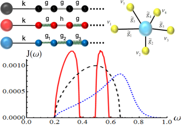
Figure 1: (Colors online) Examples of spectral densities which can be generated in our model: Rubin chain with $g=h=0.1$ and $k=0.01$ (black line), gapped spectral density with $g=0.1$, $h=0.05$ and $k=0.0075$ (red line), and increasing coupling density with $g_{i}=0.1+0.05\cdot i$ and $k=0.01$ (blue line). Bath frequency $\omega_{0}=0.2$ (in unspecified, but fixed, frequency units) in all examples. Schematic for the three plotted examples in the corresponding colors (top left) and of a star configuration (top right) also represented.

The system is attached to the first element of the E chain and $k$ is a coupling constant with an interaction term of the form $H_{I}=-kq_{S}q_{1}$. We consider an initial factorized state between system squeezed vacuum and a thermal bath at temperature $T$. The chain configuration for real oscillators is mapped by diagonalization of the environment (through an orthogonal transformation $\mathbf{K}$) into a star configuration of independent oscillators (bath’s eigenmodes) of frequency $\nu_{i}$ interacting with the system with strength $\tilde{g}_{i}=k\mathbf{K}_{1i}$ (see Fig. 1 and SupMat ).

Generalized Langevin equation. The reduced dynamics of the system is governed by a Langevin equation, typically derived starting from a star environment WeiBreGar ; Hanggi ,

$$\ddot{q}_{S}+\tilde{\omega}_{s}^{2}q_{S}+\int_{0}^{t}ds\gamma(t-s)\dot{q}_{S}={\xi}(t),$$ (2)

where ${\xi}(t)$ is Langevin forcing of the system LangFor and $\gamma(t)=\sum_{i}\bigl{(}\tilde{g}_{i}^{2}/\nu_{i}^{2}\bigl{)}\cos\bigl{(}\nu_{i}t\bigl{)}$ is the damping kernel accounting for dissipation and memory effects. The spectral density can be obtained from the damping kernel as $J(\omega)=\omega\int_{0}^{\infty}\gamma(t)\cos(\omega t)dt$. For a finite number $N$ of normal modes, the dissipative dynamics suffers recurrence for times $\tau_{R}$ (related to reflection into the system of the fastest signals traveling along the chain), whose value depends on the number of modes $N$ and on the frequency spectrum Estim . If we look at times $t<\tau_{R}$ the spectral density can be described by a smooth function of frequency. The form of this function can be directly related to the dynamical properties of the system. For instance, a linear –Ohmic– spectral density , i.e. $J(\omega)\propto\omega$, leads to a Markovian equation with time-independent friction kernel $-\gamma_{0}\dot{q}(t)$. In the Rubin model it is possible to show that $J(\omega)\propto\sqrt{\omega^{2}-\omega_{0}^{2}}\sqrt{\omega_{c}^{2}-\omega_{S}^{2}}\,\theta(\omega_{c}-\omega)$ with $\omega_{c}=\sqrt{2g}$ the highest (cutoff) frequency in the spectrum of normal modes. Other non-homogeneous chain examples are shown in Fig. 1.

Resonance conditions. In order to investigate the role of the spectral density’s shape, we first need to know to what extent the system is affected by different bath eigenmodes depending on their relative detuning. To do so we compare

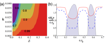
Figure 2: (Colors online) (a) Averaged fidelity as a function of system-bath coupling $k$ and bandwidth $\delta$, for a band gap density with $g=0.1$, $h=0.05$ and $\omega_{0}=0.3$ at temperature $T=0$. Integration performed up to $t_{F}=400$ for $N=50$ oscillators. (b) System excitation number at $t=400$ as a function of the proper frequency $\omega_{S}$ for a band gap model with $g=0.1$, $h=0.05$ and $\omega_{0}=0.3$ ($J(\omega)$ as shaded area) at $T=0$. System-bath coupling $k=0.005$ (red solid) and $k=0.025$ (blue dashed).

the state of the system $\rho(t)$ with $\rho_{\delta}(t)$ obtained by allowing the system to interact only with those normal modes whose frequencies lie within a range $\delta$ to system frequency $\omega_{S}$, i.e. such that $|\nu_{i}-\omega_{S}|<\delta$. The time evolution is obtained by a full diagonalization of $H_{S}+H_{R}+H_{I}$ SupMat . Deviation between $\rho(t)$ and $\rho_{\delta}(t)$ can be witnessed by the Uhlmann fidelity measure ZukBen , $\mathbf{F}(\rho,\rho_{\delta})=Tr\sqrt{\sqrt{\rho}\rho_{\delta}\sqrt{\rho}}$. This quantity averaged in time, $\int_{0}^{t_{F}}\mathbf{F}(\rho,\rho_{\delta})dt/t_{F}$, is shown in Fig. 2a for a band gap model with system frequency larger than the optical band, $\omega_{S}>\omega_{c}$. Here and in the following we choose $t_{F}<\tau_{R}$ but big enough to explore the dissipative dynamics. If we take the value $0.99$ as a guide for the eye, a weakly coupled oscillator ($k<0.01$) interacts only with a small vicinity of modes in the nearest band (right/optical band in Fig. 1), while already for $k=0.012$ we need to take into account modes in the furthest band (left/acoustic band). This rough estimation allows to appreciate that for weak couplings $k\ll\omega_{c}$ a reduced number of resonant bath modes suffice to determine the system evolution.

The effect of the environment band-gap is clearly shown by looking at the system excitation (average energy normalized by its frequency) $\langle H_{S}(\tau_{F})\rangle/\omega_{S}$ at $\tau_{F}$ by varying the system frequency $\omega_{S}$ to sweep the spectral density (Fig. 2b). Energy is dissipated continuously when $\omega_{S}$ is resonant with the bath while it can not propagate into the chain for $\omega_{S}$ within the band-gap (leading to oscillatory behavior and the formation of bound dressed states) AshMer ; John ; TanZha ; wang .

Non-Markovian dynamics. Among the different quantifiers of NM appeared recently in the literature we consider hereafter the Breuer-Laine-Piilo (BLP) BLP and Rivas-Huelga-Plenio (RHP) RHP measures. The first (BLP) gives an interpretation of NM in terms of a back-flow of information from the environment into the system. Its definition exploits the contractivity property of the quantum trace distance $\mathbf{D}$ under completely positive and trace preserving maps BLP . For continuous variable systems, and within Gaussian states, the definition has been extended by substituting the trace distance with the fidelity $\mathbf{F}$ VasGauNM ; IncFid , and the associated measure for the degree of NM reads

$$\mathbf{M}_{BLP}=\max_{\rho_{1},\rho_{2}}\int_{dF/dt<0}\frac{dF(\rho_{1},\rho_{2})}{dt}dt$$ (3)

where the maximization is taken among all pairs of Gaussian states $(\rho_{1},\rho_{2})$ and integration is performed up to $t_{F}$.

The RHP criterion witnesses the non-divisibility of the dynamical map by preparing the system in an entangled state with an ancilla and evaluating the non-monotonic time evolution of the entanglement. The measure reads RHP

$$\mathbf{M}_{RHP}=\int_{0}^{\tau_{R}}\biggl{|}\frac{dE_{SA}}{dt}\biggl{|}dt-E_{SA}(\tau_{R})+E_{SA}(0)$$ (4)

where $E_{SA}(t)$ denotes a proper system-ancilla entanglement measure, such as logarithmic negativity. We should stress that when Eq. (4) gives zero, the map can be either divisible or non-divisible. For details on the numerical evaluation of these measures see SupMat .

In Fig. 3 we show both NM measures for a dimer chain environment as a function of the system frequency $\omega_{S}$ for temperature $T=0$. We find that local NM maxima are present at the edges of the band-gap spectral density for both measures, while rapidly decreasing both inside the band and the gaps of the spectral density. Sharp changes in frequency lead to long times in the Fourier transform, and are responsible for broad noise and dissipation kernels, for long time bath correlations WeiBreGar ; RivPle and for pronounced NM signatures, Fig. 3. Full Markovian behavior is achieved only inside the band where $\mathbf{M}_{BLP}\sim 0$. Even if the null value of the RHP measure is inconclusive, we mention that increasing the system-bath coupling $k$, it raises to finite values, yielding a shape very much in agreement with the BLP measure. This is one the few comparisons of two different NM measures in the literature compare .

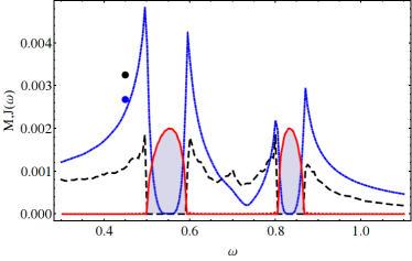
Figure 3: (color online) BLP non-Markovianity (blue) and RHP (black,dashed) for N=40 oscillators, $g=0.2$, $h=0.05$, $k=0.001$, $\omega_{0}=0.5$ as a function of $\omega_{S}$, for $T=0$. The red (continuous) curve represents the spectral density used in arbitrary units. The extra dots are evaluated at $\omega_{s}=0.45$ increasing the two-mode squeezing parameter from $r=1$ to $1.5$ (for RHP NM) and increasing the squeezing parameter range for the BLP NM maximization (from $r\in\{0.5,1\}$ to $r\in\{0.125,1.125\}$) SupMat .

We also notice that in correspondence with the edges of the spectral density $J(\omega)$, where $\mathbf{M}_{BLP}$ is larger, we find a higher density of modes. To exclude its connection with NM effects, we artificially engineered the spectral density to obtain a constant density of modes throughout the spectrum. This allows us to establish that the enhancement of NM at the edges is actually not related to the normal mode density of states. The origin of NM is elsewhere.

Interaction between system and environment ($H_{I}$) leads to energy exchange. When the system is in resonance with a band of the spectral density (optical or acoustical), energy is exchanged with many normal modes. In the real chain picture this corresponds to energy allowed to travel along the chain. This leads to an ever increasing indistinguishability of the states in Eq. 3 (all loosing energy and relaxing) and thus to a low value of NM. On the other hand, at the band edges and in the band-gaps, the energy lost by the system cannot travel freely along the chain, but bounces back and forth from the first elements of the chain to the system. This implies a periodical increase/decrease of distinguishability of the states whose fidelity we are integrating, hence we witness a higher NM value. The higher the detuning (deeper in the band-gap), the less excitations/energy are exchanged, resulting in a diminishing value for the BLP NM. This result is in accordance with Ref. nori , where they study a generic bosonic/fermionic reservoir, and show that band-gaps generate localized modes (thus dissipationless oscillatory behavior) plus nonexponential decays (identified there with NM). According to Ref. BLP , Fig. 3 provides a quantitative measure of NM at band-gap edges as flow back of information.

What makes a bath Markovian? Besides the resonance conditions and the back reflection of information/energy when the system is out of resonance with the bath, what are the main factors leading to more Markovian dynamics? We have tried to answer this question in a fivefold approach, namely, with respect to the bath’s size, its temperature, the width of its spectral density, its shape (sub-Ohmic, Ohmic, super-Ohmic) and the strength of its coupling to the system.

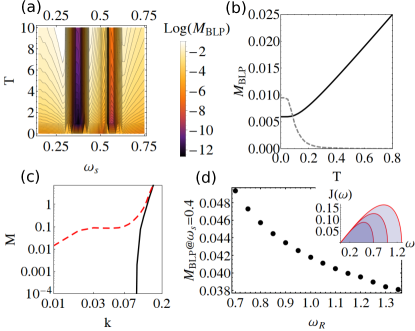
Figure 4: (color online) (a) log$(M_{BLP})$ for 50 oscillators, $g=0.1$, $h=0.05$, $k=0.001$ and $\omega_{0}=0.3$, for temperatures $T\in[0,10]$ and $\omega_{s}$ (the limits of the acoustic and optical bands are obvious from the discontinuity of $M_{BLP}$). (b) Temperature dependence of $M_{BLP}$ for $\omega_{s}=0.25~{}(0.375)$ in black (gray). (c) $M_{BLP}$ (dashed) and $M_{RHP}$ (continuous) at $\omega_{s}=0.575$ for an homogeneous 50 oscillators chain, $g=h=0.1$ and $\omega_{0}=0.3$. (d) No-gap (star-configuration) spectrum $J(\omega)=k\omega\sqrt{\omega_{R}^{2}-\omega^{2}}/\omega_{R}$ with 40 oscillators, $k=0.00001$, $\omega_{s}=0.4$ and varying $\omega_{R}$. (Inset shows $J(\omega)$ for three values of $\omega_{R}$.)

It is known that at low temperatures, Markovian approximations are generally not valid WeiBreGar and non-exponential decays of the correlation functions do arise Haake . In Fig. 4a we show that the back-flow of information $M_{BLP}$ is similarly present only at low temperatures ($T\lesssim\omega_{c}$) when the system is dissipating within a band of the spectral density. Surprisingly, when we move to a non-resonant configuration, with the frequency of the system in the band-gap, NM is found to increase with temperature, Fig. 4b. When increasing temperature to higher values a linear increase of NM is observed within the gap, while in the band $M_{BLP}$ tends to vanish.

Most prominent NM effects are expected in the strong coupling regime between system and bath WeiBreGar ; Haake : indeed reduction to Markovian dynamics is provided by a decrease of the coupling, which reduces NM by two orders of magnitude by one order of magnitude decrease in coupling. For the $M_{RHP}$ we see that it tends to zero very fast (remember that a zero value is inconclusive) Fig. 4c. The importance of frequency cut-off in the spectral density is relevant not only to avoid unphysical divergences but also when discussing NM in terms of relevant time scales. Interestingly, a chain environment allows to engineer the value of the frequency cut-off of an Ohmic environment by increasing the coupling strengths within the chain. As shown in Fig. 4d an increase of the width of the spectrum (stiff chains) allows for a monotonic flow of information into the environment leading to a decrease of NM. We also checked the dependence of NM with the bath size, seeing none (except for the role of the recurrence time).

Finally we built an artificial star model (Fig. 1) with equally spaced frequencies and couplings $\tilde{g}_{i}$ in order to isolate the effects of different algebraic behavior of the spectrum, looking, as common in the literature, at deviations from the Ohmic case. In Fig. 5 we show $M_{BLP}$ for algebraic spectral densities $J(\omega)\sim\omega^{s}$ with fixed sharp cutoffs at $0.25,0.75$. We consider both positive and negative algebraic forms aspelmeyerEisert and observe an increase of NM in both cases when departing from $s_{\rm min}\sim 1/2,1,1.4,2,2.8$ at temperatures $T=0,0.25,0.5,1,2$ ($T=2$ not shown).

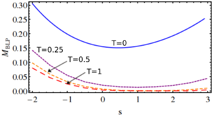
Figure 5: $M_{BLP}$ for the star-configuration density $J(\omega)=k(\omega/\omega_{S})^{s}\Theta(\omega-0.25)\Theta(0.75-\omega)$ ($\Theta$ is the step function) as a function of $s$ at $\omega_{s}=0.5$, for temperatures $T=0,0.25,0.5,1$.

Surprisingly, the lowest NM is achieved for $s=1/2$ at zero temperature, instead of $s=1$ (Ohmic case). For higher temperatures the lowest value is achieved for $s=1$ or a bit higher. Also, a bath with $J(\omega)\sim 1/\omega^{2}$ is more non-Markovian than one with $J(\omega)\sim\omega^{2}$. We also stress that different scaling and constraints of power functions densities lead to significant influence on memory effects SupMat .

Summary and conclusions.

We have considered different (non-phenomenological) spectral densities attainable by tuning non-homogeneous oscillators chains that can be implemented in segmented ion chains traps and also with nano-oscillators. A system attached at one extreme of the chain dissipates in this finite bath and exhibits memory effects. The importance of our analysis is the separate assessment, without approximations, of environment features that can be microscopically engineered and the quantitative comparison of two NM measures BLP ; RHP to establish their influence in retaining environment memory effects.

The possibility to tune the chain in a dimer configuration allows us to assess the influence of band-gaps and to obtain a more detailed picture on the origin of Markovianity in relation to specific features of the spectral density. The main role describing the behavior of NM is played by a resonance condition: if the system is resonant with the normal modes of the bath, energy transfer along the chain is allowed and therefore information and energy flow irreversibly from system to bath leading to a Markovian dynamics. The largest flow back of information is found at the edges of the gaps where the energy bounces between the system and bath.

A high frequency cutoff and weak coupling, the first obtained by increasing the stiffness of the chain and the latter by decreasing the system-bath coupling, are major factors for ensuring Markovian dynamics. Indeed, NM effect of strong coupling or frequency cut-off, have already been discussed in the literature and we find consistent results. A relevant point when dealing with finite systems is that actually neither the size of the bath is important (only matters in limiting the recurrence time) nor the local density of modes has any significant influence on memory effects.

On the other hand, unexpected results have been found when increasing temperature leading to opposite behavior inside and outside the band with a (linear in T) NM increase in the band-gap while inside the band memory effects become negligible for temperatures larger than the environment frequencies. Finally we have quantified NM when departing from the Ohmic case, considering positive and negative algebraic spectral densities $J(\omega)\propto\omega^{s}$ for $-2\leq s\leq 3$ (being $s=-2$ a recently measured value aspelmeyerEisert ) showing an enhancement of memory effects for both positive and negative values of $s$, with the Ohmic case (s=1) not being necessarily the most Markovian one.

I Supplementary information

Environmental diagonalization

Let’s consider the Hamiltonian $H_{E}$ and rewrite it in the following way

$$H_{E}=\frac{\mathbf{p}^{T}\mathbf{p}}{2}+\mathbf{q}^{T}\mathbf{A}\mathbf{q}$$ (5)

where we compact the position and momentum operators in a vector formalism, i.e. $\mathbf{q}\equiv\{q_{1},q_{2}...,q_{N}\}^{T}$ and $\mathbf{p}\equiv\{p_{1},p_{2}...,p_{N}\}^{T}$. Moreover we have an $N\times N$ matrix $\mathbf{A}$ with elements $\mathbf{A}_{ij}=\Omega_{i}^{2}\delta_{ij}/2-\mathbf{G}_{ij}/2$, where the connection matrix $\mathbf{G}$ has the following form

$$\mathbf{G}=\left(\begin{array}[]{cccccc}0&g&0&0&...&0\\ g&0&h&0&...&0\\ 0&h&0&g&...&0\\ 0&0&g&...&...&...\\ ...&...&...&...&0&g\\ 0&0&0&...&g&0\\ \end{array}\right)$$ (6)

Since $\mathbf{A}$ is symmetric, it can be diagonalized by an orthogonal transformation $\mathbf{K}$, i.e. $\mathbf{K}^{T}\mathbf{A}\mathbf{K}=\mathbf{D}$ where $\mathbf{D}$ is a the diagonal matrix containing the eigenvalues $\lambda_{i}$ of $\mathbf{A}$. Thus defining the new variables $\mathbf{Q}=\mathbf{K}^{T}\mathbf{q}$ and $\mathbf{P}=\mathbf{K}^{T}\mathbf{p}$, we can rewrite the hamiltonian as

$$H_{E}=\sum_{i=1}^{N}\biggl{[}\frac{P_{i}^{2}}{2}+\frac{\nu_{i}^{2}Q_{i}^{2}}{2}\biggl{]}$$ (7)

where the eigenfrequencies are $\nu_{i}=\sqrt{2\lambda_{i}}$,and again $\mathbf{Q}\equiv\{Q_{1},Q_{2}...,Q_{N}\}^{T}$ and $\mathbf{P}\equiv\{P_{1},P_{2}...,P_{N}\}^{T}$. Thus we passed from a chain environment into the equivalent star model.

Full Diagonalization and time evolution

The starting point is the total Hamiltonian $H=H_{S}+H_{E}+H_{I}$ after the diagonalization of the environment. Since $H$ is also quadratic in position and momentum operators, it can again be written as

$$H=\frac{\mathbf{p}^{T}\mathbf{p}}{2}+\mathbf{q}^{T}\mathbf{B}\mathbf{q}$$ (8)

where, contrary to the notation of last section, we have $\mathbf{q}\equiv\{q_{1},q_{2}...,q_{N},q_{S}\}^{T}$ and $\mathbf{p}\equiv\{p_{1},p_{2}...,p_{N},p_{S}\}^{T}$. The $(N+1)\times(N+1)$ matrix $\mathbf{B}$ has elements $\mathbf{B}_{ii}=\nu_{i}^{2}/2$ for $i=1....N$, $\mathbf{B}_{N+1N+1}=\omega_{S}^{2}/2$ and $\mathbf{B}_{i,N+1}=\mathbf{B}_{N+1,i}=-\tilde{g}_{i}/2$.

We can again perform a diagonalization of $\mathbf{B}$ through an orthogonal matrix $\mathbf{O}$, i.e. $\mathbf{O}^{T}\mathbf{B}\mathbf{O}=\mathbf{F}$, and upon defining the new system-environment normal modes $\mathbf{Q}=\mathbf{O}^{T}\mathbf{q}$ and $\mathbf{P}=\mathbf{O}^{T}\mathbf{p}$, we rewrite the full Hamiltonian as

$$H=\sum_{i=1}^{N+1}\biggl{[}\frac{P_{i}^{2}}{2}+\frac{f_{i}^{2}Q_{i}^{2}}{2}\biggl{]}$$ (9)

where $\sqrt{2f_{i}}$ are the eigenvalues of $\mathbf{B}$ contained in the diagonal matrix $\mathbf{F}$.

In this picture, the time evolution for each normal mode is trivial,

$$\begin{split}&Q_{i}(t)=Q_{i}(0)\cos\bigl{(}f_{i}t\bigl{)}+\frac{P_{i}(0)}{f_{i}}\sin\bigl{(}f_{i}t\bigl{)}\\ &P_{i}(t)=-f_{i}Q_{i}(0)\sin\bigl{(}f_{i}t\bigl{)}+P_{i}(0)\cos\bigl{(}f_{i}t\bigl{)}\end{split}$$ (10)

Now, remembering the new variables are connected to the old ones through the orthogonal transformation $\mathbf{O}$ at any time $t$, we easily get

$$\begin{split}&q_{i}(t)=\sum_{j=1}^{N+1}\bigl{[}\mathbf{B}^{QQ}_{ij}(t)q_{j}(0)+\mathbf{B}^{QP}_{ij}(t)p_{j}(0)\bigl{]}\\ &p_{i}(t)=\sum_{j=1}^{N+1}\bigl{[}\mathbf{B}^{PQ}_{ij}(t)q_{j}(0)+\mathbf{B}^{PP}_{ij}(t)p_{j}(0)\bigl{]}\end{split}$$ (11)

where

$$\begin{split}&\mathbf{B}^{QQ}(t)=\mathbf{O}\cdot\mathbf{Co}\cdot\mathbf{O}^{T}\\ &\mathbf{B}^{QP}(t)=\mathbf{O}\cdot\mathbf{\frac{Si}{f}}\cdot\mathbf{C}^{T}\\ &\mathbf{B}^{PQ}(t)=-\mathbf{O}\cdot f\mathbf{Si}\cdot\mathbf{O}^{T}\\ &\mathbf{B}^{PP}(t)=\mathbf{O}\cdot\mathbf{Co}\cdot\mathbf{O}^{T}\end{split}$$ (12)

where $\mathbf{Co}$ is a diagonal matrix with $\mathbf{Co}_{ii}=\cos(f_{i}t)$, $f\mathbf{Si}$ is also diagonal such that $f\mathbf{Si}_{ii}=f_{i}\sin(f_{i}t)$ and $\frac{\mathbf{Si}}{f}_{ii}=\sin(f_{i}t)/f_{i}$. Eqs. (LABEL:TimeEvo2) provide the time evolution of the position and momentum operators for the system and the normal modes when their form at time zero is given.

Numerical evaluation of NM measures

The simulations for $M_{RHP}$ have been done for two-mode vacuum squeezed states between system and ancilla, with a squeezing parameter $r=1$ unless otherwise stated. As shown in Fig.3 in the main paper (extra black dot), increasing this parameter yields higher values for the measure. However, there are not qualitative changes in the behavior of $M_{RHP}$ (see Fig. 7).

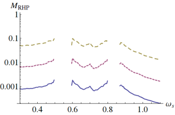
Figure 6: RHP non-Markovianity against system frequency $\omega_{s}$ comparing the result with $r=1,2,3$ (continuous, dashed, dashed-dashed). The behavior is the same, only with higher absolute values.

The main issue with this measure is that for low system-bath couplings it is inconclusive (i.e. $M_{RHP}=0$), but this can be easily fixed by increasing $k$. Typical time steps for integration of this measure $\delta t=0.1$ (e.g. for $\tau_{R}\sim 700$ in Fig.3) have been used, which is more than enough to resolve the positive slopes of the dynamics for $E_{SA}$ (see eq. (4) in main work).

Figure 7: BLP non-Markovianity as used for the figures related to temperature, for $T=0,0.5,1$ and $\omega_{s}=0.375$. It can be seen that for higher temperatures several maxima appear at different squeezing parameters $r_{2},\theta_{2}$.

The simulations for $M_{BLP}$ have been performed between pairs of one-mode vacuum squeezed states. In Fig.3 of main work, one of them having squeezing parameter $r_{1}=1$ and phase-space angle $\theta_{1}=0$, the other state having $r_{2}\in[0.5,1]$, $\Delta r_{2}=0.5$ and $\theta_{2}\in[0,\pi/2]$ with $\Delta\theta_{2}=\pi/4$ (same for Fig. 4c; for Figs. 4d and 5 we have used $r_{2}\in[0.25,1]$ with $\Delta r_{2}=0.25$). The bold (blue) point in Fig. 3 in the main paper was obtained by increasing $r_{2}\in[0.125,1.125]$, $\Delta r_{2}=0.5$ and $\theta_{2}\in[0,\pi/2]$ with $\Delta\theta_{2}=\pi/4$. Instead, for figures 4a,b we have used a much more thorough scan with $r_{1}=1/3,1$, $\theta_{1}=0$, $r_{2}\in[0,2]$, $\Delta r_{2}=0.1$ and $\theta_{2}\in[0,\pi]$ with $\Delta\theta_{2}=\pi/10$. We stress that the behavior against temperature is quite sensitive to the range of squeezings used and needs to be scanned intensively, because the optimal pair for this measure depends on the bath temperature (mostly for low T). We show an example in Fig. 7.

NM behavior with non-Ohmic bath for other parametrizations

The behavior of $M_{BLP}$ under the non-Ohmic spectral density

$$J(\omega)=k(\omega/\omega_{s})^{s}\Theta(\omega-0.25)\Theta(0.75-\omega)$$ (13)

was shown in last figure of main work, Fig. 5. This is a spectral density which pivots around $\omega_{s}$ and therefore keeps the coupling strength ($J(\omega_{S})=k\ ,\forall s$) fixed, while at the same time the extreme points ($\omega_{0}$ and $\omega_{R}$) it differs in values. However, choosing for example

$$J(\omega)=k(\omega-\omega_{0})^{s}\Theta(\omega_{R}-\omega)$$ (14)

(which keeps $J(\omega_{0})$ constant but differs at $J(\omega_{R})$ for different $s$) would change the value of $M_{BLP}$, as shown in Fig. 8.

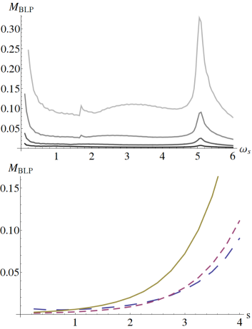
Figure 8: Top: BLP non-Markovianity against system frequency $\omega_{s}$ with $J(\omega)=k(\omega-\omega_{0})^{s}\Theta(\omega_{R}-\omega)$, $\omega_{0}=1$, $\omega_{R}=5$ and $s=1,2,3,4$ (black for $s=1$ to gray for $s=4$. Bottom: BLP NM versus $s$ evaluated at $\omega_{s}=1,3,5$ (sparse dashed, tight dashed, continuous) for the spectral density above.

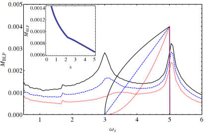
Figure 9: BLP non-Markovianity against system frequency $\omega_{s}$ with $J(\omega)=k[(\omega-\omega_{0})/(\omega_{R}-\omega_{0})]^{s}\Theta(\omega_{R}-\omega)$, $\omega_{0}=3$, $\omega_{R}=5$ and $s=1/2,1,2$ (continuous, dashed, dotted). We have drawn the spectral density to guide the eye. Inset: BLP NM versus $s$ evaluated at $\omega_{s}=4$.

Deeper differences are found considering different power law spectra densities with constraint coupling strengths at both $\omega_{0}$ and $\omega_{R}$, as results from

$$J(\omega)=k[(\omega-\omega_{0})/(\omega_{R}-\omega_{0})]^{s}\Theta(\omega_{R}-\omega).$$ (15)

In Fig. 9 it can be seen that the behavior of $M_{BLP}$ is again different. It does actually decrease in the super-ohmic case (larger $s$ values).

We notice that in the latter two cases the spectral density at the system frequency $J(\omega_{S})$ differs in value when changing $s$, unlike the case discussed in the main work. These examples show that normalization has to be carefully taken into account when drawing general conclusions about non-Markovian aspects of dissipation in presence of different power law in the spectral density.