A Time-Dependent Dirichlet-Neumann Method for the Heat Equation

1 Introduction

We introduce a new Waveform Relaxation (WR) method based on the Dirichlet-Neumann algorithm and present convergence results for it in one space dimension. To solve time-dependent problems in parallel, one can either discretize in time to obtain a sequence of steady problems to which the domain decomposition algorithms are applied, or apply WR to the large system of ordinary differential equations (ODEs) obtained from spatial discretization. The credit of WR method goes to Picard mandalb_mini15_Picard and Lindelöf mandalb_mini15_Lind for the solution of ODEs in the late 19th century. Lelarasmee, Ruehli and Sangiovanni-Vincentelli mandalb_mini15_LelRue were the first to introduce the WR as a parallel method for the solution of ODEs. The main advantage of the WR method is that one can use different time steps in different space-time subdomains. The authors of mandalb_mini15_GanStu and mandalb_mini15_GilKel then generalized WR methods for ODEs to solve time-dependent PDEs. Gander and Stuart mandalb_mini15_GanStu showed linear convergence of overlapping Schwarz WR iteration for the heat equation on unbounded time intervals with a rate depending on the size of the overlap; Giladi and Keller mandalb_mini15_GilKel proved superlinear convergence of the Schwarz WR method with overlap for the convection-diffusion equation on bounded time intervals.

The Dirichlet-Neumann method, which belongs to the class of substructuring methods, is based on a non-overlapping spatial domain decomposition. The iteration involves subdomain solves with Dirichlet boundary conditions, followed by subdomain solves with Neumann boundary conditions. The Dirichlet-Neumann algorithm was first considered for elliptic problems by P. E. Bjørstad & O. Widlund mandalb_mini15_BjPetter and further discussed in mandalb_mini15_BramPas , mandalb_mini15_MarQuar02 and mandalb_mini15_MarQuar01 . In this paper, we propose the Dirichlet-Neumann Waveform Relaxation (DNWR) method, a new Dirichlet-Neumann analogue of WR for the time-dependent problems. For presentation purposes, we derive our results for two subdomains in one spatial dimension. We discuss the method in the continuous setting to ensure the understanding of the asymptotic behavior of the method in the case of fine grids.

We consider the following initial boundary value problem (IBVP) for the heat equation as our guiding example on a bounded domain $\Omega\subset\mathbb{R},0<t<T$,

$$\begin{array}[]{rcll}\frac{\partial u}{\partial t}&=&\Delta u+f(x,t),&x\in\Omega,0<t<T,\\ u(x,0)&=&u_{0}(x),&x\in\Omega,\\ u(x,t)&=&g(x,t),&x\in\partial\Omega,0<t<T.\end{array}$$ (1)

2 The Dirichlet-Neumann Waveform Relaxation algorithm

To define the Dirichlet-Neumann iterative method for the model problem (1) on the domain $(-b,a)\times(0,T)$, we split the spatial domain $\Omega=(-b,a)$ into two non-overlapping subdomains, the Dirichlet subdomain $\Omega_{1}=(-b,0)$ and the Neumann subdomain $\Omega_{2}=(0,a)$, for $0<a,b<\infty$. The Dirichlet-Neumann Waveform Relaxation algorithm consists of the following steps: given an initial guess $h^{0}(t),t\in(0,T)$ along the interface $\Gamma=\left\{x=0\right\}$ and for $k=0,1,2,\ldots$, do

$$\begin{cases}\partial_{t}u_{1}^{k+1}-\partial_{xx}u_{1}^{k+1}=f(x,t),&x\in\Omega_{1},\\ u_{1}^{k+1}(x,0)=u_{0}(x),&x\in\Omega_{1},\\ u_{1}^{k+1}(-b,t)=g(-b,t),\\ u_{1}^{k+1}(0,t)=h^{k}(t),\end{cases}\begin{cases}\partial_{t}u_{2}^{k+1}-\partial_{xx}u_{2}^{k+1}=f(x,t),&x\in\Omega_{2},\\ u_{2}^{k+1}(x,0)=u_{0}(x),&x\in\Omega_{2},\\ \partial_{x}u_{2}^{k+1}(0,t)=\partial_{x}u_{1}^{k+1}(0,t),\\ u_{2}^{k+1}(a,t)=g(a,t),\end{cases}$$ (2)

with the updating condition

$$h^{k+1}(t)=\theta u_{2}^{k+1}(0,t)+(1-\theta)h^{k}(t),$$ (3)

$\theta$ being a positive relaxation parameter. The parameter $\theta$ is chosen in $(0,1]$ to accelerate convergence. As the main goal of the analysis is to study how the error $h^{k}(t)-u(0,t)$ converges to zero, by linearity it suffices to consider the homogeneous problem, $f(x,t)=0$, $g(x,t)=0$, $u_{0}(x)=0$ in (1), and examine how $h^{k}(t)$ goes to zero as $k\rightarrow\infty$.

3 Convergence analysis and main results

We analyze the DNWR algorithm using the Laplace transform method. The Laplace transform of a function $w(t)$, defined for all real numbers $t\in[0,\infty)$, is the function $\hat{w}(s)$, defined by

$$\hat{w}(s)=\mathcal{L}\left\{w(t)\right\}:=\int_{0}^{\infty}e^{-st}w(t)\,dt,$$

(if the integral exists) $s$ being a complex variable. If $\mathcal{L}\left\{w(t)\right\}=\hat{w}(s)$, then the inverse Laplace transform of $\hat{w}(s)$ is denoted by

$$\mathcal{L}^{-1}\left\{\hat{w}(s)\right\}:=w(t),\qquad t\geq 0,$$

which maps the Laplace transform of a function back to the original function. For more information on Laplace transforms, see mandalb_mini15_Church ; mandalb_mini15_Oberhett . We use hats to denote the Laplace transform of a function in time in the rest of the paper.
Analysis by Laplace transforms. Applying a Laplace transform in time to (2) and solving the resulting ODEs yields the solutions: $\hat{u}_{1}^{k+1}(x,s)=\frac{\hat{h}^{k}(s)}{\sinh(b\sqrt{s})}\sinh\left\{(x+b)\sqrt{s}\right\}$ and $\hat{u}_{2}^{k+1}(x,s)=\hat{h}^{k}(s)\frac{\coth(b\sqrt{s})}{\cosh(a\sqrt{s})}\sinh\{(x-a)\sqrt{s}\}.$ Now, evaluating $\hat{u}_{2}^{k+1}(x,s)$ at $x=0$ and inserting it into the transformed updating condition (3), we get for $k=0,1,2,\ldots$ $\hat{h}^{k+1}(s)=\left\{1-\theta-\theta\tanh(a\sqrt{s})\coth(b\sqrt{s})\right\}\hat{h}^{k}(s).$ Therefore, by induction we get

$$\hat{h}^{k}(s)=\left\{1-\theta-\theta\tanh(a\sqrt{s})\coth(b\sqrt{s})\right\}^{k}\hat{h}^{0}(s),\quad k=1,2,3,...$$ (4)

Theorem 3.1

For the symmetric case, $a=b$ in (2)-(3), the DNWR algorithm converges linearly for $0<\theta<1$. Moreover, for $\theta=0.5$, it converges to the exact solution in two iterations, independent of the size of the time window.

Proof

For $a=b$, the equation (4) reduces to $\hat{h}^{k}(s)=(1-2\theta)^{k}\hat{h}^{0}(s),$ which upon back transforming gives $h^{k}(t)=(1-2\theta)^{k}h^{0}(t)$. Thus, the convergence is linear for $\theta\neq 0.5$. On the other hand, for $\theta=0.5$, $h^{1}(t)=0$. Therefore, one more iteration produces the desired solution on the whole domain.$\hfill\qed$

The main area of concern for the rest of the paper is the analysis of the DNWR algorithm for $a\neq b$. If we define

$$G(s):=\tanh(a\sqrt{s})\coth(b\sqrt{s})-1=\frac{\sinh((a-b)\sqrt{s})}{\cosh(a\sqrt{s})\sinh(b\sqrt{s})},$$

then the recurrence relation (4) reduces to

$$\hat{h}^{k}(s)=\begin{cases}\left\{q(\theta)-\theta G(s)\right\}^{k}\hat{h}^{0}(s),&\theta\neq 1/2\\ (-1)^{k}2^{-k}G^{k}(s)\hat{h}^{0}(s),&\theta=1/2,\end{cases}$$ (5)

where $q(\theta)=1-2\theta.$ Note that for $\textrm{Re}(s)>0,$ $G(s)$ is $\mathcal{O}(s^{-p})$ for every positive $p$. Therefore, by (mandalb_mini15_Church, , p. 178), $G(s)$ is the Laplace transform of an analytic function $F_{1}(t)$ (in fact this is the motivation in defining $G$). In general, define $F_{k}(t):=\mathcal{L}^{-1}\left\{G^{k}(s)\right\}$ for $k=1,2,3,\ldots$. For $\theta$ not equal to $1/2$, $h^{k}$ cannot be expressed as a simple convolution of $h^{0}$ and an analytic function; thus, different techniques are required to analyze its behavior. This case will be treated in a future paper. For $\theta=1/2$ and $t\in(0,T)$ we get from (5)

$$\bigl{|}h^{k}(t)\bigr{|}=\biggl{|}2^{-k}\int_{0}^{t}(-1)^{k}h^{0}(t-\tau)F_{k}(\tau)d\tau\biggr{|}\leq 2^{-k}\parallel h^{0}\parallel_{L^{\infty}(0,T)}\int_{0}^{T}\Bigl{|}F_{k}(\tau)\Bigr{|}d\tau.$$ (6)

So, we need to bound $\int_{0}^{T}\bigl{|}F_{k}(\tau)\bigr{|}d\tau$ to get an $L^{\infty}$ convergence estimate. We concentrate on showing that $F_{1}(t)$ does not change signs both for the case $b<a$, in which $F_{1}(t)\geq 0$, and for $b\geq a$, for which $F_{1}(t)\leq 0$. Before we proceed further with the proof we need the following lemmas.

Lemma 1

Let, $w(t)$ be a continuous and $L^{1}$-integrable function on $(0,\infty)$ with $w(t)\geq 0$ for all $t\geq 0$. Assume $W(s)=\mathcal{L}\left\{w(t)\right\}$. Then, for $\tau>0,$

$$\int_{0}^{\tau}|w(t)|dt\leq{\displaystyle\lim_{s\rightarrow 0+}}W(s).$$

Proof

Using the definition of Laplace transform, we have

$$\int_{0}^{\tau}|w(t)|dt=\int_{0}^{\tau}w(t)dt \leq\int_{0}^{\infty}w(t)dt$$

$$=\int_{0}^{\infty}{\displaystyle\lim_{s\rightarrow 0+}}e^{-st}w(t)dt ={\displaystyle\lim_{s\rightarrow 0+}}\int_{0}^{\infty}e^{-st}w(t)dt\;\mbox{(by Dominated Conv. Theorem)}$$

$$={\displaystyle\lim_{s\rightarrow 0+}}W(s).\quad\quad\quad\quad\quad\quad\quad\qed$$

Lemma 2

Let $\beta>\alpha\geq 0$ and $s$ be a complex variable. Then, for $t\in(0,\infty)$

$$\varphi(t):=\mathcal{L}^{-1}\left\{\frac{\sinh(\alpha\sqrt{s})}{\sinh(\beta\sqrt{s})}\right\}\geq 0\;;\;\>\psi(t):=\mathcal{L}^{-1}\left\{\frac{\cosh(\alpha\sqrt{s})}{\cosh(\beta\sqrt{s})}\right\}\geq 0.$$

Proof

First, let us consider the following IBVP for the heat equation on $(0,\beta)$: $u_{t}-u_{xx}=0,\,u(x,0)=0,\>u(0,t)=0,\>u(\beta,t)=g(t).$ Therefore, for $g$ non-negative, $u(\alpha,t)$ is also non-negative for all $t>0$, thanks to the maximum principle. Now using the Laplace transform method, we get the solution along $x=\alpha$ as

$$\hat{u}(\alpha,s)=\hat{g}(s)\frac{\sinh(\alpha\sqrt{s})}{\sinh(\beta\sqrt{s})}\quad\Longrightarrow\quad u(\alpha,t)=\int_{0}^{t}g(t-\tau)\varphi(\tau)d\tau.$$

We prove the result by contradiction: suppose $\varphi(t_{0})<0$ for some $t_{0}>0$. Then by continuity of $\varphi$, there exists $\delta>0$ such that $\varphi(\tau)<0,$ for $\tau\in(t_{0}-\delta,t_{0}+\delta)$. Now for $t>t_{0}+\delta$, we choose $g$ as

$$g(\varsigma)=\begin{cases}1,&\varsigma\in\left(t-t_{0}-\delta,t-t_{0}+\delta\right)\\ 0,&\textrm{else}.\end{cases}$$

Then $u(\alpha,t)=\int_{t_{0}-\delta}^{t_{0}+\delta}g(t-\tau)\varphi(\tau)d\tau=\int_{t_{0}-\delta}^{t_{0}+\delta}\varphi(\tau)d\tau<0$, a contradiction. This proves $\varphi$ to be non-negative. For $\psi$, applying the Laplace transform method to the IBVP for the heat equation $u_{t}-u_{xx}=0,\>u(x,0)=0,\>u(-\beta,t)=g(t),\>u(\beta,t)=g(t)$ yields the solution along $x=\alpha$ as: $\hat{u}(\alpha,s)=\hat{g}(s)\frac{\cosh(\alpha\sqrt{s})}{\cosh(\beta\sqrt{s})}$. Thus, a similar argument as in the first case proves that $\psi$ is also non-negative.$\hfill\qed$

Theorem 3.2

(Linear convergence bound for the Heat equation) Let $\theta=1/2$. For $T>0$, the error of the Dirichlet-Neumann Waveform Relaxation (DNWR) algorithm satisfies

$$\parallel h^{k}\parallel_{L^{\infty}(0,T)}\leq\left(\frac{|b-a|}{2b}\right)^{k}\parallel h^{0}\parallel_{L^{\infty}(0,T)}.$$

We therefore have a contraction if $a<3b.$

Proof

By virtue of (6), it is sufficient to bound $\int_{0}^{T}\bigl{|}F_{k}(\tau)\bigr{|}d\tau$ for both $b\geq a$ and $a>b$, where $F_{k}(t)=\mathcal{L}^{-1}\left\{G^{k}(s)\right\}$. Suppose $b\geq a>0.$ We have $\mathcal{L}\left\{-F_{1}(t)\right\}=\frac{\sinh((b-a)\sqrt{s})}{\sinh(b\sqrt{s})}\cdot\frac{1}{\cosh(a\sqrt{s})}.$ So by Lemma 2 and the fact that the convolution of two positive functions is positive, $-F_{1}(t)$ is positive. Thus, by induction and with the same arguments, $(-1)^{k}F_{k}(t)\geq 0$ for all $t$. Therefore by Lemma 1

$$\int_{0}^{T}\bigl{|}(-1)^{k}F_{k}(\tau)\bigr{|}d\tau\leq{\displaystyle\lim_{s\rightarrow 0+}}(-1)^{k}G^{k}(s)=\left(\frac{b-a}{b}\right)^{k}.$$ (7)

Now let $a>b>0$. We claim that $F_{1}(t)$ is positive. If $a-b\leq b$, then we get the positivity by Lemma 2. If this is not the case, then take the integer $m=\lfloor a/b\rfloor$ so that $mb<a\leq(m+1)b$. Then, recursively applying the identity

$$\frac{\sinh((a-jb)\sqrt{s})}{\sinh(b\sqrt{s})}=\frac{\sinh((a-(j+1)b)\sqrt{s})}{\sinh(b\sqrt{s})}\cosh(b\sqrt{s})+\cosh((a-(j+1)b)\sqrt{s})$$

for $j=1,\ldots,m-1$, we obtain

$$\frac{\sinh((a-b)\sqrt{s})}{\cosh(a\sqrt{s})\sinh(b\sqrt{s})}=\frac{\sinh((a-mb)\sqrt{s})}{\sinh(b\sqrt{s})}.\frac{\cosh^{m-1}(b\sqrt{s})}{\cosh(a\sqrt{s})}\\ +{\displaystyle\sum_{j=0}^{m-2}}\frac{\cosh^{j}(b\sqrt{s})\cosh\left((a-(j+2)b)\sqrt{s}\right)}{\cosh(a\sqrt{s})}.$$

Applying the binomial theorem to $\cosh\theta=\left(e^{\theta}+e^{-\theta}\right)/2$ we have the power-reduction formula

$$\cosh^{n}\theta=\begin{cases}\frac{2}{2^{n}}{\displaystyle\sum_{l=0}^{\frac{n-1}{2}}}\binom{n}{l}\cosh\left((n-2l)\theta\right),&n\>\>\textrm{odd},\\ \frac{1}{2^{n}}\binom{n}{n/2}+\frac{2}{2^{n}}{\displaystyle\sum_{l=0}^{\frac{n}{2}-1}}\binom{n}{l}\cosh\left((n-2l)\theta\right),&n\>\>\textrm{even},\end{cases}$$

so that we can write $\cosh^{n}\theta={\displaystyle\sum_{l=0}^{n}}A_{l}^{n}\cosh\left(l\theta\right)$ with ${\displaystyle\sum_{l=0}^{n}}A_{l}^{n}=1$ and $A_{l}^{n}\geq 0$. Therefore, we have

$$G(s)=\frac{\sinh((a-b)\sqrt{s})}{\cosh(a\sqrt{s})\sinh(b\sqrt{s})}=\frac{\sinh((a-mb)\sqrt{s})}{\sinh(b\sqrt{s})}{\displaystyle\sum_{l=0}^{m-1}}A_{l}^{m-1}\frac{\cosh(lb\sqrt{s})}{\cosh(a\sqrt{s})}\\ +{\displaystyle\sum_{j=0}^{m-2}}{\displaystyle\sum_{l=0}^{j}}\frac{A_{l}^{j}}{2}\left\{\frac{\cosh\left((a-(j+l+2)b)\sqrt{s}\right)}{\cosh(a\sqrt{s})}+\frac{\cosh\left((a-(j-l+2)b)\sqrt{s}\right)}{\cosh(a\sqrt{s})}\right\},$$

where $\cosh^{j}\theta={\displaystyle\sum_{l=0}^{j}}A_{l}^{j}\cosh\left(l\theta\right)$. Note that $a-mb\leq b$, $(j-l+2)b\leq mb<a$ and $\left|a-(j+l+2)b\right|<a$ for $0\leq j,l\leq m-2$ and $\cosh$ is an even function. Thus by Lemma 2, each term in the above expression is the Laplace transform of a positive function. Hence $F_{1}(t)$ is positive, and therefore the convolution of $k$ $F_{1}$’s (i.e. $F_{k}(t)$) is also positive. We have ${\displaystyle\lim_{s\rightarrow 0+}}G(s)={\displaystyle\lim_{s\rightarrow 0+}}\frac{\sinh((a-b)\sqrt{s})}{\cosh(a\sqrt{s})\sinh(b\sqrt{s})}=\frac{a-b}{b},$ and so by Lemma 1

$$\int_{0}^{T}\bigl{|}F_{k}(\tau)\bigr{|}d\tau=\int_{0}^{T}F_{k}(\tau)d\tau\leq{\displaystyle\lim_{s\rightarrow 0+}}G^{k}(s)=\left({\displaystyle\lim_{s\rightarrow 0+}}G(s)\right)^{k}=\left(\frac{a-b}{b}\right)^{k}.$$ (8)

The result follows by inserting the estimates (7) and (8) into (6). $\hfill\qed$

4 Numerical Experiments

We perform experiments to measure the actual convergence rate of the DNWR algorithm for the problem

$$\begin{cases}\frac{\partial u}{\partial t}-\frac{\partial^{2}u}{\partial x^{2}}=-e^{-t-x^{2}},&x\in(-3,2),\\ u(x,0)=e^{-2x},&x\in(-3,2),\\ u(-3,t)=e^{-2t}=u(2,t),&t>0.\end{cases}$$

To solve the equation using the Dirichlet-Neumann algorithm, we discretize the Laplacian using centered finite differences in space and backward Euler in time on a grid with $\Delta x=2\times 10^{-2}$ and $\Delta t=4\times 10^{-4}$. For the numerical experiments we split the spatial domain into two non-overlapping subdomains $\left[-3,0\right]$ and $\left[0,2\right]$, so that $b=3$ and $a=2$ in (2)-(3). Thus this is the case when the Dirichlet subdomain is bigger than the Neumann subdomain. The numerical results are similar for the case when the Neumann domain is larger than the Dirichlet one. We test the algorithm by choosing $h^{0}(t)=t$, $t\in(0,T]$ as an initial guess. Figure 1 gives the error reduction curves for different values of the parameter $\theta$ for $T=2$ in $(a)$ and $T=200$ in $(b)$. Note that, for a small time window, we get linear convergence for all the parameters, except for $\theta=0.5$ which corresponds to superlinear convergence.

 

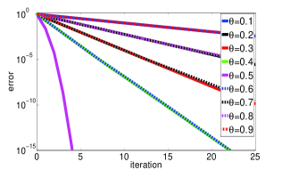
(a) Short time window

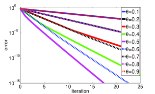
(b) Large time window

Figure 1: Convergence for various parameters; left: short time window, right: large time window.

For a large time window, we always observe linear convergence. We now plot the linear bound for the convergence rate in case of $\theta=1/2$ as shown in Theorem 2. The theorem provides a $T$-independent theoretical bound of the error for this special relaxation parameter and this is also valid for large time windows. Eventually, a more refined analysis will give a superlinear bound shown in (9)-(10), dependent on $T$ and the lengths of the subdomains (see mandalb_mini15_GKM ). Figure 2 gives a comparison between the theoretical error for the continuous model problem (calculated using inverse Laplace transforms), numerical error for the discretized problem, linear bound and the superlinear bound for $a=2,b=3$ and various $T$’s. We can observe that the error curves seem to approach the linear bound as $T$ increases.

 

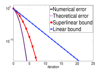
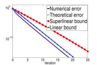
Figure 2: Bounds for various times, $b\geq a$; in particular $a<3b$. Left: $T=2$, right: $T=200$

5 Conclusions and further results

We proved convergence of the proposed DNWR algorithm in the symmetric case. For unequal subdomain lengths and for a particular choice of relaxation parameter, we presented a linear error estimate that is valid for both bounded and unbounded time intervals. In fact, Figure 2 suggests that the method converges superlinearly.

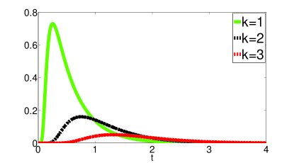
Figure 3: $F_{k}(t),k=1,2,3.$

To prove this, one has to consider two different cases: Dirchlet subdomain bigger than Neumann subdomain ($b\geq a$) and the other way around. Figure 3 shows $F_{k}(t)$ for $k=1,2,3$; we see that the curves shift to the right and at the same time, the peak decreases as $k$ increases. So, if one only considers a small time window, the peak will eventually exit the time window for $k$ large enough and its contribution will be vanishingly small in the expression (5). This is the intuitive idea to get superlinear convergence for $\theta=1/2$ in small time windows. A detailed analysis, which is too long for this short paper, in mandalb_mini15_GKM leads to the following superlinear convergence estimates for the small time window $(0,T)$:

$$\parallel h^{k}\parallel_{L^{\infty}(0,T)}\leq\left(\frac{b-a}{b}\right)^{k}\textrm{erfc}\left(\frac{ka}{2\sqrt{T}}\right)\parallel h^{0}\parallel_{L^{\infty}(0,T)},\quad\mbox{for}\;b\geq a,$$ (9)

and

$$\parallel h^{2k}\parallel_{L^{\infty}(0,T)}\leq\left\{\frac{\sqrt{2}}{1-e^{-\frac{2k+1}{\sigma}}}\right\}^{2k}e^{-k^{2}/\sigma}\parallel h^{0}\parallel_{L^{\infty}(0,T)},\quad\mbox{for}\;b<a,$$ (10)

where $\sigma=T/b^{2}.$ We are also working on a generalization of the algorithm to higher dimensions.

- (1) Bjørstad, P.E., Widlund, O.B.: Iterative Methods for the Solution of Elliptic Problems on Regions Partitioned into Substructures. SIAM J. Numer. Anal. (1986)
- (2) Bramble, J.H., Pasciak, J.E., Schatz, A.H.: An Iterative Method for Elliptic Problems on Regions Partitioned into Substructures. Mathematics of Computation (1986)
- (3) Churchill, R.V.: Operational Mathematics, 2nd edn. McGraw-Hill (1958)
- (4) Gander, M.J.: Optimized Schwarz methods. SIAM J. Numer. Anal. 44(2), 699–732 (2006)
- (5) Gander, M.J., Kwok, F., Mandal, B.C.: Dirichlet-Neumann and Neumann-Neumann Waveform Relaxation Methods for the Heat Equation. (In Preparation)
- (6) Gander, M.J., Stuart, A.M.: Space-time continuous analysis of waveform relaxation for the heat equation. SIAM J. for Sci. Comput. 19(6), 2014–2031 (1998)
- (7) Giladi, E., Keller, H.: Space time domain decomposition for parabolic problems. Numer. Math. 93, 279–313 (2002)
- (8) Lelarasmee, E., Ruehli, A., Sangiovanni-Vincentelli, A.: The waveform relaxation method for time-domain analysis of large scale integrated circuits. IEEE Trans. Compt.-Aided Design Integr. Circuits Syst. 1(3), 131–145 (1982)
- (9) Lindelöf, E.: Sur l’application des méthodes d’approximations successives à l’étude des intégrales réelles des équations différentielles ordinaires. Journal de Mathématiques Pures et Appliquées (1894)
- (10) Lions, P.L.: On the Schwarz alternating method. in First International Symposium on Domain Decomposition Methods for PDEs, I (3) (1989)
- (11) Martini, L., Quarteroni, A.: An iterative procedure for domain decomposition methods: a finite element approach. SIAM, in Domain Decomposition Methods for PDEs, I pp. 129–143 (1988)
- (12) Martini, L., Quarteroni, A.: A Relaxation Procedure for Domain Decomposition Method using Finite Elements. Numer. Math. (1989)
- (13) Oberhettinger, F., Badii, L.: Tables of Laplace Transforms. Springer-Verlag (1973)
- (14) Picard, E.: Sur l’application des méthodes d’approximations successives à l’étude de certaines équations différentielles ordinaires. Journal de Mathématiques Pures et Appliquées (1893)