On the Practical Application of Physical Anomalous Dimensions

Abstract

We revive the idea of using physical anomalous dimensions in the QCD scale evolution of deep-inelastic structure functions and their scaling violations and present a detailed phenomenological study of its applicability. Differences with results obtained in the conventional framework of scale-dependent quark and gluon densities are discussed and traced back to the truncation of the perturbative series at a given order in the strong coupling.

I Introduction and Motivation

Measurements of deep-inelastic scattering (DIS) cross sections are routinely analyzed in terms of scale-dependent quark and gluon distribution functions $f_{i}(x,Q^{2})$, $i=q,\bar{q},g$ in global QCD fits ref:pdffits . In particular, the very accurate DIS data from the DESY-HERA experiments Aaron:2009aa provide the backbone of such type of QCD analyses, also thanks to their vast coverage in the relevant kinematic variables $x$ and $Q^{2}$, denoting the momentum fraction carried by the struck parton and the resolution scale set by the momentum transfer squared, respectively.

The conventional theoretical framework for DIS is based on the factorization theorem Collins:1989gx , which allows one to organize the computation of DIS structure functions $F_{2,L}(x,Q^{2})$ as a convolution of perturbatively calculable Wilson coefficients Furmanski:1981cw ; vanNeerven:1991nn ; Moch:1999eb ; Kazakov:1987jk and parton distribution functions (PDFs) capturing the long-distance, non-perturbative physics Blumlein:2012bf . Similar ideas are successfully applied to more complicated hard-scattering processes studied at hadron-hadron colliders, which provide further, invaluable constraints on PDFs in global QCD analyses ref:pdffits .

To make the separation between long- and short-distance physics manifest, one needs to introduce some arbitrary factorization scale $\mu_{f}$, apart from the scale $\mu_{r}$ appearing in the renormalization of the strong coupling $\alpha_{s}$. The independence of physical observables such as $F_{2,L}$ on $\mu_{f}$ can be used to derive powerful renormalization group equations (RGEs) governing the scale dependence of PDFs in each order of perturbation theory. The corresponding kernels are the anomalous dimensions or splitting functions associated with collinear two-parton configurations ref:lo ; ref:nlo ; ref:nnlo . Since factorization can be carried out in infinitely many different ways, one is left with an additional choice of the factorization scheme for which one usually adopts the $\overline{\mathrm{MS}}$ prescription Bardeen:1978yd . Likewise, the RGE governing the running of $\alpha_{s}$ with $\mu_{r}$ can be deduced from taking the derivative of $F_{2,L}$ with respect to $\mu_{r}$. Upon properly combining PDFs and Wilson coefficients in the same factorization scheme, any residual dependence on $\mu_{f}$ is suppressed by an additional power of $\alpha_{s}$, i.e., is formally one order higher in the perturbative expansion but not necessarily numerically small.

Alternatively, it is possible to formulate QCD scale evolution equations directly for physical observables without resorting to auxiliary, convention-dependent quantities such as PDFs. This circumvents the introduction of a factorization scheme and $\mu_{f}$ and, hence, any dependence of the results on their actual choice. The concept of physical anomalous dimensions is not at all a new idea and has been proposed quite some time ago Furmanski:1981cw ; Catani:1996sc ; Blumlein:2000wh but its practical aspects have never been studied in detail. The framework is suited best for theoretical analyses based on DIS data with the scale $\mu_{r}$ in the strong coupling being the only theoretical ambiguity. In addition, $F_{2,L}$ or their scaling violations can be parametrized much more economically than a full set of quark and gluon PDFs, which greatly simplifies any fitting procedure and phenomenological analysis. The determination of $\alpha_{s}$ from fits to DIS structure functions is the most obvious application, as theoretical scheme and scale uncertainties are reduced to a minimum. We note that physical anomalous dimension were used, however, also as a calculational tool to study, e.g., all-order aspects of the perturbative series for splitting and coefficient functions in the limit of large momentum fractions $x$ Soar:2009yh .

Recently, the interest in DIS has been revived in a series of dedicated studies in search of a compelling physics case for a future high-luminosity electron-ion collider, such as the proposed EIC Boer:2011fh and LHeC AbelleiraFernandez:2012ni projects. One of the driving physics goals is a detailed mapping of the transition into a non-linear kinematic regime dominated by high, or saturated, gluon densities by measuring, for instance, $F_{2,L}$ and their scaling violations very precisely at small $x$ both in electron-proton and in electron-heavy ion collisions. A signature for the onset of saturation effects would be the observation of deviations from the linear, Dokshitzer-Gribov-Lipatov-Altarelli-Parisi (DGLAP) type of QCD scale evolution, which, again, could be identified best by performing analyses in the framework of physical anomalous dimensions.

In this paper we will largely focus on the practical implementation of physical anomalous dimensions in analyses of DIS data up to next-to-leading order (NLO) accuracy. We shall study in detail potential differences with results obtained in the conventional framework based on scale-dependent quark and gluon densities, which could be caused by the way how the perturbative series is truncated at any given order. To the best of our knowledge, these practical aspects have never been studied before, apart from a brief application of physical anomalous dimensions in an attempt to extract the strong coupling from DIS structure function data taken with longitudinally polarized leptons and hadrons Bluemlein:2002be .

The results obtained in this note should provide the framework for using physical anomalous dimensions in actual quantitative phenomenological studies to be pursued once data from a future electron-ion collider become available or for projections based on pseudo-data. Apart from the applications related to gluon saturation, precise data for the longitudinally polarized DIS structure function $g_{1}$ and its scaling violations $dg_{1}/d\ln Q^{2}$ are expected from an EIC Boer:2011fh ; Aschenauer:2012ve . Such data should allow one to revisit the attempted extraction of $\alpha_{s}$ performed in Ref. Bluemlein:2002be . We note that physical anomalous dimensions can be also applied to time-like processes such as inclusive hadron production in electron-positron annihilation. These processes are traditionally parametrized by fragmentation functions, which account for the non-perturbative transition of a certain quark flavor or gluon into the observed hadron species deFlorian:2007aj . Again it is in principle possible to use time-like equivalents of DIS structure functions and evolve them in a factorization scheme independent way.

The paper is organized as follows: in Section II we briefly recall how to derive physical anomalous dimensions to establish our notation and conventions used throughout the paper. Explicit results are given in leading and next-to-leading order of perturbation theory and compared with the results known in the literature. In Section III we discuss the numerical implementation, outline subtleties related to the truncation of the perturbative series at NLO, and show how to circumvent them. We briefly summarize our results in Section IV.

II Theoretical Framework

This gist of the factorization scheme-invariant framework amounts to combine any two DIS observables $\{F_{A},F_{B}\}$ and determine their corresponding $2\times 2$ matrix of physical anomalous dimensions in lieu of the scale-dependent quark singlet, $\Sigma\equiv\sum_{q}(q+\bar{q})$, and gluon distributions appearing in the standard, coupled singlet DGLAP evolution equations. Instead of using measurements of $F_{2}$ and $F_{L}$ (actually their flavor singlet parts), one can also utilize their variation with scale for any given value of $x$, i.e., $dF_{2,L}(x,Q^{2})/d\ln Q^{2}$ as an observable. The required sets of physical anomalous dimensions for both $\{F_{2},F_{L}\}$ and $\{F_{2},dF_{2}/d\ln Q^{2}\}$ have been derived in Blumlein:2000wh up to NLO accuracy. The additionally needed evolution equations for the non-singlet portions of the structure functions $F_{2,L}$ are simpler and not matrix valued.

II.1 Physical Anomalous Dimensions

As we shall see below, the required physical anomalous dimensions comprise the inverse of coefficient and splitting functions and are most conveniently expressed in Mellin $n$ moment space. The Mellin transformation of a function $\phi$ given in Bjorken $x$ space, such as PDFs or splitting functions, is defined as

$$\phi(n)\equiv\int_{0}^{1}dx\,x^{n-1}\phi(x)\;,$$ (1)

where $n$ is complex valued. As an added benefit, convolutions in $x$ space turn into ordinary products upon applying (1), which, in turn, allows for an analytic solution of QCD scale evolution equations for PDFs. The corresponding inverse Mellin transformation is straightforwardly performed numerically along a suitable contour in $n$ space, see, e.g., Ref. Vogt:2004ns for details. The necessary analytic continuations to non-integer $n$ moments are given in Gluck:1989ze ; Blumlein:2000hw , and an extensive list of Mellin transforms is tabulated in Blumlein:1998if . We will work in Mellin space throughout this paper.

Assuming factorization, moments of DIS structure functions $F_{I}$ at a scale $Q$ can be expressed as

$$F_{I}(n,Q^{2})=\sum_{k=q,\bar{q},g} e_{k}^{2}\,C_{I,k}\left(n,a_{s}(\mu_{r}^{2}),\frac{Q^{2}}{\mu_{f}^{2}},\frac{\mu_{r}^{2}}{\mu_{f}^{2}}\right)\,$$

$$\cdot f_{k}\left(n,a_{s}(\mu_{r}^{2}),\frac{\mu_{f}^{2}}{Q_{0}^{2}},\frac{\mu_{r}^{2}}{\mu_{f}^{2}}\right)$$ (2)

where the sum runs over all contributing $n_{f}$ active quark flavors with electric charge $e_{q}$ and the gluon $g$, each represented by a PDF $f_{k}$. For $e_{g}^{2}$, the averaged quark charge factor $\bar{e}_{f}^{2}=(1/n_{f})\sum_{q}e_{q}^{2}$ has to be used instead. $\mu_{r}$ and $\mu_{f}$ specify renormalization and factorization scale, respectively. The scale $Q_{0}$ defines the starting scale for the PDF evolution, where a set of non-perturbative input distributions needs to be specified. For simplicity we identify in the following the renormalization scale with the factorization scale, i.e., $\mu_{r}=\mu_{f}\equiv\mu$. The coefficient functions $C_{I,k}$ are calculable in pQCD Furmanski:1981cw ; vanNeerven:1991nn ; Moch:1999eb ; Kazakov:1987jk and exhibit the following series in $a_{s}\equiv\alpha_{s}/4\pi$

$$C_{I,k}\left(n,a_{s}(\mu^{2}),\frac{Q^{2}}{\mu^{2}}\right)=\sum_{m=m_{0}}a^{m}_{s}(\mu^{2})\;C^{(m)}_{I,k}\left(n,\frac{Q^{2}}{\mu^{2}}\right)\;,$$ (3)

where $m_{0}$ depends on the first non-vanishing order in $a_{s}$ in the expansion for the observable under consideration, e.g., $m_{0}=0$ for $F_{2}$ and $m_{0}=1$ for $F_{L}$.

Each PDF $f_{k}(n,\mu^{2}/Q_{0}^{2})$ obeys the DGLAP evolution equation which reads

$$\frac{d}{d\ln\mu^{2}}f_{k}\left(n,\frac{\mu^{2}}{Q_{0}^{2}}\right)=\sum_{l=q,\bar{q},g}P_{kl}\left(n,a_{s}(\mu^{2})\right)f_{l}\left(n,\frac{\mu^{2}}{Q_{0}^{2}}\right)$$ (4)

where the $l\to k$ splitting functions have a similar expansion ref:lo ; ref:nlo ; ref:nnlo as the coefficient functions in Eq. (3):

$$P_{kl}(n,a_{s}(\mu^{2}))=\sum_{m=0}a_{s}(\mu^{2})^{1+m}\;P^{(m)}_{kl}(n)\;.$$ (5)

The $P_{kl}(n)$ relate to the corresponding anomalous dimensions through $\gamma_{kl}(n)=-2P_{kl}(n)$ in the normalization conventions we adopt, where we use the leading order (LO) and NLO expressions for $\gamma_{kl}(n)$ given in App. B of the first reference in ref:nlo . We note that the same normalization is used in the publicly available Pegasus evolution code Vogt:2004ns . In practice one distinguishes a $2\times 2$ matrix-valued DGLAP equation evolving the flavor singlet vector comprising $\Sigma(n,\mu^{2}/Q_{0}^{2})$ and $g(n,\mu^{2}/Q_{0}^{2})$ and a set of $n_{f}-1$ RGEs for the relevant non-singlet quark flavor combinations.

The scale-dependent strong coupling itself obeys another RGE governed by the QCD beta function

$$\frac{da_{s}(\mu)}{d\ln\mu^{2}}=\beta(a_{s})=-\sum_{m}a_{s}^{m+2}\beta_{m}$$ (6)

with $\beta_{0}=11-2n_{f}/3$ and $\beta_{1}=102-38n_{f}/3$ up to NLO accuracy. To compare below with the results for the physical anomalous dimensions in Ref. Blumlein:2000wh we also introduce the evolution variable

$$t\equiv-\frac{2}{\beta_{0}}\ln\left(\frac{a_{s}(Q^{2})}{a_{s}(Q_{0}^{2})}\right)\;.$$ (7)

Instead of studying $F_{I}(n,Q^{2})$ in (II.1) in terms of scale-dependent PDFs, which are obtained from solving the singlet and non-singlet combinations of DGLAP equations (4) in a fit to data ref:pdffits , one can also derive evolution equations directly in terms of the observables $F_{I}(n,Q^{2})$. To this end, we consider a pair of DIS observables $F_{A}$ and $F_{B}$, to be specified below, whose scale dependence is governed by a coupled matrix-valued equation

$$\frac{d}{d\ln Q^{2}}\begin{pmatrix}F_{A}^{(S)}(n,Q^{2})\\ F_{B}^{(S)}(n,Q^{2})\end{pmatrix}=$$

$$\begin{pmatrix}K_{AA}&K_{AB}\\ K_{BA}&K_{BB}\end{pmatrix}(n,a_{s}(Q^{2}))\cdot\begin{pmatrix}F_{A}^{(S)}(n,Q^{2})\\ F_{B}^{(S)}(n,Q^{2})\end{pmatrix}$$ (8)

for the flavor singlet (S) parts of $F_{A,B}$ and a set of non-singlet (NS) equations

$$\frac{dF_{A,B}^{(NS)}(n,Q^{2})}{d\ln Q^{2}}=K^{(NS)}(n,a_{s}(Q^{2}))\cdot F_{A,B}^{(NS)}(n,Q^{2})$$ (9)

for the remainders.

The required physical anomalous dimensions in Eqs. (II.1) and (9), obey a similar perturbative expansion in $a_{s}$ as in (5). The singlet kernels in (II.1) are constructed by substituting

$$\begin{pmatrix}F_{A}^{(S)}(n,Q^{2})\\ F_{B}^{(S)}(n,Q^{2})\end{pmatrix} =\bar{e}_{f}^{2}\,C\left(n,a_{s}(\mu^{2}),\frac{Q^{2}}{\mu^{2}}\right)\cdot\begin{pmatrix}\Sigma(n,{\mu^{2}/Q_{0}^{2}})\\ g(n,{\mu^{2}/Q_{0}^{2}})\end{pmatrix}$$ (10)

into the left-hand side of Eq. (II.1) and taking the derivatives. Note that we have normalized the quark singlet part of $F_{A,B}$ with the same averaged charge factor $\bar{e}_{f}^{2}$ which appears in the gluonic sector. Upon making use of the RGEs for PDFs and the strong coupling in Eq. (4) and (6), respectively, one arrives at

$$K_{ij}(n,a_{s}(Q^{2}))=\bigg{[}\bigg{(}\beta(a_{s}(Q^{2}))\frac{\partial C(n,a_{s}(Q^{2}),1)}{\partial a_{s}(Q^{2})}+C(n,a_{s}(Q^{2}),1)\cdot P(n,a_{s}(Q^{2}))\bigg{)}\cdot C^{-1}(n,a_{s}(Q^{2}),1)\,,\bigg{]}_{ij}$$ (11)

where we have introduced $2\times 2$ matrices

$${C} =\begin{pmatrix}C_{A,q}&C_{A,g}\\ C_{B,q}&C_{B,g}\end{pmatrix}, P =\begin{pmatrix}P_{qq}&2n_{f}P_{qg}\\ P_{gq}&P_{gg}\end{pmatrix}.$$ (12)

for the relevant singlet coefficient and splitting functions, respectively. An analogous, albeit much simpler expression holds for the NS kernel $K^{(NS)}$ in (9). As has been demonstrated in Blumlein:2000wh , the kernels (11) are independent of the chosen factorization scheme and scale but do depend on $\mu_{r}$ and the details of the renormalization procedure. We also note that the inverse $C^{-1}$ in (11), appearing upon re-expressing all PDFs by $F_{A,B}$, can be straightforwardly computed only in Mellin moment space.

II.2 Example I: $F_{2}$ and $F_{L}$

Let us first consider the evolution of the pair of observables $\{F_{2},F_{L}\}$, both of which can be obtained from measurements of the reduced DIS cross section at different energies through a Rosenbluth separation. A precise determination of $F_{L}$ in a broad kinematic regime is a key objective at both an EIC Boer:2011fh and the LHeC AbelleiraFernandez:2012ni .

Since the perturbative series for $F_{L}$ only starts at ${\cal{O}}(a_{s})$, one wants to account for this offset by actually considering the evolution of either $\{F_{2},F_{L}/(a_{s}C_{L,g}^{(1)})\}$ or $\{F_{2},F_{L}/(a_{s}C_{L,q}^{(1)})\}$. Both sets of kernels $K_{AB}$ show a rather different behavior with $n$, as we shall illustrate below, but without having any impact on the convergence properties of the inverse Mellin transform needed to recover the $x$ dependent structure functions. The kernels $K_{AB}$ at LO and NLO accuracy for $\{F_{A},F_{B}\}=\{F_{2},F_{L}/(a_{s}C_{L,g}^{(1)})\}$ can be found in Blumlein:2000wh . Note that evolution in Blumlein:2000wh is expressed in terms of $t$. Using (7), $d/da_{s}=-2/(a_{s}\beta_{0})d/dt$, and (6) to compute the extra terms proportional to $\beta(a_{s})$, we fully agree with their results.

For $\{F_{A},F_{B}\}=\{F_{2},F_{L}/(a_{s}C_{L,q}^{(1)})\}$ one finds

$$K_{22}^{(0)} =P_{qq}^{(0)}-\frac{C_{L,q}^{(1)}}{C_{L,g}^{(1)}}P_{qg}^{(0)},\;\;\;K_{2L}^{(0)}=\frac{C_{L,q}^{(1)}}{C_{L,g}^{(1)}}P_{qg}^{(0)},$$

$$K_{L2}^{(0)} =\left(\frac{C_{L,g}^{(1)}}{C_{L,q}^{(1)}}-\frac{C_{L,q}^{(1)}}{C_{L,g}^{(1)}}\right)P_{qg}^{(0)}-P_{gg}^{(0)}+P_{qq}^{(0)},$$

$$K_{LL}^{(0)} =\frac{C_{L,q}^{(1)}}{C_{L,g}^{(1)}}P_{qg}^{(0)}+P_{gg}^{(0)}$$ (13)

at the LO approximation, i.e., after expanding Eq. (11) up to ${\cal{O}}(a_{s})$. Only the off-diagonal entries change if dividing $F_{L}$ by $a_{s}C_{L,g}^{(1)}$; see Eqs. (41)-(45) in Ref. Blumlein:2000wh . Likewise, at NLO accuracy we obtain

$$K_{22}^{(1)} =P_{{qq}}^{(1)}-\frac{C_{{L,q}}^{(1)}}{C_{{L,g}}^{(1)}}P_{{qg}}^{(1)}+\frac{C_{{2,g}}^{(1)}C_{{L,q}}^{(1)}}{C_{{L,g}}^{(1)}}P_{{qq}}^{(0)}+C_{{2,g}}^{(1)}P_{{gq}}^{(0)}$$

$$+\left[\frac{C_{{L,g}}^{(2)}C_{{L,q}}^{(1)}}{\left(C_{{L,g}}^{(1)}\right)^{2}}-C_{{2,g}}^{(1)}\left(\frac{C_{{L,q}}^{(1)}}{C_{{L,g}}^{(1)}}\right)^{2}-\frac{C_{{L,q}}^{(2)}}{C_{{L,g}}^{(1)}}\right]P_{{qg}}^{(0)}$$

$$-\frac{C_{{2,g}}^{(1)}C_{{L,q}}^{(1)}P_{{gg}}^{(0)}}{C_{{L,g}}^{(1)}}+\beta_{0}\bigg{(}\frac{C_{{2,g}}^{(1)}C_{{L,q}}^{(1)}}{C_{{L,g}}^{(1)}}-C_{{2,q}}^{(1)}\bigg{)}$$ (14)

$$K^{(1)}_{2L} =\frac{C_{{L,q}}^{(1)}}{C_{{L,g}}^{(1)}}P_{{qg}}^{(1)}-\frac{C_{{2,g}}^{(1)}C_{{L,q}}^{(1)}}{C_{{L,g}}^{(1)}}P_{{qq}}^{(0)}+\frac{C_{{2,g}}^{(1)}C_{{L,q}}^{(1)}}{C_{{L,g}}^{(1)}}P_{{gg}}^{(0)}$$

$$+\left[C_{{2,g}}^{(1)}\left(\frac{C_{{L,q}}^{(1)}}{C_{{L,g}}^{(1)}}\right)^{2}+\frac{C_{{2,q}}^{(1)}C_{{L,q}}^{(1)}}{C_{{L,g}}^{(1)}}-\frac{C_{{L,g}}^{(2)}C_{{L,q}}^{(1)}}{\left(C_{{L,g}}^{(1)}\right)^{2}}\right]P_{{qg}}^{(0)}$$

$$-\beta_{0}\frac{C_{{2,g}}^{(1)}C_{{L,q}}^{(1)}}{C_{{L,g}}^{(1)}}\,,$$

$$K_{L2}^{{(1)}} =\left(\frac{C_{{L,g}}^{(1)}}{C_{{L,q}}^{(1)}}-\frac{C_{{L,q}}^{(1)}}{C_{{L,g}}^{(1)}}\right)P_{{gq}}^{(1)}-P_{{gg}}^{(1)}+P_{{qq}}^{(1)}$$

$$+\left(\frac{C_{{2,g}}^{(1)}C_{{L,q}}^{(1)}}{C_{{L,g}}^{(1)}}-C_{{2,q}}^{(1)}+\frac{C_{{L,q}}^{(2)}}{C_{{L,q}}^{(1)}}\right)P_{{qq}}^{(0)}$$

$$+\bigg{(}\frac{C_{{L,g}}^{(2)}}{C_{{L,q}}^{(1)}}-\frac{C_{{2,q}}^{(1)}C_{{L,g}}^{(1)}}{C_{{L,q}}^{(1)}}+C_{{2,g}}^{(1)}\bigg{)}P_{{gq}}^{(0)}$$

$$+\left(C_{{2,q}}^{(1)}-\frac{C_{{2,g}}^{(1)}C_{{L,q}}^{(1)}}{C_{{L,g}}^{(1)}}-\frac{C_{{L,q}}^{(2)}}{C_{{L,q}}^{(1)}}\right)P_{{gg}}^{(0)}$$

$$+\bigg{[}\frac{C_{{2,q}}^{(1)}C_{{L,q}}^{(1)}}{C_{{L,g}}^{(1)}}-C_{{2,g}}^{(1)}\left(\frac{C_{{L,q}}^{(1)}}{C_{{L,g}}^{(1)}}\right)^{2}-\frac{2C_{{L,q}}^{(2)}}{C_{{L,g}}^{(1)}}$$

$$+\frac{C_{{L,g}}^{(2)}C_{{L,q}}^{(1)}}{\left(C_{{L,g}}^{(1)}\right)^{2}}\bigg{]}P_{{qg}}^{(0)}+\beta_{0}\left(\frac{C_{{L,g}}^{(2)}}{C_{{L,g}}^{(1)}}-\frac{C_{{L,q}}^{(2)}}{C_{{L,q}}^{(1)}}\right)\,,$$

$$K_{LL}^{{(1)}} =\frac{C_{{L,q}}^{(1)}}{C_{{L,g}}^{(1)}}P_{{qg}}^{(1)}+P_{{gg}}^{(1)}-\frac{C_{{2,g}}^{(1)}C_{{L,q}}^{(1)}}{C_{{L,g}}^{(1)}}P_{{qq}}^{(0)}$$

$$+\bigg{[}C_{{2,g}}^{(1)}\left(\frac{C_{{L,q}}^{(1)}}{C_{{L,g}}^{(1)}}\right)^{2}-\frac{C_{{L,g}}^{(2)}C_{{L,q}}^{(1)}}{\left(C_{{L,g}}^{(1)}\right)^{2}}+\frac{C_{{L,q}}^{(2)}}{C_{{L,g}}^{(1)}}\bigg{]}P_{{qg}}^{(0)}$$

$$+\frac{C_{{2,g}}^{(1)}C_{{L,q}}^{(1)}}{C_{{L,g}}^{(1)}}P_{{gg}}^{(0)}-C_{{2,g}}^{(1)}P_{{gq}}^{(0)}-\beta_{0}\frac{C_{{L,g}}^{(2)}}{C_{{Lg}}^{(1)}}\,.$$ (15)

The corresponding NS kernels read

$$K_{NS}^{(0)} =P_{qq}^{(0)}\,,$$

$$K_{NS}^{(1)} =-\beta_{0}C_{2,q}^{(1)}+P_{NS}^{(1)}\,.$$ (16)

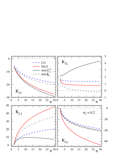
Figure 1: [color online] Physical anomalous dimensions $K_{AB}(n)$ in LO and NLO for $\{F_{A},F_{B}\}=\{F_{2},F_{L}/(a_{s}C_{L,q}^{(1)})\}$ assuming $\alpha_{s}=0.2$ and $n_{f}=3$. The dash-dotted and dotted lines, respectively, show the NLO results where all contributions from $C_{L,i}^{(2)}$ and $\beta_{0}$ to $K_{AB}^{(1)}$ in Eq. (15) have been omitted. A global factor of $a_{s}$ has been ignored in the perturbative expansion, i.e., $K_{AB}=K_{AB}^{(0)}+a_{s}K_{AB}^{(1)}+{\cal{O}}(a_{s}^{2})$ is displayed.

In Fig. 1 we illustrate the $n$ dependence of the LO and NLO singlet kernels $K_{AB}$ for the evolution of $\{F_{A},F_{B}\}=\{F_{2},F_{L}/(a_{s}C_{L,q}^{(1)})\}$ assuming $\alpha_{s}=0.2$ and $n_{f}=3$. As can be seen, NLO corrections are sizable for all singlet kernels, in particular, when compared with the perturbative expansion of the singlet splitting functions $P_{kl}(n)$ in (5); see Figs. 1 and 2 in Ref. ref:nnlo . This is, however, not too surprising given that the known large higher order QCD corrections to the Wilson coefficients $C_{L,g}$ and $C_{L,q}$ Moch:2004xu are absorbed into the physical anomalous dimensions $K_{AB}$ for the evolution of the DIS structure functions $F_{2}$ and $F_{L}$. The impact of contributions from the NLO coefficients $C_{L,g}^{(2)}$ and $C_{L,q}^{(2)}$ on the results obtained for $K_{AB}$ is illustrated by the dash-dotted lines in Fig. 1. Another source for large corrections are the terms proportional to $\beta_{0}$ in Eq. (15) as can be inferred from the dotted lines; note that $K_{L2}^{(1)}$ and $K_{LL}^{(1)}$ include terms proportional to $\beta_{0}C_{L,g}^{(2)}$ and $\beta_{0}C_{L,q}^{(2)}$. In Sec. III we will demonstrate how the differences between the LO and NLO kernels become apparent in the scale evolution of $F_{2,L}(x,Q^{2})$.

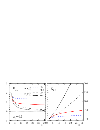
Figure 2: [color online] As in Fig. 1 but now comparing the LO and NLO off-diagonal kernels $K_{2L}$ and $K_{L2}$ for $\{F_{A},F_{B}\}=$ $\{F_{2},F_{L}/(a_{s}C_{L,q}^{(1)})\}$ and $\{F_{2},F_{L}/(a_{s}C_{L,g}^{(1)})\}$; see text.

Figure 2 compares the LO and NLO off-diagonal kernels $K_{2L}$ and $K_{L2}$ for $\{F_{A},F_{B}\}=$ $\{F_{2},F_{L}/(a_{s}C_{L,q}^{(1)})\}$ and $\{F_{2},F_{L}/(a_{s}C_{L,g}^{(1)})\}$. The most noticeable difference is the strong rise with $n$ for the kernel $K_{L2}$ governing the evolution of $\{F_{2},F_{L}/(a_{s}C_{L,g}^{(1)})\}$. At LO accuracy, this is readily understood by inspecting the $n\to\infty$ limit which yields, see Eq. (41) in Blumlein:2000wh , $K_{L2}^{(0)}\sim n\ln n$, recalling that asymptotically $C_{L,q}^{(1)}\sim 1/n$, $C_{L,g}^{(1)}\sim 1/n^{2}$, $P_{qq}^{(0)}\sim\ln n$, $P_{qg}^{(0)}\sim 1/n$, $P_{gq}^{(0)}\sim 1/n$, and $P_{gq}^{(0)}\sim\ln n$. The NLO kernel $K_{L2}$ exhibits an even stronger rise with $n$. In the same way one obtains, for instance, that $K_{L2}^{(0)}$ governing the evolution of $\{F_{2},F_{L}/(a_{s}C_{L,q}^{(1)})\}$ only grows like $\ln n$, see Eq. (13).

Despite this peculiar $n$ dependence and the differences between the singlet kernels shown in Fig. 2, both sets of observables, $\{F_{2},F_{L}/(a_{s}C_{L,q}^{(1)})\}$ and $\{F_{2},F_{L}/(a_{s}C_{L,g}^{(1)})\}$ can be used interchangeably in an analysis at LO and NLO accuracy. Results for the QCD scale evolution are identical, and one does not encounter any numerical instabilities related to the inverse Mellin transform, which we perform along a contour as described in Ref. Vogt:2004ns . In fact, it is easy to see that the eigenvalues

$$\lambda_{\pm}=\frac{1}{2}\left[K_{22}^{(0)}+K_{LL}^{(0)}\pm\sqrt{\!(K_{22}^{(0)}-K_{LL}^{(0)})^{2}\!+4K_{2L}^{(0)}K_{L2}^{(0)}}\,\right],$$ (17)

which appear when solving the matrix valued evolution equation (II.1), are identical for both sets of kernels and also agree with the corresponding eigenvalues for the matrix of singlet anomalous dimensions $P^{(0)}_{kl}$; see also the discussions in Sec. III

II.3 Example II: $F_{2}$ and $dF_{2}/dt$

Of future phenomenological interest could be also the pair of observables $\{F_{2},dF_{2}/dt\}$, in particular, in the absence of precise data for $F_{L}$. Determining experimentally the $t$ or $Q^{2}$ slope of $F_{2}$ is, of course, also challenging.

Defining $F_{D}\equiv dF_{2}/dt$, we obtain the following physical evolution kernels

$$K_{22}^{(0)} =0\,,\hskip 14.22636ptK_{2D}^{(0)}=2\,,$$

$$K_{D2}^{(0)} =\frac{1}{2}\left[P_{{gq}}^{(0)}P_{{qg}}^{(0)}-P_{{gg}}^{(0)}P_{{qq}}^{(0)}\right]\,,$$

$$K_{2D}^{{}^{(0)}} =P_{\text{gg}}^{(0)}+P_{\text{qq}}^{(0)}$$ (18)

at LO and

$$K_{22}^{(1)} =0\,,\hskip 14.22636ptK_{2D}^{(1)}=\frac{2\beta_{1}}{\beta_{0}}\,,$$

$$K_{D2}^{(1)} =\frac{1}{2}\bigg{\{}P_{{gq}}^{(1)}P_{{qg}}^{(0)}+P_{{gq}}^{(0)}P_{{qg}}^{(1)}-P_{{gg}}^{(1)}P_{{qq}}^{(0)}-P_{{gg}}^{(0)}P_{{qq}}^{(1)}$$

$$-\beta_{0}\bigg{(}P_{{qq}}^{(1)}+P_{{qg}}^{(1)}\frac{P_{{qq}}^{(0)}}{P_{{qg}}^{(0)}}\bigg{)}+\beta_{0}\bigg{[}-2C_{2,g}^{(1)}P_{{gq}}^{(0)}$$

$$+C_{{2q}}^{(1)}\bigg{(}P_{{qq}}^{(0)}+P_{{gg}}^{(0)}\bigg{)}+C_{2,g}^{(1)}\bigg{(}P_{{gg}}^{(0)}-P_{{qq}}^{(0)}\bigg{)}\frac{P_{{qq}}^{(0)}}{P_{{qg}}^{(0)}}\bigg{]}$$

$$+\beta_{0}^{2}\bigg{[}C_{2,q}^{(1)}-C_{\text{2g}}^{(1)}\frac{P_{{qq}}^{(0)}}{P_{{qg}}^{(0)}}\bigg{]}-\frac{\beta_{1}}{\beta_{0}}\bigg{[}P_{{gq}}^{(0)}P_{{qg}}^{(0)}-P_{{gg}}^{(0)}P_{{qq}}^{(0)}\bigg{]}\bigg{\}}\,,$$

$$K_{DD}^{(1)} =P_{{qq}}^{(1)}+P_{{gg}}^{(1)}-\beta_{0}\frac{1}{P_{{qg}}^{(0)}}P_{{qg}}^{(1)}+\beta_{1}$$

$$-2\beta_{0}C_{{2,q}}^{(1)}+\beta_{0}\frac{C_{{2,g}}^{(1)}}{P_{{qg}}^{(0)}}\bigg{(}P_{{qq}}^{(0)}-P_{{gg}}^{(0)}+\beta_{0}\bigg{)}\;,$$ (19)

at NLO accuracy to be used in Eq. (II.1). It is immediately obvious from Eq. (II.1) that $K_{22}=0$ to all orders. Likewise, $K_{2D}$ is also trivial and can be read off from $dF_{2}/d\ln Q^{2}=K_{2D}\,dF_{2}/dt$ order by order in $a_{s}$. After properly accounting for differences in the terms proportional to $\beta(a_{s})$, we agree with the results given in Blumlein:2000wh where the evolution equation (II.1) is expressed in terms of $d/dt$ rather than $d/d\ln Q^{2}$. The kernels $K_{AB}$ in (II.3) and (II.3) exhibit more moderate higher order corrections, mainly through terms proportional to $\beta_{0,1}$, than those listed in Sec. II.2. This shall become apparent in the next Section when we discuss results for the scale dependence of both $\{F_{2},dF_{2}/dt\}$ and $\{F_{2},F_{L}\}$.

III Numerical Studies

In this Section we apply the methodology based on physical anomalous dimensions as outlined above and compare with the results obtained in the conventional framework of scale-dependent quark and gluon densities and coefficient functions. Due to the lack of precise enough data for $F_{L}$ or $dF_{2}/dt$ we will adopt the following realistic “toy” initial conditions for the standard DGLAP evolution of PDFs at a scale $Q_{0}=\sqrt{2}\,\mathrm{GeV}$ Vogt:2004ns

$$xu_{v}(x,Q_{0}^{2}) =5.1072\,x^{0.8}\,(1-x)^{3},$$

$$xd_{v}(x,Q_{0}^{2}) =3.06432\,x^{0.8}\,(1-x)^{4},$$

$$x\bar{u}(x,Q_{0}^{2}) =(1-x)\,x\,\bar{d}(x,Q_{0}^{2}),$$

$$x\bar{d}(x,Q_{0}^{2}) =0.1939875\,x^{-0.1}\,(1-x)^{5},$$

$$x\bar{s}(x,Q_{0}^{2}) =0.2\,x\,[\bar{u}(x,Q_{0}^{2})+\bar{d}(x,Q_{0}^{2})],$$

$$xg(x,Q_{0}^{2}) =1.7\,x^{-0.1}\,(1-x)^{5}.$$ (20)

for all our numerical studies. The value of the strong coupling $\alpha_{s}$ at $Q_{0}$ is taken to be $0.35$. For our purposes we can ignore the complications due to heavy flavor thresholds and set $n_{f}=3$ throughout. We use this set of PDFs to compute the flavor singlet parts of $F_{2}$, $F_{L}$, and $dF_{2}/dt$ at the input scale $Q_{0}$ using Eq. (10). For studies of DIS in the small $x$ region, say $x\lesssim 10^{-3}$, in which we are mainly interested in, the flavor singlet parts are expected to dominate over NS contributions and, hence, shall be a good proxy for the full DIS structure functions. Results at scales $Q>Q_{0}$ are obtained by either solving the RGEs for PDFs or by evolving the input structure functions directly adopting Eq. (II.1). For the solution in terms of PDFs we adopt from now on the standard choice $\mu=Q$.

For completeness and to facilitate the discussions below, let us quickly review the solution of the matrix-valued RGEs such as Eqs. (4) and (II.1). While one can truncate the QCD beta function and the anomalous dimensions consistently at any given order in $a_{s}$, there exists no unique solution to (II.1) beyond the LO accuracy. The matrix-valued nature of (II.1) only allows for iterations around the LO solution, which at order $a_{s}^{k}$ can differ in various ways by formally higher-order terms of ${\cal{O}}(a_{s}^{l>k})$.

To this end, we employ the standard truncated solution in Mellin moment space, which can be found, for instance, in Ref. Gluck:1989ze , see also Vogt:2004ns , and reads

$$\Gamma_{i}(n,Q) =L_{i}(n,a_{s},a_{0})\Gamma_{i}(n,Q_{0})$$ (21)

where the evolution operator up to NLO is defined as

$$L_{i}(n,a_{s},a_{0}) =L^{(0)}_{i}(n,a_{s},a_{0})+L^{(1)}_{i}(n,a_{s},a_{0})$$ (22)

with

$$L^{(0)}_{i}(n,a_{s},a_{0}) =\left(\frac{a_{s}}{a_{0}}\right)^{-\frac{\lambda_{-}}{\beta_{0}}}e_{-}+(+)\leftrightarrow(-)$$

$$L^{(1)}_{i}(n,a_{s},a_{0}) =\left(\frac{a_{s}}{a_{0}}\right)^{-\frac{\lambda_{-}}{\beta_{0}}}\Bigg{[}(a_{0}-a_{s})e_{-}R_{i}^{(1)}e_{-}$$

$$-\left(a_{0}-a_{s}\left(\frac{a_{s}}{a_{0}}\right)^{\frac{\lambda_{-}-\lambda_{+}}{\beta_{0}}}\right)\beta_{0}\frac{e_{-}R_{i}^{(1)}e_{+}}{\lambda_{+}-\lambda_{-}-\beta_{0}}\Bigg{]}$$

$$\qquad+\quad(+)\leftrightarrow(-)\;.$$ (23)

Here, $a_{0}=a_{s}(Q_{0})$, $\Gamma_{P}=\left(\Sigma\atop g\right)$, and $\Gamma_{K}=\left(F_{A}\atop F_{B}\right)$, i.e., the index $i=P$ refers to the coupled RGE for the quark singlet and gluon and $i=K$ to the RGE for the pair $\{F_{A},F_{B}\}$ of DIS structure functions in (II.1). For $i=K$ one has

$$\left(R_{K}^{(0)}\right)_{AB}=\frac{1}{\beta_{0}}K_{AB}^{(0)}\;\;,\;\;\left(R_{K}^{(1)}\right)_{AB}=\frac{1}{\beta_{0}}K_{AB}^{(1)}-\frac{\beta_{1}}{\beta_{0}^{2}}K_{AB}^{(0)}\,,$$ (24)

with a corresponding definition for $i=P$ in terms of the $2\times 2$ matrices of singlet splitting functions $P^{(0)}$ and $P^{(1)}$. $\lambda_{\pm}$ denote the eigenvalues given in Eq. (17) and $e_{\pm}$ the projection operators onto the corresponding eigenspaces; see Refs. Gluck:1989ze ; Vogt:2004ns .

As has been mentioned already at the end of Sec. II.2, the eigenvalues $\lambda_{\pm}(n)$ are identical when computed for the kernels $K_{AB}$ and $P_{kl}$. This in turn implies that as long as, say, $F_{2}$ and $F_{L}$ are calculated at $\mu=Q_{0}$ with LO accuracy, their scale evolution based on physical anomalous dimensions reproduces exactly the conventional results obtained with the help of scale-dependent PDFs.

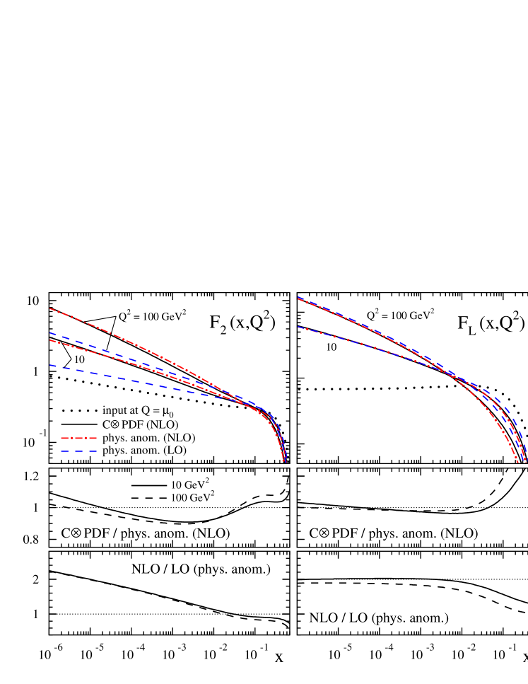
Figure 3: [color online] Scale dependence of the DIS structure functions $F_{2}$ (left) and $F_{L}$ (right) at NLO accuracy obtained with physical anomalous dimensions (dash-dotted lines) and in the standard way through a convolution of PDFs and Wilson coefficients (solid lines). The dashed and dotted lines show the results obtained at LO accurary and the input at $Q=Q_{0}=\sqrt{2}\,\mathrm{GeV}$, respectively. The middle panels give the ratios of the two different methods to evolve $F_{2,L}$ at NLO, and the lower panels illustrate the size of NLO corrections when physical anomalous dimensions are being used; see text.

Figure 3 shows our results for the scale dependence of the DIS structure functions $F_{2}$ and $F_{L}$. The input functions at $Q_{0}=\sqrt{2}\,\mathrm{GeV}$ are shown as dotted lines. While LO results are identical, starting from NLO accuracy the comparison between the two methods of scale evolution becomes more subtle, and results seemingly differ significantly as can be inferred from the middle panels of Fig. 3.

The origin of the differences between $F_{2,L}(x,Q^{2})$ computed based on Wilson coefficients and scale-dependent PDFs and physical anomalous dimensions can be readily understood from terms which are formally beyond NLO accuracy. For instance, upon inserting the NLO Wilson coefficients (3) and the truncated NLO solution (21)-(III) into Eq. (10), $F_{2}$ at ${\cal{O}}(a_{s})$ contains spurious terms of both ${\cal{O}}(a_{0}a_{s})$ and ${\cal{O}}(a_{s}^{2})$. Since $F_{L}$ starts one order higher in $a_{s}$, similar terms are less important here. On the other hand, when we evolve $F_{2,L}$ with the help of physical anomalous dimensions we first compute, due to the lack of data, the input at $a_{0}$ based on Eq. (10), which then enters the RGE solution (21)-(III). Again, this leads to terms beyond NLO. In case of $F_{2}$ they are now of the order ${\cal{O}}(a_{0}a_{s})$ and ${\cal{O}}(a_{0}^{2})$, i.e., even more relevant than in case of PDFs since $a_{0}>a_{s}$.

To test if the entire difference between the two evolution methods shown in Fig. 3 is caused by these spurious higher order contributions, one can easily remove all ${\cal{O}}(a_{s}^{2})$, ${\cal{O}}(a_{0}a_{s})$, and ${\cal{O}}(a_{0}^{2})$ contributions from our results. Indeed, the scale evolution based on physical anomalous dimensions and the calculation of $F_{2,L}$ from PDFs then yields exactly the same results also at NLO accuracy. We note that this way of computing properly truncated physical observables from scale-dependent PDFs beyond the LO accuracy has been put forward some time ago in Refs. Gluck:1983bh ; Gluck:1991jc but was not pursued any further in practical calculations.

Another interesting aspect to notice from Fig. 3 are the sizable NLO corrections illustrated in the lower panels, in particular, for $F_{2}$ in the small $x$ region. For this comparison, LO results refer to the same input structure functions $F_{2,L}$ as used to obtain the NLO results but now evolved at LO accuracy, i.e., by truncating the evolution operator in Eqs. (21)-(III) at $L_{K}^{(0)}$. At first sight the large corrections appear to be surprising given that global PDF fits in general lead to acceptable fits of DIS data even at LO accuracy ref:pdffits . However, this is usually achieved by exploiting the freedom of having different sets of PDFs at LO and, say, NLO accuracy to absorb QCD corrections. The framework based on physical anomalous dimensions does not provide this option as the input for the scale evolution is, in principle, fully determined by experimental data, and only the value for the strong coupling can be adjusted at any given order. In this sense it provides a much more stringent test of the underlying framework and perhaps a better sensitivity to, for instance, the possible presence of non-linear effects to the scale evolution in the kinematic regime dominated by small $x$ gluons.

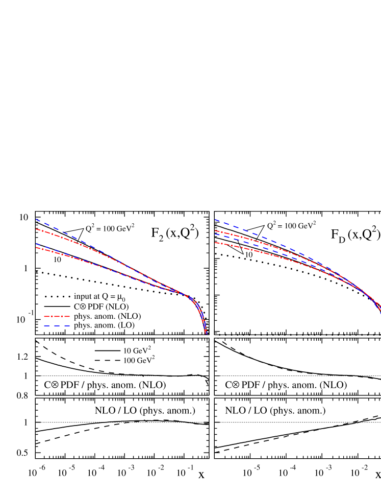
Figure 4: [color online] Same as in Fig. 4 but now for the pair of observables $F_{2}$ and $F_{D}\equiv dF_{2}/dt$.

In Fig. 4 we show the corresponding results for the scale dependence of the DIS structure function $F_{2}$ and its slope $F_{D}=dF_{2}/dt$. Again, any differences between the scale evolution performed with physical anomalous dimensions and based on PDFs are caused by formally higher order terms ${\cal{O}}(a_{s}^{2})$, ${\cal{O}}(a_{0}a_{s})$, and ${\cal{O}}(a_{0}^{2})$, which can be removed with the same recipe as above. As for $\{F_{2},F_{L}\}$, NLO corrections are sizable in the small $x$ region due to numerically large contributions to $K^{(1)}_{D2}$ and $K^{(1)}_{DD}$ from the QCD beta function.

We close our discussions by noting that NLO corrections to the NS RGEs are much more moderate than in the singlet sector. This also holds for the importance of spurious higher order terms discussed above. Hence, we refrain from showing any numerical results here. We also wish to recall that we have ignored for our purposes any complications in the scale evolution due heavy quark flavors by setting $n_{f}=3$ throughout. While heavy quarks of mass $m_{h}$ can be straightforwardly included above a scale $Q=m_{h}$ in a massless approximation by introducing a new NS combination, which is properly matched to the singlet part at $Q=m_{h}$, more sophisticated treatments require work beyond the scope of this work. For instance, if heavy quark contributions to DIS structure functions are treated with their full mass and threshold dependence, and without resumming any potentially large logarithms $\log(Q/m_{h})$ Gluck:1993dpa , one can compute another set of physical anomalous dimensions for, say, the pair of observables $\{F_{2}^{h},F_{L}^{h}\}$, based on the appropriate fully massive NLO Wilson coefficients in Ref. Laenen:1992zk .

IV Summary

We have presented a phenomenological study of the QCD scale evolution of deep-inelastic structure functions within the framework of physical anomalous dimensions. The method is free of ambiguities from choosing a specific factorization scheme and scale as it does not require the introduction of parton distribution functions. Explicit results for the physical evolution kernels needed to evolve the structure functions $F_{2}$, its $Q^{2}$ slope, and $F_{L}$ have been presented up to next-to-leading order accuracy.

It was shown that any differences with results obtained in the conventional framework of scale-dependent quark and gluon densities can be attributed to the truncation of the perturbative series at a given order in the strong coupling. At next-to-leading order accuracy the numerical impact of these formally higher order terms is far from being negligible but, if desired, such contributions can be systematically removed.

A particular strength of performing the QCD scale evolution based on physical anomalous dimensions rather than using auxiliary quantities such as parton densities is that the required initial conditions are completely fixed by data and cannot be tuned freely in each order of perturbation theory. Apart from a possible adjustment of the strong coupling, this leads to easily testable predictions for the scale dependence of structure functions and also clearly exposes the relevance of higher order QCD corrections in describing deep-inelastic scattering data. Next-to-leading order corrections have been demonstrated to be numerically sizable, which is not too surprising given that the physical evolution kernels absorb all known large higher order QCD corrections to the hard scattering Wilson coefficients.

Once high precision deep-inelastic scattering data from future electron-ion colliders become available, an interesting application of our results will be to unambiguously quantify the size and relevance of non-linear saturation effects caused by an abundance of gluons with small momentum fractions. To this end, one needs to observe deviations from the scale evolution governed by the physical anomalous dimensions discussed in this work. The method of physical anomalous dimensions can be also used for a theoretically clean extraction of the strong coupling and is readily generalized to other processes such polarized deep-inelastic scattering or inclusive one-hadron production.

References

- (1) For recent PDF analyses, see: H. -L. Lai et al., Phys. Rev. D 82, 074024 (2010); J. Gao et al., arXiv:1302.6246 [hep-ph]; A. D. Martin, W. J. Stirling, R. S. Thorne, and G. Watt, Eur. Phys. J. C 63, 189 (2009); R. D. Ball et al. [The NNPDF Collaboration], Nucl. Phys. B 874, 36 (2013); S. Alekhin, J. Blumlein, S. Klein, and S. Moch, Phys. Rev. D 81, 014032 (2010).
- (2) F. D. Aaron et al. [H1 and ZEUS Collaboration], JHEP 1001, 109 (2010).
- (3) See, e.g., J. C. Collins, D. E. Soper, and G. F. Sterman, Adv. Ser. Direct. High Energy Phys. 5, 1 (1988).
- (4) W. Furmanski and R. Petronzio, Z. Phys. C 11, 293 (1982).
- (5) W. L. van Neerven and E. B. Zijlstra, Phys. Lett. B 272, 127 (1991); Phys. Lett. B 273, 476 (1991); Nucl. Phys. B 383, 525 (1992).
- (6) S. Moch and J. A. M. Vermaseren, Nucl. Phys. B 573, 853 (2000).
- (7) D. I. Kazakov and A. V. Kotikov, Nucl. Phys. B 307, 721 (1988) [Erratum-ibid. B 345, 299 (1990)]; D. I. Kazakov, A. V. Kotikov, G. Parente, O. A. Sampayo, and J. Sanchez Guillen, Phys. Rev. Lett. 65, 1535 (1990) [Erratum-ibid. 65, 2921 (1990)]; J. Sanchez Guillen, J. Miramontes, M. Miramontes, G. Parente, and O. A. Sampayo, Nucl. Phys. B 353, 337 (1991).
- (8) For a recent review on DIS, see, e.g., J. Blumlein, Prog. Part. Nucl. Phys. 69, 28 (2013).
- (9) D. J. Gross and F. Wilczek, Phys. Rev. D 9, 980 (1974); H. Georgi and H. D. Politzer, Phys. Rev. D 9, 416 (1974); V. N. Gribov and L. N. Lipatov, Sov. J. Nucl. Phys. 15, 438 (1972) [Yad. Fiz. 15, 781 (1972)]; G. Altarelli and G. Parisi, Nucl. Phys. B 126, 298 (1977); Y. L. Dokshitzer, Sov. Phys. JETP 46, 641 (1977) [Zh. Eksp. Teor. Fiz. 73, 1216 (1977)]; K. J. Kim and K. Schilcher, Phys. Rev. D 17, 2800 (1978).
- (10) E. G. Floratos, D. A. Ross, and C. T. Sachrajda, Nucl. Phys. B 129, 66 (1977) [Erratum-ibid. B 139, 545 (1978)]; G. Curci, W. Furmanski, and R. Petronzio, Nucl. Phys. B 175, 27 (1980); W. Furmanski and R. Petronzio, Phys. Lett. B 97, 437 (1980); A. Gonzalez-Arroyo, C. Lopez, and F. J. Yndurain, Nucl. Phys. B 153, 161 (1979); A. Gonzalez-Arroyo and C. Lopez, Nucl. Phys. B 166, 429 (1980); E. G. Floratos, R. Lacaze, and C. Kounnas, Phys. Lett. B 98, 89 (1981); Phys. Lett. B 98, 285 (1981); Nucl. Phys. B 192, 417 (1981).
- (11) S. Moch, J. A. M. Vermaseren, and A. Vogt, Nucl. Phys. B 688, 101 (2004); Nucl. Phys. B 691, 129 (2004).
- (12) W. A. Bardeen, A. J. Buras, D. W. Duke, and T. Muta, Phys. Rev. D 18, 3998 (1978).
- (13) S. Catani, Z. Phys. C 75, 665 (1997).
- (14) J. Blumlein, V. Ravindran, and W. L. van Neerven, Nucl. Phys. B 586, 349 (2000).
- (15) G. Soar, S. Moch, J. A. M. Vermaseren, and A. Vogt, Nucl. Phys. B 832, 152 (2010).
- (16) D. Boer et al., arXiv:1108.1713 [nucl-th]; A. Accardi et al., arXiv:1212.1701 [nucl-ex].
- (17) J. L. Abelleira Fernandez et al., arXiv:1211.4831 [hep-ex].
- (18) J. Blumlein and H. Bottcher, Nucl. Phys. B 636, 225 (2002). [hep-ph/0203155].
- (19) E. C. Aschenauer, R. Sassot, and M. Stratmann, Phys. Rev. D 86, 054020 (2012); E. C. Aschenauer, T. Burton, T. Martini, H. Spiesberger, and M. Stratmann, arXiv:1309.5327.
- (20) See, e.g., D. de Florian, R. Sassot, and M. Stratmann, Phys. Rev. D 75, 114010 (2007).
- (21) A. Vogt, Comput. Phys. Commun. 170, 65 (2005).
- (22) M. Gluck, E. Reya, and A. Vogt, Z. Phys. C 48, 471 (1990).
- (23) J. Blumlein, Comput. Phys. Commun. 133, 76 (2000).
- (24) J. Blumlein and S. Kurth, Phys. Rev. D 60, 014018 (1999).
- (25) S. Moch, J. A. M. Vermaseren and A. Vogt, Phys. Lett. B 606, 123 (2005) [hep-ph/0411112].
- (26) M. Gluck, K. Grassie, and E. Reya, Phys. Rev. D 30, 1447 (1984).
- (27) M. Gluck, E. Reya, and A. Vogt, Phys. Rev. D 46, 1973 (1992).
- (28) See, for instance, M. Gluck, E. Reya, and M. Stratmann, Nucl. Phys. B 422, 37 (1994) and references therein.
- (29) E. Laenen, S. Riemersma, J. Smith, and W. L. van Neerven, Nucl. Phys. B 392, 162 (1993).