The Polyakov loop in various representations in the confined phase of QCD

Abstract

We analyze the expectation value of the Polyakov loop in the fundamental and higher representations in the confined phase of QCD. We discuss a hadronic like representation, and find that the Polyakov loop corresponds to a partition function in the presence of a colored source, explaining its real and positive character. Saturating the sum rules to intermediate temperatures requires a large number of multipartonic excited states. By using constituent or bag models, we find detailed low temperature scaling rules which depart from the Casimir scaling and could be tested by lattice calculations.

I Introduction

The thermodynamics of ${\mathrm{SU}}(N_{c})$ non Abelian gauge theories with or without matter Dirac fields with $N_{f}$ flavors has received much attention and interest due to a possible realization of new phases at sufficiently high temperatures such as the quark-gluon plasma Shuryak (1978); Meyer-Ortmanns (1996). This is relevant in the early stages of the universe or in the laboratory at accelerator facilities such as SPS, RHIC and LHC Harris and Muller (1996); Meyer-Ortmanns (1996); Muller and Nagle (2006); Fukushima (2012). Indeed, the initial and unique pioneering Quantum Chromodynamics (QCD) predictions of lattice QCD Kogut et al. (1983); Polonyi et al. (1984); Pisarski and Wilczek (1984), now firmly established  Aoki et al. (2006); Bazavov et al. (2012), of a phase transition provided a strong motivation to search for the quark-gluon plasma phase in the Laboratory. The phase transition from a confined and chirally spontaneous broken phase to a deconfined and chirally symmetric phase is characterized by a steep change of the chiral condensate $\langle\bar{q}q\rangle$ and the Polyakov loop expectation values. Actually, they become true order parameters in the limits of massless and infinitely heavy quarks respectively. In the real world the transition temperature is defined as the inflexion point of both observables. Both the quark condensate and the Polyakov loop require a (multiplicative) renormalization and hence demand a delicate analysis on the lattice.

Because of these promising expectations, and also because lattice calculations become more difficult at finite but small temperatures, the phase transition picture has naturally and traditionally dominated theoretical approaches and insightful guesswork in the past. These include effective potential methods Megias et al. (2004); Braun et al. (2010, 2011); Smith et al. (2013), and quark models Meisinger and Ogilvie (1996); Fukushima (2004). Hence, the focus of studies and model building was placed on the understanding of the physics around the phase transition with less attention on the low temperature range and its detailed features.

On the other hand, a long term scrutiny over the last 30 years has culminated revealing a by now widely accepted cross-over Aoki et al. (2006) (for a review see e.g. Fodor (2012)), at about a temperature of $T\approx 200{\rm MeV}$ indicating the co-existence of hadronic and quark-gluon degrees of freedom. To our knowledge, the physical mechanism how this cross-over starts to manifest itself remains unclear (see however Jakovac (2013)).

This turn of the subject suggests that we may actually improve our theoretical understanding by looking into the pre-deconfinement regime in terms of hadronic degrees of freedom. At very low temperature, the low lying and well known hadronic states will dominate any physical observable, as they will effectively behave as elementary and stable states, so that their multipartonic nature will not show up. This effective elementarity is buttressed by the quantum virial expansion among hadrons (including unstable resonances) Dashen et al. (1969); Dashen and Rajaraman (1974) and provides the basis of the Hadron Resonance Gas (HRG) model. Through the assumption of completeness of hadronic states the HRG model implements the quark-hadron duality at finite temperature as a multicomponent gas of non-interacting massive stable and point-like particles Hagedorn (1985). Such a simple model has been used as a reference to compare with lattice calculations of the trace anomaly and the quark condensate at low temperature, particularly because of initially unsettled discrepancies, which finally came to an agreement among themselves and with the HRG model Karsch et al. (2003); Borsanyi et al. (2010a); Huovinen and Petreczky (2010); Borsanyi et al. (2013). Remarkably, the disagreement still persists beyond the expected range of validity of the HRG model. Although this gives the HRG model a distinct arbitrating role, its validity based on microscopic arguments has only been checked in the strong coupling limit and for heavy quarks to lowest orders Langelage and Philipsen (2010) or in chiral quark models under very specific assumptions Ruiz Arriola et al. (2013a); Megias et al. (2013a, b). Recent applications of the HRG model include also the study of QCD transport coefficients Noronha-Hostler et al. (2012), QCD in presence of small magnetic fields Endrödi (2013); Bali et al. (2013), and nucleus-nucleus collisions at relativistic energies Cleymans and Redlich (1999); Begun et al. (2013).

The HRG model requires using specific hadronic states, and those listed in the PDG booklet Beringer et al. (2012) provide the standard ones in computations of the trace anomaly for light flavors. These calculations exclude the exotic states on the HRG model side, although high accuracy would be needed anyhow in order to discriminate if they are to be seen distinctly in lattice calculations. One must in addition make an assessment on the error of the HRG model itself. The simple half width rule error estimate of Ref. Arriola et al. (2013) based on the resonance character of most excited states suggests that both lattice and the HRG model already agree within their uncertainties. Thus, we do not view finite temperature calculations of the trace anomaly as a viable way of unveiling the, so far, scarce exotic states.

In a recent paper Megias et al. (2012) we have established a hadronic representation of the Polyakov loop in the fundamental representation, a purely gluonic but gauge invariant and hence color singlet operator, which corresponds to the QCD partition function in the presence of a color triplet fixed source. For the usual light $u,d,s$ quarks the low lying part of the spectrum of such a theory can be approximated by mesons and baryons with just one heavy quark, either $c$ or $b$. This partition function character guarantees the positivity and monotonicity of the Polyakov loop expectation value at low temperatures, a fact which is not obvious by other means but has always been observed in lattice calculations . In our view, these observations make, despite traditional reservations, the renormalized Polyakov loop an observable in much the same way as the renormalized chiral condensate.

The situation and prospectives for the Polyakov loop in the fundamental representation are rather different as compared to the trace anomaly or the quark condensate for light $u,d,s$ quarks. Firstly, there are much less listed PDG states with one additional $c$ or $b$ quark. Thus, in order to saturate the hadronic representation one would need rather small temperatures, which by the leading exponential Boltzmann suppression would provide too weak a signal in lattice calculations. However, at current available temperatures two different lattice groups agree on this observable Bazavov et al. (2012); Borsanyi et al. (2010b) so its analysis may be more robust. Besides, the renormalized Polyakov loop turns out to be approximately bound by the number of colors , which sets a necessary validity range for the HRG model calculation. As we will show, the presence of exotic states becomes very visible still within the range where we expect the HRG model to work.

A recent lattice calculation has explicitly implemented the sum rule for the Polyakov loop we have derived in a previous work Megias et al. (2012) using a finite number of excited lattice QCD states Bazavov and Petreczky (2013) although large uncertainties are displayed for $T\geq 140{\rm MeV}$. The origin of the uncertainties is intriguing, and no clear conclusions regarding the existence of exotic states have been reached.

In any case, as the temperature is raised there will be manifest quark and gluon exchange effects which we will discuss in some detail. Our analysis will face, once more, the difficulties in making a clear cut definition of a hadronic state out of multiparton states. We note incidentally, that all established states listed in the PDG have a $\bar{q}q$ and $qqq$ assignment in the quark model, with no missing states but further states. This implies that in the confining regime we expect the hadronic basis of states to be complete.

As mentioned above, most works on finite temperature have been stimulated by the occurrence of the phase-transition. However, even if a rapid change of order parameters takes place at some critical temperature, the proper low temperature behavior is not guaranteed. A prominent example is provided by chiral quark models at finite temperature, which have been massively used and reproduced a chiral phase transition in spite of violating low temperature requirements, such as the $1/N_{c}$ suppression of finite temperature corrections as well as chiral perturbation theory requirements (see e.g. for a thorough discussion Megias et al. (2006a, b)). In quark models the situation was mended by including the Polyakov loop variable Meisinger and Ogilvie (1996), which has generated a wealth of publications Fukushima (2004); Megias et al. (2006a, b); Ratti et al. (2006); Sasaki et al. (2007); Ciminale et al. (2008); Contrera et al. (2008); Schaefer et al. (2007); Ghosh et al. (2008); Costa et al. (2009); Mao et al. (2010); Sakai et al. (2010); Radzhabov et al. (2011); Zhang et al. (2010). However, in most implementations of the Polyakov loop Nambu–Jona-Lasinio (PNJL) model, a plain mean-field approximation is applied, the goal being to describe the interplay between the breaking of chiral and center symmetries and features of the QCD phase diagram. Unfortunately such mean-field approximation erases detailed information such as the Polyakov loop expectation values in higher representations. In a recent communication we have shown that the quantum and local nature of the Polyakov loop Megias et al. (2007a); Ruiz Arriola et al. (2013a) becomes indispensable in order to make contact with the HRG model both for the partition function as well as for the Polyakov loop as deduced in Ref. Megias et al. (2012). Thus, there is at present no model where i) the HRG model is reproduced at low temperatures and ii) the confinement-chiral crossover transition observed on the lattice is reproduced Ruiz Arriola et al. (2013a); Megias et al. (2013c); Ruiz Arriola et al. (2013b). In the present paper we focus on features at low temperatures, leaving possible extensions for the deconfined phase for future work. While at this level of description we are only confronted with rather global aspects of hadrons we already face ambiguities regarding color singlet clustering inside a global color singlet state.

Ideally the sum rule for the Polyakov loop would be saturated by just using accepted PDG states with $c,b$ as heavy quarks and $u,d,s$ as light quarks. However, unlike the $u,d,s$ spectrum there are much less $c,b$ states. For this reason in Ref. Megias et al. (2012) we saturated the sum rule for the Polyakov loop using quark model spectra for $\bar{q}Q$ and $qqQ$ color singlet states with one heavy $Q=c,b$ quark and the remaining light quarks $q=u,d,s$. While heavy quarks exhibit their non-relativistic nature for the low lying states, the fact that many excited states were needed suggested using relativistic kinematics as the one of the Relativized Quark Model (RQM) Godfrey and Isgur (1985); Capstick and Isgur (1986). Unfortunately, going beyond three-particle systems, i.e. tetraquark, hybrids or pentaquark excited states within the RQM requires assumptions about the color structure of interactions. There is a wealth of work on multiquark systems (see e.g.Ref. Richard (2010) for a lucid summary and references therein) but we consider that despite much progress in recent times in quark models Vijande et al. (2007), QCD sum rules Nielsen et al. (2010) or lattice QCD, the theory is not on a satisfactory state as to make unambiguous predictions on what states should one consider into the partition function at finite temperatures. Therefore, and following our previous work, we will analyze independent particle models, such as the MIT bag model and PNJL models where the problem reduces to evaluating degeneracies of singlet multiquark and multigluon states, which will be refereed to as multiparton states for short.

However, even if a sufficient number of PDG states were available there still remains the problem on what states should be used. This brings us to the issue of completeness of the hadronic spectrum. There are currently no redundancy of states in the PDG as compared to the quark model assignment. For instance, the concerns on the proliferation of the new $X,Y,Z$ states poses a serious theoretical question which have been spelled out Carames et al. (2012) and can be traced to the identification of states in terms of constituents. One of the advantages of our approach is that the correct counting of singlet multiparton states is guaranteed, and the discussion on under– or over– completeness of states is shifted to the concept of singlet cluster irreducibility and the corresponding effective elementarity Rajaraman (1979).

The generalization of the previous discussion to other representations besides the fundamental one is straightforward, and in the present paper we want to analyze the Polyakov loop in the lowest higher representations. Unfortunately, the extraction of the spectrum from hadronic systems seems even less obvious so we will provide some initial estimates by using specific models with quark and gluon degrees of freedom.

For instance, if the color source is in the adjoint representation we may imagine that it corresponds to a heavy gluon or two heavy quarks coupled adjointwise. Heavy quarks exhibit their non-relativistic nature for the low lying hadronic states. However, we expect important relativistic corrections in the higher part of the energy spectrum. Thus, the models that we will be using embody relativistic kinematics for the light degrees of freedom.

Casimir scaling is one of the features which is suggested by lowest orders in perturbation theory in QCD and still holds non-perturbatively on the lattice numerically . The most studied example is given by the string tension. This scaling has been advocated in Ref. Gupta et al. (2008) within the study of renormalized Polyakov loops in many representations. Casimir scaling has also been observed on the lattice Mykkanen et al. (2012) in pure ${\mathrm{SU}}(N_{c})$ gauge theories at several values of $N_{c}$ above the phase transition for the renormalized Polyakov loop. In the present paper we provide alternative scaling patterns which differ from the Casimir scaling ones and apply at low temperatures below the phase transition.

QCD is characterized among other things by quark-gluon confinement of the physically observable hadronic states, which exhibit a finite energy gap with the vacuum. For non strange hadrons there are two main gaps: $m_{\pi}$ and $m_{\rho}$. This allows for a clear separation at low temperatures where thermal effects are just due to a pion gas in a defined temperature range. Beyond these gaps, hadron states start to pile up with large multiplicities, eventually suggesting a Hagedorn spectrum which is not manifested in the thermodynamics of QCD. Thus, we expect that by looking into violations of quark-hadron duality at finite temperature, we may learn about the mysterious mechanisms of deconfinement at the lowest possible temperatures. As a general rule we find an expansion in the number of constituents a suitable tool to discriminate the effective elementarity of hadrons at low temperatures.

The manuscript is organized as follows. In Sec. II we introduce the hadron resonance gas model for the Polyakov loop based on generic QCD arguments. We apply this formalism in Sec. III within an independent multiparticle picture, and state the basis of the expansion in the number of constituents. These results will be applied later in concrete models, in particular the Polyakov constituent quark model in Sec. IV, and the bag model in Secs. V and VI. We present in Sec. VII some low temperature scaling relations of the Polyakov loop. Finally we conclude with a discussion of our results and an outlook towards possible future directions in Sec. VIII. Some technical details and further numerical results for the bag model are collected in the appendices.

II Hadron resonance gas model for the Polyakov loop

In this section we elaborate on the derivation of the sum rule for the Polyakov loop in a general irreducible representation of the color ${\mathrm{SU}}(N_{c})$ gauge group in terms of singlet hadronic states. Also $N_{c}$ is kept arbitrary here.

II.1 The Polyakov loop and the hadron resonance gas

Let $\cal{H}$ denote the Hilbert space of all possible configurations of (dynamical) quarks, antiquarks and gluons. As is known in gauge theories, the functional integration over $A_{0}$ takes care of projecting onto the physical subspace of states which are color singlet at every point ${\bm{x}}$, $\cal{H}_{\rm singlet}\subset\cal{H}$. That is, the QCD partition function (we do not include a chemical potential in this work) is

$$Z_{\rm QCD}={\rm Tr}_{\cal{H}_{\rm singlet}}(e^{-\beta H_{\rm QCD}})={\rm Tr}_{\cal{H}}(e^{-\beta H_{\rm QCD}}P_{\cal{H}_{\rm singlet}}),$$ (1)

where $H_{\rm QCD}$ denotes the QCD Hamiltonian, $\beta=1/T$ is the inverse temperature and

$$P_{\cal{H}_{\rm singlet}}=\int\prod_{{\bm{x}}}U(\Omega({\bm{x}}))d\Omega({\bm{x}}),$$ (2)

is the projector onto $\cal{H}_{\rm singlet}$, the space that contains the physical states made of quarks, antiquarks and gluons. Here $U(\Omega)$ is the unitary operator representing the element $\Omega$ of ${\mathrm{SU}}(N_{c})$ acting on the fields at given point, and $d\Omega$ is the ${\mathrm{SU}}(N_{c})$ Haar measure.

Other subspaces of $\cal{H}$ can be explored by introducing static color charges at different points. Specifically, the subspace which is in the antifundamental representation at ${\bm{x}}_{0}$ and singlet everywhere else, can be investigated by adding a fundamental source at ${\bm{x}}_{0}$, such as an infinitely heavy quark sitting at that point. The source polarizes the system since dynamical quarks, antiquarks, and gluons collaborate to neutralize the source in order to have a color singlet everywhere. In the confining phase the polarization takes place through nearby dynamical particles which screen the source at distance $r\sim T/\sigma$, where $\sigma$ is the string tension. Other irreducible representations (irreps) of ${\mathrm{SU}}(N_{c})$ can be considered as well by using different color sources, e.g., by adding the appropriate combination of heavy quarks and/or antiquarks to form the given representation. Note that the color sources represent heavy enough particles so that they can be given a well-defined position, are at rest and have no other active degree of freedom apart from color (even the spin and flavor states of the source can be disregarded due to heavy-quark symmetry).

Mathematically, the projector on a given irrep $\mu$ can be written as Tung (1985)

$$P_{\mu}=n_{\mu}\int\chi_{\mu}(\Omega^{-1})\,U(\Omega)\,d\Omega$$ (3)

where $n_{\mu}$ denotes the dimension of the representation, $\chi_{\mu}(\Omega)$ denotes the character of the element $\Omega$ in the irrep $\mu$, i.e., the trace of $U(\Omega)$ when $U$ falls in that irrep. Therefore, the QCD partition function when a color charge in the irrep $\mu$ is sitting at ${\bm{x}}_{0}$ would be

$$Z_{{\rm QCD},\mu}={\rm Tr}_{\cal{H}}\left[e^{-\beta H_{\rm QCD}}\int\chi_{\mu}(\Omega({\bm{x}}_{0}))\prod_{{\bm{x}}}U(\Omega({\bm{x}}))\,d\Omega({\bm{x}})\right].$$ (4)

Note (i) that our convention is to call $\mu$ to the irrep of the static source, and so the polarized system of dynamical quarks, antiquarks and gluons itself is in the conjugate irrep $\bar{\mu}$ at ${\bm{x}}_{0}$ (and in color singlet at any other point). So we have applied $P_{\bar{\mu}}$, and used $\chi_{\bar{\mu}}(\Omega^{-1})=\chi_{\mu}(\Omega)$, with $\Omega=\Omega({\bm{x}}_{0})$ in Eq. (3). And (ii), $Z_{{\rm QCD},\mu}$ is actually the partition function divided by $n_{\mu}$. Just one of the $n_{\mu}$ color-degenerated states is counted. This counting is automatically obtained by the coupling of the heavy source and the dynamical system to form a color singlet Luscher and Weisz (2002); Jahn and Philipsen (2004). The (infinite) mass of the source is excluded from the partition function.

In the Euclidean formulation of the gauge theory, the local gauge rotation $\Omega$ is realized by the Polyakov loop, i.e., the gauge covariant operator defined as

$$\Omega({\bm{x}})=P\,e^{\,i\int_{0}^{\beta}A_{0}(x)\,dx_{0}},$$ (5)

where $P$ indicates path ordering and $A_{0}$ and $x$ are Euclidean. Thus Eq. (4) can be rewritten as the ratio of two partition functions, to match the usual definition of expectation value of the Polyakov loop in the irrep $\mu$:

$$L_{{\rm QCD},\mu}(T):=\langle\chi_{\mu}(\Omega)\rangle_{\rm QCD}=\frac{Z_{{\rm QCD},\mu}}{Z_{\rm QCD}}.$$ (6)

A different normalization is also found in the literature, namely, the normalized trace, $\langle\chi_{\mu}(\Omega)/n_{\mu}\rangle$. Here we use directly the trace, since it is more directly related to a true partition function (see Eq. (7) below).

It should be noted that the formal definitions based on projecting exactly at some ${\bm{x}}_{0}$ are intrinsically UV divergent. The subsequent renormalization leaves a self-energy ambiguity that translates into a factor $e^{\beta\,C_{\mu}}$ in $L_{{\rm QCD},\mu}(T)$, $C_{\mu}$ being an arbitrary energy scale . In the static $q{\bar{q}}$ potential, this corresponds to the ambiguity in fixing the origin of energies of the potential. If instead one introduces a heavy quark and subtracts its large mass at the end, this leaves a similar finite ambiguity.

The Polyakov loop expectation value in any irrep $\mu$ can be computed in the lattice formulation. In order to estimate this quantity in the confining phase, we make an assumption paralleling that of the hadron resonance gas model for the partition function, namely, we neglect non-confining interactions. This approximation is used as follows. The heavy (as opposed to dynamical) color source will be screened by forming a heavy hadron with the dynamical quarks and gluons. That heavy hadron will stay anchored at ${\bm{x}}_{0}$ and of course it will interact with other dynamical hadrons present in the resonance gas, e.g., through nuclear forces mediated by meson exchange. We retain the confining forces that give rise the heavy hadron but neglect the corrections from non-confining ones. A detailed study of their contributions is beyond of the scope of this work. When such residual interactions are neglected, the dynamical hadrons decouple and form the ordinary unpolarized hadron resonance gas. Therefore their contribution in $Z_{{\rm QCD},\mu}$ is just to produce a factor equal to $Z_{{\rm QCD}}$ that cancels with the denominator in Eq. (6). These considerations lead us to the following approximate sum rule Megias et al. (2012),

$$L_{{\rm QCD},\mu}(T)\approx\sum_{i}g_{i}\,e^{-\beta\Delta_{i}}.$$ (7)

Here $i$ denotes each of the heavy hadron states at rest obtained by combining the static source in the irrep $\mu$ with the dynamical quarks, antiquarks and gluons in the irrep $\bar{\mu}$, $g_{i}$ is the degeneracy and $\Delta_{i}$ is the mass of the heavy hadron excluding the mass of the heavy source. Except for color, the source is completely inert and does not contribute to the mass nor to the degeneracy of the state. Obviously, the approximate sum rule in Eq. (7) should break down at temperatures beyond the confining regime, as the same statement holds for hadron resonance gas model itself. The sum rule is expected to work better at low temperatures, but still being only approximated, due to the simplifying assumptions introduced in its derivation.

Of course, these considerations hold not only in QCD but also in gluodynamics and we treat both cases together. In gluodynamics “hadron” would refer to a glueball, and only triality trivial irreps would produce a non vanishing Polyakov loop expectation value in the confining phase. While in the particular case of the Polyakov loop in the fundamental representation the central symmetry $\mathbb{Z}(N_{c})$ has played a key role to characterize the deconfinement transition, this symmetry leaves unconstrained some higher dimensional representations (e.g., the adjoint representation).

Before leaving this section, let us note that there is some ambiguity as to exactly which states should be included in the sum rule Eq. (7). The problem is as follows, let $V$ be the spatial neighborhood of the static color source with the dynamical constituents (quarks, antiquarks, gluons) producing the screening . For instance, in a bag model such region would be the bag cavity. The procedure of just adding constituents in $V$, to form color singlets with the source, and computing the resulting spectrum, will certainly produce states which are spurious. Namely, states composed of a genuine heavy hadron plus one or more ordinary dynamical hadrons. A prime example is obtained when the irrep is precisely the singlet one, $\mu={\bm{1}}$. Clearly, in this case all states are spurious and they would produce a non trivial value for $\langle\chi_{\bm{1}}(T)\rangle$ when $1$ is the correct result in this case. In order to remove the spurious states, one prescription is to include just configurations of constituents which are color irreducible, that is, those in which all constituents are needed to screen the source, without additional constituents forming a color singlet by themselves. One estimate of $\langle\chi_{\mu}(T)\rangle$ is thus

$$L_{\mu}(T):=\sum_{i,\,{\rm irred}}g_{i}\,e^{-\beta\Delta_{i}}.$$ (8)

In particular the correct normalization $L_{{\bm{1}}}(T)=1$ is ensured. It is interesting that tetraquark configurations are always reducible; when non confining interactions are switched off they split into two mesons.

An alternative prescription will also be considered. We have argued that, in the absence of purely hadronic interactions, the dynamical hadrons in the numerator of Eq. (6) decouple, producing just the partition function of the hadron resonance gas (which, in the same approximation, coincides with the denominator). However, strictly speaking one would obtain a hadron gas with a hole corresponding to the removal of the spatial region $V$. This implies that the cancellation with the denominator would not be exact. Instead, we would obtain the ratio between the contribution to $Z_{{\rm QCD},\mu}$ in $V$ and the contribution to the hadron gas in $V$. Assuming that $V$ does not strongly depend on $\mu$, this implies a $\mu$-independent, but $T$-depending, ambiguity in the normalization which can be settled by the requirement $L_{{\bm{1}}}(T)=1$. Let us denote by $Z_{\mu}(T)$ the sum over all configurations in $V$ (color irreducible or not), then the obvious procedure to achieve the correct normalization for a source $\mu$ is to take the ratio

$$\tilde{L}_{\mu}(T):=\frac{Z_{\mu}(T)}{Z_{{\bm{1}}}(T)},\qquad Z_{\mu}(T):=\sum_{i,\,{\rm all}}g_{i}\,e^{-\beta\Delta_{i}}.$$ (9)

This is another estimate of $\langle\chi_{\mu}(T)\rangle$.

The two definitions just given, $L_{\mu}(T)$ and $\tilde{L}_{\mu}(T)$, are not identical in concrete models. In $Z_{\mu}(T)$ there are genuine states plus dynamical hadrons of the hadron gas that just happen to pass by the region $V$ and are spurious. Intuitively, the division by the singlet sum in Eq. (9) would corresponds to remove precisely those spurious dynamical hadrons. As we will show below, in actual models the estimates $L_{\mu}(T)$ and $\tilde{L}_{\mu}(T)$ do coincide in an expansion in the number of dynamical constituents, up to and three constituents, but differ in general when four or more constituents are involved. Moreover, in that expansion, $\tilde{L}_{\mu}(T)$ may give negative weights to some configurations. This is by itself not a reason to reject the estimate because those configurations can never produce a net negative result, for any choice of parameters (since $Z_{\mu}(T)$ is always positive) but the picture is certainly cleaner if just the irreducible configurations are retained, as in $L_{\mu}(T)$.

II.2 Some generic considerations on the Polyakov loop and its renormalization

The set of expectation values of the Polyakov loop in the different configurations can be collected in a generating function. Any square integrable class function, i.e., invariant under the similarity transformations $\Omega\to\Omega_{1}\Omega\Omega_{1}^{-1}$, of the compact color ${\mathrm{SU}}(N_{c})$ group can be Fourier expanded in terms of irrep characters. Use of the orthonormality and completeness relations of the characters

$$\int d\Omega\,\chi^{*}_{\nu}(\Omega)\chi_{\mu}(\Omega) = \delta_{\mu\nu},$$

$$\sum_{\mu}\chi_{\mu}(\Omega_{1})\chi^{*}_{\mu}(\Omega_{2}) = \delta(\Omega_{1},\Omega_{2}),$$

$$\chi_{\mu}(1) = n_{\mu},$$ (10)

($\delta(\Omega_{1},\Omega_{2})$ is the Dirac delta distribution corresponding to the invariant group measure) allows us to write a generalized Fourier decomposition of a square integrable function on the group manifold

$$L_{{\rm QCD}}(\Omega,T)=\sum_{\mu}\chi^{*}_{\mu}(\Omega)L_{{\rm QCD},\mu}(T),$$ (11)

so that the corresponding Fourier coefficients are given by

$$L_{{\rm QCD},\mu}(T)=\int d\Omega\,\chi_{\mu}(\Omega)\,L_{{\rm QCD}}(\Omega,T),$$ (12)

and in particular, for the singlet irrep,

$$1=\int d\Omega\,L_{{\rm QCD}}(\Omega,T).$$ (13)

These functions are known in limiting cases. At $T=0$, $L_{{\rm QCD},\mu}=\delta_{\mu,{\bf 1}}$, and $L_{{\rm QCD}}(\Omega)=1$. On the other hand, at $T=\infty$, $L_{{\rm QCD},\mu}=n_{\mu}$, and $L_{{\rm QCD}}(\Omega)=\delta(\Omega,1)$. (In gluodynamics the system can choose some other central element of ${\mathrm{SU}}(N_{c})$, with equivalent dynamics.)

The point that we want to make here is that $L_{{\rm QCD}}(\Omega,T)$ is not only normalized but real and non negative and in fact it is (almost) a proper probability density on the ${\mathrm{SU}}(N_{c})$ group manifold, although not free from renormalization ambiguities . Note that $L_{{\rm QCD}}(\Omega,T)$ is a class function as a consequence of gauge invariance. For ${\mathrm{SU}}(3)$ this implies that this and similar functions depend on two coordinates, rather than on the full eight coordinates of the group.

Let us consider the bare quantities, as obtained on a lattice, and let us indicate them by a label $b$:

$$L^{b}_{{\rm QCD}}(\Omega,g,N_{t})=\sum_{\mu}\chi^{*}_{\mu}(\Omega)L^{b}_{{\rm QCD},\mu}(g,N_{t}).$$ (14)

Here, $N_{t}$ indicates the lattice size in the time direction (the spatial directions are assumed to be sufficiently large), and $g$ is the lattice coupling. The lattice spacing $a$ (times a fixed scale $\Lambda$) is a (numerically) known and well defined function of $g$. Similarly, we can also introduce the related quantities $Z^{b}_{{\rm QCD},\mu}(g,N_{t})$ and $Z^{b}_{{\rm QCD}}(\Omega,g,N_{t})$. From their very definition, and positivity of the Hilbert space, it follows that $L^{b}_{{\rm QCD},\mu}(g,N_{t})$ or $Z^{b}_{{\rm QCD},\mu}(g,N_{t})$ are real and non negative, since they appear as averages of projector operators.

On the other hand, using the orthonormality of the characters in the bare version of Eq. (4), we can write

$$Z^{b}_{{\rm QCD}}(\Omega,g,N_{t})=$$ (15)

$$~{}~{}{\rm Tr}_{{\cal{H}}^{b}}\left[e^{-\beta H^{b}_{\rm QCD}}U^{b}(\Omega)\int\prod_{{\bm{x}}\not={\bm{x}}_{0}}U^{b}(\Omega({\bm{x}}))\,d\Omega({\bm{x}})\right].$$

The interpretation of this formula is very instructive: by adding the character $\chi_{\mu}(\Omega)$ and integrating over $\Omega$ one recovers the (unnormalized) character expectation value. And this is exactly the same procedure one applies when computing the expectation value in lattice using Monte Carlo. In other words, the quantity $L^{b}_{{\rm QCD}}(\Omega,g,N_{t})$ is just the probability distribution of the random variable $\Omega$ which is sampled in the lattice simulations. Consequently this quantity is normalized, real and non negative definite.

Our point is that both quantities (schematically)

$$Z_{\mu}\sim\frac{1}{n_{\mu}}\langle P_{\bar{\mu}}\rangle,\quad Z(\Omega)\sim\langle U(\Omega)\rangle,$$ (16)

are non negative. A useful point of view here is that of considering functions defined on ${\mathrm{SU}}(N_{c})$, $\psi(\Omega)$, and the corresponding $\psi_{\mu}$ as wavefunctions of a state $|\psi\rangle$ in the Hilbert space $L^{2}({\mathrm{SU}}(N_{c}),d\Omega)$, in two conjugate bases Kogut and Susskind (1975)

$$\psi(\Omega)=\langle\Omega|\psi\rangle,\quad\psi_{\mu}=\langle\mu|\psi\rangle,\quad\chi_{\mu}(\Omega)=\langle\mu|\Omega\rangle.$$ (17)

In this view, $Z^{b}_{\mu}$ and $Z^{b}(\Omega)$ are wavefunctions of the same state in the two bases

$$Z^{b}_{\mu}=\langle\mu|Z^{b}\rangle,\quad Z^{b}(\Omega)=\langle\Omega|Z^{b}\rangle.$$ (18)

In general, positivity of the components of a vector in one basis says nothing on the positivity of the components in a different basis. The fact that $Z(\Omega)\sim\langle U(\Omega)\rangle$ is also positive follows from the fact that, after reintroduction of $A_{0}$ in the functional integral, the measure is still positive definite, and so $\Omega$ is a proper random variable.

This observation opens the possibility to analyses of the Polyakov loop alternative to the usual ones. Namely, instead of computing each expectation value of $\chi_{\mu}(\Omega)$ separately, one could consider say, a Bayesian approach to reconstruct the distribution $L^{b}_{{\rm QCD}}(\Omega,g,N_{t})$ directly from the Monte Carlo sampling data. We do not dwell on this point here. We just mention that the positivity of $L^{b}_{{\rm QCD}}(\Omega,g,N_{t})$ implies some theoretical bounds on the expectation values $\langle\chi_{\mu}(\Omega)\rangle^{b}=L^{b}_{{\rm QCD},\mu}(g,N_{t})$: the characters are not positive definite (except the singlet one), and a very large component of just one of them in the sum Eq. (14) would not be consistent with positivity of the generating function.

Let us briefly comment on the renormalization problem, from the point of view of $Z^{b}(\Omega)$. In the irrep basis $|\mu\rangle$ the renormalization is just multiplicative Polyakov (1980); Gupta et al. (2008)

$$L^{b}_{{\rm QCD},\mu}(g,N_{t})=z_{\mu}(g)^{N_{t}}L^{r}_{{\rm QCD},\mu}(T).$$ (19)

The non trivial statement here is that, for given $\mu$, $z_{\mu}$ is just a function of $g$ (or equivalently, of the lattice spacing $a$) whereas the renormalized expectation value is only a function of $T=1/(aN_{t})$. The dependence $z_{\mu}(g)^{N_{t}}=e^{-\beta\Sigma^{b}(g)}$ indicates that the bare static source contains a divergent self-energy that has to be renormalized. The function $z_{\mu}(g)$ is unique up to a multiplicative constant (additive in $\Sigma^{b}$). We can regard, $L^{b}_{{\rm QCD},\mu}$ and $L^{r}_{{\rm QCD},\mu}$ as the wavefunctions of $|L^{b}_{{\rm QCD}}\rangle$ and $|L^{r}_{{\rm QCD}}\rangle$ in the basis $|\mu\rangle$. On the other hand, $z(g)$ can be regarded as an operator that is purely multiplicative in that basis. So in a basis-independent way

$$|L^{b}_{{\rm QCD}}(g,N_{t})\rangle=\hat{z}(g)^{N_{t}}|L^{r}_{{\rm QCD}}(T)\rangle.$$ (20)

The operator $\hat{z}(g)$ is no longer multiplicative in the basis $|\Omega\rangle$, instead it defines a real and symmetric function 

$$z(\Omega_{1},\Omega_{2},g)=\langle\Omega_{1}|\hat{z}(g)|\Omega_{2}\rangle=\sum_{\mu}z_{\mu}(g)\chi^{*}_{\mu}(\Omega_{1})\chi_{\mu}(\Omega_{2}).$$ (21)

The action of $z(\Omega_{1},\Omega_{2},g)$ is that of a convolution. Each new temporal layer in the lattice introduces a new convolution that tends to flatten the distribution of $\Omega$,

$$L^{b}_{{\rm QCD}}(\Omega,g,N_{t})=\int\prod_{n=1}^{N_{t}}\left[d\Omega_{n}z(\Omega_{n-1},\Omega_{n},g)\right]\,L^{r}_{{\rm QCD}}(\Omega_{N_{t}},T),$$ (22)

(with $\Omega_{n=0}=\Omega$). The convolution property

$$\int d\Omega_{1}\,z(\Omega_{1},\Omega_{2},g)=1,$$ (23)

also holds due to $z_{\bf 1}(g)=1$.

As is known, all the $L^{b}_{{\rm QCD},\mu}$ on the lattice (except the singlet) tend to zero in the continuum limit, in any phase of QCD, while $L^{r}_{{\rm QCD},\mu}$ remains finite. The factor $z_{\mu}(g)$ in Eq. (19) tends to further quench $L^{b}_{{\rm QCD},\mu}$ as each new temporal layer is added (except for the singlet irrep). In terms of the $\Omega$ distribution, $L^{r}_{{\rm QCD}}(\Omega)$ remains finite (retains a non trivial structure) while $L^{b}_{{\rm QCD}}(\Omega)$ tends to be flatter and flatter in the continuum limit. The interpretation of $z(\Omega_{1},\Omega_{2},g)$ as a convolution suggests that this function should be, not only real, but also non negative, and this would put some restrictions on the allowed values of the renormalization factors $z_{\mu}(g)$.

Throughout this discussion we have used an atypical definition of a factor $z$ that passes from the renormalized quantity to the bare one, e.g., Eq. (19), while the opposite point of view is normally adopted. As said, the bare quantities tend to vanish or flatten as the cutoff is removed. In the renormalized quantities this effect is avoided by means of increasingly large renormalization factors $z_{\mu}^{-1}$. The operation $\hat{z}^{-1}$ produces an anti-convolution, rather than a true convolution (flattening), and likely the sum over irreps similar to that in Eq. (21), but with $z_{\mu}(g)^{-1}$, would not converge at all. For instance, within the Casimir scaling conjecture, $z_{\mu}(g)\sim z_{\bf 3}(g)^{C_{2}(\mu)/C_{2}({\bf 3})}$, the power raises very rapidly with $\mu$ producing an exponential rate while, presumably, the characters change polynomially. This implies that, although $L^{b}_{\rm QCD}(\Omega)$ truly defines a proper probability density on ${\mathrm{SU}}(N_{c})$ the same needs not be strictly correct for its renormalized version $L_{\rm QCD}(\Omega)$ as the anti-convolution might require regions where this function is negative or singular. This is certainly the case in the unconfined phase where, for any choice of renormalization condition, $\langle\chi_{\bf 3}(\Omega)\rangle_{\rm QCD}$ gets larger than $3$ at high enough temperatures Gava and Jengo (1981).

Finally, we would like to briefly comment on the intrinsic renormalization ambiguity due to the source self-energy, which introduces a factor $e^{\beta C_{\mu}}$ in the Polyakov loop expectation value. At high temperatures such term becomes irrelevant as its effect decreases much rapidly than the perturbative tail Gava and Jengo (1981), that is, a privileged value of $C_{\mu}$ cannot be selected by means of a perturbative calculation. Nevertheless, the analysis carried out in Megias et al. (2006c) of the lattice data in Kaczmarek et al. (2002); Kaczmarek and Zantow (2005) for the Polyakov loop in the fundamental representation in gluodynamics and QCD, shows that the perturbative prediction is attained at a rate $e^{-b/T^{2}}$ (for certain constant $b$) as the temperature increases. Corrections to the perturbative result of the type $e^{c/T}$, which would be dominant, are not seen. (Similar $O(1/T^{2})$ corrections have also been noted Pisarski (2007); Megias et al. (2009, 2010) in the lattice data for the pressure and the trace anomaly Boyd et al. (1996); Cheng et al. (2008); Lucini and Panero (2013). However, in principle, these quantities differ from the Polyakov loop in that they are not subject to renormalization ambiguities.) Obviously, the lack of $O(1/T)$ corrections in the Polyakov loop at high temperatures does not hold for just any choice of source self-energy, and this suggests the existence of preferred choices of $C_{\mu}$. In Megias et al. (2007b) it was argued that $O(1/T)$ terms are removed by the Cornell form of the quark-antiquark potential $a/r+c+\sigma r$ with $c=0$, and also by dimensional regularization, which will never introduce new dimensionful constants (like $c$) in addition to $\Lambda_{\mathrm{QCD}}$ (that fixes the string tension $\sigma$ and the constant $b$ above Megias et al. (2007b)). The odd mass-dimension of $c$ is also problematic, perturbatively and non perturbatively as it cannot be related to any available condensate. In any case this point certainly deserves further study.

III Independent parton models

In this section we model the partition function in the presence of a color source in any irrep of the ${\mathrm{SU}}(3)$ group by using an independent parton picture. We will also show how the same results can be found by explicitly introducing the Polyakov loop as a dynamical variable.

III.1 Hamiltonian

A direct application of the HRG model for Eq. (7) in the case of higher representations has several limitations: i) there may be not enough observed states to saturate the sum rule at a given temperature, ii) most of the states are presumably unstable resonances or finite size bound states, iii) we may incur into double counting if the states are not constructed from some underlying quark-gluon dynamics. So, in view of these general limitations we will resort to specific models.

We will focus now on some general results which are deduced within an independent multiparticle picture. This includes the Polyakov constituent quark model and the bag model with a fixed-radius cavity. The MIT bag is not strictly an independent particle model as the energy is not simply additive, but it is very close to it and the same machinery can be adapted to this case with some suitable modifications.

As we have shown in the previous section, in order to compute the Polyakov loop in a given color group representation $\mu$ one may either use directly Eq. (7) or, alternatively, use the Polyakov loop distribution (as in Eq. (15)). The two approaches are summarized in Eq. (16) and are discussed separately below. The first approach is more suited to calculations with a small number of constituents and allows to identify color reducible and irreducible contributions separately. This is not possible in the second approach but it allows to treat any number of constituents. Both approaches are equivalent and, as it is shown below, the way $\Omega$ acts on the partons, namely, through the operator $U(\Omega)$ in Eq. (4), is just standard minimal coupling. In the independent particle model we consider, $\Omega$ takes a common value through the confining region (e.g. the bag cavity in the bag model), so this is similar to a Hartree approximation. Several models used in the literature and to be discussed below belong or can be taken into this category.

We will thus assume the Hamiltonian to be given by

$$H=h_{q}+h_{\bar{q}}+h_{g}=\sum_{\alpha,c}\epsilon_{\alpha}a_{\alpha,c}^{\dagger}a_{\alpha,c},$$ (24)

where $a_{\alpha,c}$ and $a^{\dagger}_{\alpha,c}$ are partonic annihilation and creation operators which have bosonic or fermionic character depending on whether they are gluons or quarks respectively. $c$ indicates the color label of the single-particle state and $\alpha$ refers to all other labels (type of particle, flavor, angular momentum, etc). For short we refer to $\alpha$ as the spin-flavor state. Thus, the general mass formula of a multiparticle state is

$$\Delta=\sum_{\alpha}n_{\alpha}\epsilon_{\alpha},$$ (25)

$n_{\alpha}$ being the occupation number of $\alpha$. This provides a generalized shell model picture, familiar from mean field studies in nuclear and atomic physics. The Fock space is built from the multiparton and a generic state can be expanded as

$$|\psi\rangle=\sum_{n,m,k}\psi_{n,m,k}|q^{n}\bar{q}^{m}g^{k}\rangle$$ (26)

The only requirement is that the total state be a color singlet. The one body nature of the model simplifies matters tremendously, but still enables to envisage some interesting features.

Table 1: Number of color states for different configurations $(q^{n_{q}},{\bar{q}}^{n_{\bar{q}}},g^{n_{g}})$ and different irreps of ${\mathrm{SU}}(3)$. In the first row the irreps are denoted by their dimension. In the second row they are denoted by their Young tableau. We include the possible irreps for up to three constituents, i.e., $n_{q}+n_{\bar{q}}+n_{g}\leq 3$. For pairs of conjugate irreps, only one member of the pair has been included. The notation “$1^{n}$” indicates that the $n$ constituents are in $n$ different spin-flavor states, e.g., a configuration $\alpha\beta\gamma$ for $n=3$. Likewise “12” indicates a configuration $\alpha\beta\beta$, etc. For each entry, the total of the sum gives the number of ${\mathrm{SU}}(3)$ multiplets produced of the given type (most zero values have been omitted). The first (second) term in the sum is the number of irreducible (reducible) color configurations (see text).

	1	3	6	8	10	15′	15	24	27	35	42	64
$q$ ${\bar{q}}$ $g$	[ ]	[1]	[2]	[2,1]	[3]	[4]	[3,1]	[4,3]	[4,2]	[5,1]	[5,2]	[6,3]
$(0,0,0)$	1+0
$(0,1,0)$		1+0
$(0,0,1)$				1+0
$(0,1^{2},0)$			1+0
$(0,2,0)$			0+0
$(1^{2},0,0)$		1+0
$(2,0,0)$		1+0
$(0,0,1^{2})$	0+1			2+0	1+0				1+0
$(0,0,2)$	0+1			1+0	0+0				1+0
$(1,1,0)$	0+1			1+0
$(0,1,1)$		1+0					1+0
$(1,0,1)$			1+0
$(0,1^{3},0)$	0+1			2+0	1+0
$(0,12,0)$	0+1			1+0	0+0
$(0,3,0)$	0+1			0+0	0+0
$(1^{3},0,0)$	0+1			2+0
$(12,0,0)$	0+1			1+0
$(3,0,0)$	0+1			0+0
$(0,0,1^{3})$	0+2			5+3	4+0				6+0	2+0		1+0
$(0,0,12)$	0+1			2+2	2+0				3+0	1+0		1+0
$(0,0,3)$	0+1			0+1	1+0				1+0	0+0		1+0
$(1,1^{2},0)$		0+2					1+0
$(1,2,0)$		0+1					0+0
$(1^{2},1,0)$			1+0
$(2,1,0)$			1+0
$(0,1^{2},1)$			2+0
$(0,2,1)$			1+0
$(1^{2},0,1)$		2+0					2+0	1+0
$(2,0,1)$		1+0					1+0	0+0
$(0,1,1^{2})$		2+1				1+0	4+0	2+0			1+0
$(0,1,2)$		1+1				0+0	2+0	1+0			1+0
$(1,0,1^{2})$			3+0
$(1,0,2)$			1+0
$(1,1,1)$	0+1			2+1	1+0				1+0

III.2 Multiparton states

In general each state in the sum Eq. (7) is a multiparticle state composed of quarks, antiquarks and gluons, $q^{n_{q}}{\bar{q}}^{n_{\bar{q}}}g^{n_{g}}$, occupying certain energy levels, with color state coupled to the irrep $\bar{\mu}$. In order to compute the degeneracy $g_{i}$ it is sufficient to know how many times the irrep $\bar{\mu}$ appears in the product of $n_{q}$ ${\bf 3}$’s,  $n_{\bar{q}}$ ${\bf\bar{3}}$’s, and $n_{g}$ ${\bf 8}$’s. These multiplicities are given in Table 1 for the irreps that appear up to a total of three constituents, i.e., $n_{q}+n_{\bar{q}}+n_{g}\leq 3$. Irreps that can be obtained from their conjugate by exchanging quarks with antiquarks, are omitted. In this counting, each constituent is in a well-defined spin-flavor state. The case of several spin-flavor states forming a degenerated energy level is considered below. The multiplicity can be reduced when two or more constituents are in the same spin-flavor state, as the color wavefunctions may no longer be linearly independent. So the values for the various cases $1^{2}$ ($\alpha\beta)$ and $2$ ($\alpha\alpha$), or $1^{3}$ ($\alpha\beta\gamma$), $12$ ($\alpha\beta\beta$), and $3$ ($\alpha\alpha\alpha$), are given. The size of the table would increase quickly if more constituents were considered. We have checked the table with the results to be obtained in the Sec. III.7 by integration on the Polyakov loop. The correct dimensions are also verified. For instance, the configuration $(2,0,1)$ has dimension $3\times 8=24$ ($3$ color antisymmetric states of two quarks, and $8$ gluon states). The same number is obtained from one ${\bf 3}$, one ${\bf 15}$, and one ${\bf\bar{6}}$. The latter is taken from $(0,2,1)$ which gives one ${\bf 6}$.

III.3 Reducible and irreducible color configurations

In Table 1 we distinguish between reducible and irreducible color configurations. To illustrate these concepts, consider a static source in the irrep $\mu={\bf 8}$, i.e., the adjoint representation. And let us consider its screening by three gluons in three different spin-flavor states $\alpha\beta\gamma$. The product ${\bf 8}\otimes{\bf 8}\otimes{\bf 8}$ produces $8$ adjoint irreps. The color wavefunctions of the three gluons and the source can be represented by means of four linearly independent Hermitian traceless matrices $A$, $B$, $C$ and $S$. One can construct nine invariant products: six invariants of the form ${\rm tr}(ABCS)$, plus five further permutations of $ABC$, and three invariants of the form ${\rm tr}(AB){\rm tr}(CS)$, plus two further permutations of $ABC$. The fully symmetric sum of the six permutations of ${\rm tr}(ABCS)$ equals the symmetric sum of the three permutations of ${\rm tr}(AB){\rm tr}(CS)$. The other combinations are linearly independent, producing an eight-dimensional vector space Coleman (1988). We say that the three configurations of the type ${\rm tr}(AB){\rm tr}(CS)$ are reducible. In them the source is screened by just a subset of the constituents: in ${\rm tr}(AB){\rm tr}(CS)$, $C$ forms a singlet with $S$ while $AB$ form another singlet by themselves. In general, we say that a color configuration is reducible when it contains a non-empty subset of constituents forming a singlet by themselves. In the three gluon example, the reducible configurations span a well-defined three-dimensional subspace. This is indicated in Table 1 by the notation “$5+3$”, corresponding to $5$ irreducible color configurations and $3$ reducible ones. Obviously, up to three constituents, only the irreps ${\bf 1}$, ${\bf 3}$, ${\bf\bar{3}}$ and ${\bf 8}$ can have reducible color configurations. By definition, a color singlet source is always in a reducible color configuration (except in the trivial case of no screening particles). The reducible configurations can be further classified, according to whether the proper subset of constituents forming a color singlet are themselves reducible or not, but such analysis will not be pursued here. The explicit construction of irreducible configurations is discussed in Appendix A.

In the previous example of three gluons screening an adjoint source, a reducible configuration indicates that just one of the gluons is confined to the source, whereas the other two are actually forming a glueball, that is, a color singlet state that is not forced to remain near the source by confining interactions. The glueball can be moved far apart from the source using only a bounded amount of energy, rather than an energy increasing linearly with the separation, as in the case of confining forces. In view of our previous argument of keeping just confining forces, to estimate the Polyakov loop expectation value, it seems more natural to include only irreducible color configurations in the hadronic spectrum of the system-plus-source. The concept of reducible color configuration subspace, and so the dimension of the irreducible subspace, seems to be a well-defined mathematical object, nevertheless, a possible caveat should be noted here. The QCD Hamiltonian conserves color, but nothing seems to prevent this Hamiltonian from coupling irreducible to reducible configurations. This would imply that irreducibility is not preserved by the QCD dynamics; a confined configuration could tunnel to a non-confining one, and the former would be unstable against decay, depending on the available phase space. For few constituents it is often the case that all color configurations are irreducible, depending on the irrep considered, so that the previous objection would not apply. However, the QCD Hamiltonian could connect these configurations to virtual ones with more constituents (adding sea quarks, antiquarks and gluons) making them unstable. In any case, for each given irrep, a certain absolute minimum of constituents is always required to screen the source. What is not clear is whether the number of these states is ever increasing or most of them are really unstable. In what follows, we just assume that the irreducible configurations are the relevant set to be included in the spectrum in Eq. (7).

Table 2: As in Table 1 for a source in the fundamental representation and four constituents (pentaquark).

$q^{3}{\bar{q}}$	$(1^{3},1,0)$	$(12,1,0)$	$(3,1,0)$
	$0+3$	$0+2$	$0+1$
${\bar{q}}^{4}$	$(0,1^{4},0)$	$(0,1^{2}2,0)$	$(0,2^{2},0)$	$(0,13,0)$	$(0,4,0)$
	$0+3$	$0+2$	$0+1$	$0+1$	$0+0$
$q{\bar{q}}^{2}g$	$(1,1^{2},1)$	$(1,2,1)$
	$0+4$	$0+2$
$q^{2}g^{2}$	$(1^{2},0,1^{2})$	$(2,0,1^{2})$	$(1^{2},0,2)$	$(2,0,2)$
	$5+1$	$2+1$	$2+1$	$1+1$
${\bar{q}}g^{3}$	$(0,1,1^{3})$	$(0,1,12)$	$(0,1,3)$
	$5+5$	$2+3$	$0+2$

There are no irreducible configurations of the type $q{\bar{q}}^{2}$ (i.e., $(1,1^{2},0)$ or $(1,2,0)$) to screen a static source in the fundamental representation. This suggests that tetraquark configurations $Qq{\bar{q}}^{2}$ can be separated into two mesons and would not be genuine hadronic states to be included in the computation. On the other hand, configurations ${\bar{q}}g$ (i.e. $(0,1,1)$), not included in a calculation with just quarks and antiquarks but no gluons, gives such genuine contribution in a similar range of energies as the tetraquark. For completeness, we have also looked at pentaquark configurations for the fundamental representation, $Qc^{4}$ ($c$ being any constituent) for the five allowed configurations, $q^{3}{\bar{q}}$, ${\bar{q}}^{4}$, $q{\bar{q}}^{2}g$, $q^{2}g^{3}$ and ${\bar{q}}g^{3}$. The results are presented in Table 2. The pure pentaquark states (no gluons) are reducible, and irreducible color configurations need the presence of at least two gluons. So these contributions will be suppressed at low temperatures, but will become rapidly relevant as the temperature is raised due to their large degeneracy.

III.4 Degeneracies of the simplest configurations

Table 1 gives the multiplicity of each color irrep assuming that the levels are not degenerated. In general each level is degenerated and of course, it is more efficient to take this into account in carrying out the sum over states in Eq. (7). Our strategy will be to make an ordered list of the single particle levels, with its degeneracy, till some cutoff value, and sum over the various configurations of constituents. We include up to three constituents because the number of states increases very rapidly as more particles are added. The treatment including any number of constituents is attempted in the next section.

Let $(a_{1}\leq\cdots\leq a_{n})$ be the ordered set of levels of the $n$ constituents present in a given state. As said we take $n\leq 3$. Let $(\gamma_{1},\ldots,\gamma_{n})$ be their degeneracies (color excluded), and $(c_{1},\ldots,c_{n})$ the particle types (quark, antiquark, or gluon). Note that the information on degeneracies and particle types is already contained in the label $a_{i}$.

Particles in different levels will certainly be in different spin-flavor states, but particles in the same level may or may not be in the same spin-flavor state, if the degeneracy of the level is larger than one. So, in order to use Table 1 it is necessary to know the number of fillings of configurations of the type $(1^{n_{1}},2^{n_{2}},\ldots)$ when each of the $\sum_{k}kn_{k}$ particles can take any of $\gamma$ degenerated states . This number is given by the combinatorial symbol

$$\left(\begin{matrix}\gamma\cr n_{1},n_{2},\ldots\end{matrix}\right) := \left(\begin{matrix}\gamma\cr n_{1}\end{matrix}\right)\left(\begin{matrix}\gamma-n_{1}\cr n_{2}\end{matrix}\right)\left(\begin{matrix}\gamma-n_{1}-n_{2}\cr n_{3}\end{matrix}\right)\cdots$$ (27)

$$= \frac{\gamma!}{(\gamma-\sum_{k}n_{k})!\prod_{k}n_{k}!}.$$

The symbols are completely symmetric with respect to the $n_{k}$, and vanishing values of $n_{k}$ can be dropped. Nevertheless, for the sake of clarity, we take the convention of making explicit all $n_{k}$ in their natural order (namely, increasing $k$), till the last non null one.

For $n=1$ the degeneracy of the states is

$$g_{i}(a_{1})=\left(\begin{matrix}\gamma_{1}\cr 1\end{matrix}\right)d^{\mu}_{(1)}(c_{1}).$$ (28)

Here $\mu$ is the irrep of the source and $d^{\mu}_{(1)}$ is the appropriate entry in Table 1, for the given irrep ($\mu$) and type of particle ($c_{1}$). Of course, in the present case, the combinatorial number is just $\gamma_{1}$. For $n=2$, there are two cases,

$$g_{i}(a_{1}<a_{2}) = \left(\begin{matrix}\gamma_{1}\cr 1\end{matrix}\right)\left(\begin{matrix}\gamma_{2}\cr 1\end{matrix}\right)d^{\mu}_{(1^{2})}(c_{1},c_{2})$$ (29)

$$g_{i}(a_{1}=a_{2}) = \left(\begin{matrix}\gamma_{1}\cr 2\end{matrix}\right)d^{\mu}_{(1^{2})}(c_{1},c_{2})+\left(\begin{matrix}\gamma_{1}\cr 0,1\end{matrix}\right)d^{\mu}_{(2)}(c_{1},c_{2}).$$

Finally, for $n=3$

$$g_{i}(a_{1}<a_{2}<a_{3}) = \left(\begin{matrix}\gamma_{1}\cr 1\end{matrix}\right)\left(\begin{matrix}\gamma_{2}\cr 1\end{matrix}\right)\left(\begin{matrix}\gamma_{3}\cr 1\end{matrix}\right)d^{\mu}_{(1^{3})}(c_{1},c_{2},c_{3})$$

$$g_{i}(a_{1}=a_{2}<a_{3}) = \left(\begin{matrix}\gamma_{1}\cr 2\end{matrix}\right)\left(\begin{matrix}\gamma_{3}\cr 1\end{matrix}\right)d^{\mu}_{(1^{3})}(c_{1},c_{2},c_{3})$$

$$+\left(\begin{matrix}\gamma_{1}\cr 0,1\end{matrix}\right)\left(\begin{matrix}\gamma_{3}\cr 1\end{matrix}\right)d^{\mu}_{(12)}(c_{1},c_{2},c_{3})$$

$$g_{i}(a_{1}<a_{2}=a_{3}) = \left(\begin{matrix}\gamma_{1}\cr 1\end{matrix}\right)\left(\begin{matrix}\gamma_{2}\cr 2\end{matrix}\right)d^{\mu}_{(1^{3})}(c_{1},c_{2},c_{3})$$

$$+\left(\begin{matrix}\gamma_{1}\cr 1\end{matrix}\right)\left(\begin{matrix}\gamma_{2}\cr 0,1\end{matrix}\right)d^{\mu}_{(12)}(c_{1},c_{2},c_{3})$$

$$g_{i}(a_{1}=a_{2}=a_{3}) = \left(\begin{matrix}\gamma_{1}\cr 3\end{matrix}\right)d^{\mu}_{(1^{3})}(c_{1},c_{2},c_{3})$$ (30)

$$+\left(\begin{matrix}\gamma_{1}\cr 1,1\end{matrix}\right)d^{\mu}_{(12)}(c_{1},c_{2},c_{3})$$

$$+\left(\begin{matrix}\gamma_{1}\cr 0,0,1\end{matrix}\right)d^{\mu}_{(3)}(c_{1},c_{2},c_{3}).$$

Obviously, these formulas apply equally well whether one chooses to use the total number of color configurations or just the number of irreducible ones in the coefficients $d^{\mu}$. For future reference, we quote in Table 3 the degeneracies of the states obtained within both schemes when just one level is assumed for each type of constituent, with degeneracies $\gamma_{q}$, $\gamma_{\bar{q}}$ and $\gamma_{g}$, respectively. The table shows results for the irreps ${\bf 1}$ and ${\bf 8}$ up to three constituents, and four constituents for ${\bf 3}$. Some bag model information to be used in Sec. V is also displayed.

In Table 3 we also express the same degeneracies (polynomials in $\gamma_{q}$, $\gamma_{\bar{q}}$ and $\gamma_{g}$), in terms of Young tableaux. This exposes the symmetry properties of the corresponding wavefunctions. For instance, the pentaquark configuration $(\bar{q}^{4})_{\bf\bar{3}}$, requires a color configuration with symmetry $[2,1^{2}]$, fermion statistics then requires a dual spin-flavor configuration $[3,1]$. This tableau is filled regularly with labels from $1$ to $\gamma_{\bar{q}}$. We denote the number of such fillings (namely $\frac{1}{8}\gamma_{\bar{q}}(\gamma_{\bar{q}}^{2}-1)(\gamma_{\bar{q}}+2)$) as $[3,1]_{\bar{q}}$. In general, for a given tableau $Y$, we use $Y_{q}$, $Y_{\bar{q}}$, and $Y_{g}$ to denote the dimension of the irrep $Y$ of ${\mathrm{SU}}(n)$ with $n=\gamma_{q}$, $\gamma_{\bar{q}}$, and $\gamma_{g}$, respectively.

Table 3: Degeneracy of multiparton states for the configurations and irreps shown, assuming a single level for each type of constituent with degeneracies $\gamma_{q}$, $\gamma_{\bar{q}}$, and $\gamma_{g}$. ‘Total” uses all color configurations. The second “Total” column produces the same expressions as the first one in terms of Young tableaux dimensions (see text). “Irred”, uses just the irreducible color configurations. The last column displays the bag model minimal sum of $\omega$’s required for the configuration (see Sec. V).

Irrep	Configuration	Total		Irred		min $\sum_{\alpha}\omega_{\alpha}$
${\bf 1}$	$q{\bar{q}}$	$\gamma_{q}\gamma_{\bar{q}}$	$[1]_{q}[1]_{\bar{q}}$	0	0	4.086
	$g^{2}$	$\frac{1}{2}\gamma_{g}(\gamma_{g}+1)$	$[2]_{g}$	0	0	5.488
	${\bar{q}}^{3}$	$\frac{1}{6}\gamma_{\bar{q}}(\gamma_{\bar{q}}+1)(\gamma_{\bar{q}}+2)$	$[3]_{\bar{q}}$	0	0	6.129
	$q^{3}$	$\frac{1}{6}\gamma_{q}(\gamma_{q}+1)(\gamma_{q}+2)$	$[3]_{q}$	0	0	6.129
	$q{\bar{q}}g$	$\gamma_{q}\gamma_{\bar{q}}\gamma_{g}$	$[1]_{q}[1]_{\bar{q}}[1]_{g}$	0	0	6.830
	$g^{3}$	$\frac{1}{3}\gamma_{g}(\gamma_{g}^{2}+2)$	$([3]+[1^{3}])_{g}$	0	0	8.232
${\bf 3}$	${\bar{q}}$	$\gamma_{\bar{q}}$	$[1]_{\bar{q}}$	$\gamma_{\bar{q}}$	$[1]_{\bar{q}}$	2.043
	$q^{2}$	$\frac{1}{2}\gamma_{q}(\gamma_{q}+1)$	$[2]_{q}$	$\frac{1}{2}\gamma_{q}(\gamma_{q}+1)$	$[2]_{q}$	4.086
	${\bar{q}}g$	$\gamma_{\bar{q}}\gamma_{g}$	$[1]_{\bar{q}}[1]_{g}$	$\gamma_{\bar{q}}\gamma_{g}$	$[1]_{\bar{q}}[1]_{g}$	4.787
	$q{\bar{q}}^{2}$	$\gamma_{q}\gamma_{\bar{q}}^{2}$	$[1]_{q}([2]+[1^{2}])_{\bar{q}}$	$0$	0	6.129
	$q^{2}g$	$\gamma_{q}^{2}\gamma_{g}$	$([2]+[1^{2}])_{q}[1]_{g}$	$\gamma_{q}^{2}\gamma_{g}$	$([2]+[1^{2}])_{q}[1]_{g}$	6.830
	${\bar{q}}g^{2}$	$\frac{1}{2}\gamma_{\bar{q}}\gamma_{g}(3\gamma_{g}+1)$	$[1]_{\bar{q}}(2\,[2]+[1^{2}])_{g}$	$\gamma_{\bar{q}}\gamma_{g}^{2}$	$[1]_{\bar{q}}([2]+[1^{2}])_{g}$	7.531
	$q^{3}{\bar{q}}$	$\frac{1}{2}\gamma_{q}^{2}(\gamma_{q}+1)\gamma_{\bar{q}}$	$([3]+[2,1])_{q}[1]_{\bar{q}}$	$0$	$0$	8.172
	${\bar{q}}^{4}$	$\frac{1}{8}\gamma_{\bar{q}}(\gamma_{\bar{q}}^{2}-1)(\gamma_{\bar{q}}+2)$	$[3,1]_{\bar{q}}$	$0$	$0$	8.172
	$q{\bar{q}}^{2}g$	$2\gamma_{q}\gamma_{\bar{q}}^{2}\gamma_{g}$	$2[1]_{q}([2]+[1^{2}])_{\bar{q}}[1]_{g}$	$0$	$0$	8.873
	$q^{2}g^{2}$	$\frac{1}{2}\gamma_{q}\gamma_{g}(3\gamma_{q}\gamma_{g}+1)$	$(2\,[2]_{q}+[1^{2}]_{q})[2]_{g}$	$\frac{1}{4}\gamma_{q}\gamma_{g}(5\gamma_{q}\gamma_{g}-\gamma_{q}-\gamma_{g}+1)$	$([2]_{q}+[1^{2}]_{q})[2]_{g}$	9.574
			$+([2]_{q}+2\,[1^{2}]_{q})[1^{2}]_{g}$		$+([2]_{q}+2\,[1^{2}]_{q})[1^{2}]_{g}$
	${\bar{q}}g^{3}$	$\frac{1}{3}\gamma_{\bar{q}}\gamma_{g}(5\gamma_{g}^{2}+1)$	$[1]_{\bar{q}}(2\,[3]+3\,[2,1]+2\,[1^{3}])_{g}$	$\frac{1}{6}\gamma_{\bar{q}}\gamma_{g}(5\gamma_{g}+2)(\gamma_{g}-1)$	$[1]_{\bar{q}}(2\,[2,1]+[1^{3}])_{g}$	10.275
${\bf 8}$	$g$	$\gamma_{g}$	$[1]_{g}$	$\gamma_{g}$	$[1]_{g}$	2.744
	$q{\bar{q}}$	$\gamma_{q}\gamma_{\bar{q}}$	$[1]_{q}[1]_{\bar{q}}$	$\gamma_{q}\gamma_{\bar{q}}$	$[1]_{q}[1]_{\bar{q}}$	4.086
	$g^{2}$	$\gamma_{g}^{2}$	$([2]+[1^{2}])_{g}$	$\gamma_{g}^{2}$	$([2]+[1^{2}])_{g}$	5.488
	${\bar{q}}^{3}$	$\frac{1}{3}\gamma_{\bar{q}}(\gamma_{\bar{q}}^{2}-1)$	$[2,1]_{\bar{q}}$	$\frac{1}{3}\gamma_{\bar{q}}(\gamma_{\bar{q}}^{2}-1)$	$[2,1]_{\bar{q}}$	6.129
	$q^{3}$	$\frac{1}{3}\gamma_{q}(\gamma_{q}^{2}-1)$	$[2,1]_{q}$	$\frac{1}{3}\gamma_{q}(\gamma_{q}^{2}-1)$	$[2,1]_{q}$	6.129
	$q{\bar{q}}g$	$3\gamma_{q}\gamma_{\bar{q}}\gamma_{g}$	$3\,[1]_{q}[1]_{\bar{q}}[1]_{g}$	$2\gamma_{q}\gamma_{\bar{q}}\gamma_{g}$	$2\,[1]_{q}[1]_{\bar{q}}[1]_{g}$	6.830
	$g^{3}$	$\frac{1}{3}\gamma_{g}(4\gamma_{g}^{2}-1)$	$([3]+3\,[2,1]+[1^{3}])_{g}$	$\frac{1}{6}\gamma_{g}(5\gamma_{g}+2)(\gamma_{g}-1)$	$(2\,[2,1]+[1^{3}])_{g}$	8.232

III.5 Minimal coupling of the Polyakov loop

Here we turn to the approach based on treating the Polyakov loop as a random variable, and its probability distribution function.

Let $Z(T)$ denote the total partition function, understood as the sum over all configurations (irreducible or not) and in any color irrep. Likewise, let $Z_{\mu}(T)$ be the sum over all states in the irrep $\bar{\mu}$, counting each irrep once. Therefore,

$$Z(T)={\rm Tr}(e^{-\beta H})=\sum_{\mu}n_{\mu}Z_{\mu},\qquad Z_{\mu}(T)=\frac{1}{n_{\mu}}{\rm Tr}(e^{-\beta H}P_{\bar{\mu}}).$$ (31)

Here, $H$ is the total Hamiltonian, ${\rm Tr}$ refers to the full Hilbert space spanned by multiparticle states of quarks, antiquarks, and gluons. $P_{\bar{\mu}}$ projects to multiparticle states in the irrep $\bar{\mu}$. Being partition functions in various spaces, the functions $Z(T)$, and $Z_{\mu}(T)$ are all real and positive and coincide for $\mu$ and $\bar{\mu}$ due to $C$-symmetry.

In order to obtain $Z_{\mu}$, let us introduce its conjugate function

$$Z(\Omega,T)={\rm Tr}(e^{-\beta H}U(\Omega)),$$ (32)

where $U(\Omega)$ represents the ${\mathrm{SU}}(3)$ rotation $\Omega$ on the multiparton states. ($U(\Omega)$ and $H$ commute due to color symmetry.) Use of the orthonormality relations of the characters in Eq. (10) produces the relations

$$Z_{\mu}(T) = \int d\Omega\,\chi_{\mu}(\Omega)Z(\Omega,T),$$

$$Z(\Omega,T) = \sum_{\mu}\chi_{\mu}^{*}(\Omega)Z_{\mu}(T),$$

$$Z(T) = Z(1,T).$$ (33)

Once again, the function $Z(\Omega,T)$ represents the (unnormalized) probability density of the random variable $\Omega$ on the manifold of the group ${\mathrm{SU}}(3)$. Therefore, this function is not only real (this would follow from $C$-invariance) but also non negative definite. In addition $Z(\Omega,0)=1$ since at zero temperature only the vacuum state remains.

To avoid any confusion, let us remark that $Z_{\mu}(T)$, and $Z(\Omega,T)$ play similar roles as $Z_{{\rm QCD},\mu}(T)$ and $Z_{\rm QCD}(\Omega,T)$, respectively, however, $Z(T)$ includes all irreps and so it does not match $Z_{\rm QCD}(T)$. The latter function contains just the singlet states and so it matches $Z_{\bf 1}(T)$ of the independent particle model discussed here.

As is well-known, for a purely one-body Hamiltonian $H$, the sum over multiparticle states reduces to single particle sums Huang (1987):

$$\log{\rm Tr}_{\rm Fock}e^{-\beta H}=-\zeta\,{\rm Tr}_{\mbox{\scriptsize\rm o-p}}\log(1-\zeta e^{-\beta H}).$$ (34)

where ${\rm Tr}_{\mbox{\scriptsize\rm o-p}}$ is the trace over the one-particle subspace and $\zeta$ indicates the statistics of the particle, $\zeta=\pm 1$ for bosons and fermions respectively. The coupling to the Polyakov loop is done by using

$$\log U(\Omega)=-\beta A_{0}Q,$$ (35)

$\beta A_{0}$ are the Lie group parameters (actually, in the present context $\Omega$ is temperature independent, and so $A_{0}$ temperature dependent) and the charge operator $Q$ represents the color group generators. $Q$ is of one-body type. Generally this corresponds to formally consider a minimal coupling, $h\to h+A_{0}$. Thus, we have more generally,

$$\log{\rm Tr}_{\rm Fock}(e^{-\beta H}U(\Omega))=-\zeta\,{\rm Tr}_{\mbox{\scriptsize\rm o-p}}\log(1-\zeta e^{-\beta H}U(\Omega)).$$ (36)

In our case, there are three types of particles, $q$, ${\bar{q}}$ and $g$, each one giving a factor in $Z$:

$$Z(\Omega)=Z_{q}Z_{\bar{q}}Z_{g}.$$ (37)

These partition functions are given by

$$\log Z_{q}(\Omega,T) = \sum_{\alpha}\!{}^{q}\,\gamma_{\alpha}\,\chi_{\bf 3}\!\left(\log(1+\Omega\,e^{-\beta\epsilon_{\alpha}})\right),$$

$$\log Z_{\bar{q}}(\Omega,T) = \sum_{\alpha}\!{}^{\bar{q}}\,\gamma_{\alpha}\,\chi_{\bf\bar{3}}\!\left(\log(1+\Omega\,e^{-\beta\epsilon_{\alpha}})\right),$$

$$\log Z_{g}(\Omega,T) = -\sum_{\alpha}\!{}^{g}\,\gamma_{\alpha}\,\chi_{\bf 8}\!\left(\log(1-\Omega\,e^{-\beta\epsilon_{\alpha}})\right).$$ (38)

In each case the sum over $\alpha$ runs on the corresponding set of single-particle spin-flavor levels (rather than states) with degeneracy $\gamma_{\alpha}$. The characters are taken on the group algebra, that is, $\chi_{\mu}(\sum_{n}c_{n}\Omega^{n})=\sum_{n}c_{n}\chi_{\mu}(\Omega^{n})$. Alternatively one can work with traces and matrices. For quarks the character is just the trace in the fundamental representation and $\Omega$ can be identified with the unitary $3\times 3$ matrix itself. For antiquarks the same trace with $\Omega^{\dagger}$ appears. For gluons the trace is taken in the adjoint representation and $\Omega$ is represented by an $8\times 8$ unitary matrix $\Omega_{A}$. $C$-invariance implies

$$Z_{\bar{q}}=(Z_{q})^{*},\qquad Z_{g}=(Z_{g})^{*}.$$ (39)

In order to proceed, it is computationally more convenient to reduce the number of variables. To this end, we introduce the auxiliary $\Omega$-independent functions

$$z_{q}(T) = {\rm tr}\,e^{-\beta h_{q}}=\sum_{\alpha}\!{}^{q}\,\gamma_{\alpha}\,e^{-\beta\epsilon_{\alpha}},$$

$$z_{g}(T) = {\rm tr}\,e^{-\beta h_{g}}=\sum_{\alpha}\!{}^{g}\,\gamma_{\alpha}\,e^{-\beta\epsilon_{\alpha}}.$$ (40)

These are essentially single-particle partition functions which need to be computed only once for each value of the temperatures. In terms of these,

$$\log Z_{q}(\Omega,T) = \sum_{n=1}^{\infty}\frac{(-1)^{n+1}}{n}\,\chi_{\bf 3}(\Omega^{n})\,z_{q}(T/n),$$

$$\log Z_{g}(\Omega,T) = \sum_{n=1}^{\infty}\frac{1}{n}\,\chi_{\bf 8}(\Omega^{n})\,z_{g}(T/n).$$ (41)

The antifundamental and adjoint characters can be reduced to the fundamental one by using

$$\chi_{\bf\bar{3}}(\Omega)=\chi_{\bf 3}^{*}(\Omega),\quad\chi_{\bf 8}(\Omega)=\chi_{\bf 3}(\Omega)\chi_{\bf 3}^{*}(\Omega)-1.$$ (42)

All the functions of $\Omega$ that we are using are class functions, and this implies that they depend only on the eigenvalues of $\Omega$ in the fundamental representation, which we denote $\omega_{i}$, $i=1,2,3$. These complex eigenvalues fulfill the constraints $|\omega_{i}|=1$ and $\omega_{1}\omega_{2}\omega_{3}=1$. The characters can be written as

$$\chi_{\bf 3}(\Omega)=\sum_{i=1}^{3}\omega_{i},\qquad\chi_{\bf 8}(\Omega)=\sum_{i,j=1}^{3}\omega_{i}\omega_{j}^{*}-1.$$ (43)

So we only need to compute once the following functions for each value of $\omega\in{\mathrm{U}}(1)$, and of the temperatures:

$$\log\hat{Z}_{q}(\omega,T) = \sum_{n=1}^{\infty}\frac{(-1)^{n+1}}{n}\,\omega^{n}\,z_{q}(T/n),$$

$$\log\hat{Z}_{g}(\omega,T) = \sum_{n=1}^{\infty}\frac{1}{n}\,\omega^{n}\,z_{g}(T/n).$$ (44)

Finally, using these functions, we can write 

$$\log Z_{q}(\Omega,T) = \sum_{i=1}^{3}\log\hat{Z}_{q}(\omega_{i},T),$$ (45)

$$\log Z_{g}(\Omega,T) = \sum_{i,j=1}^{3}\log\hat{Z}_{g}(\omega_{i}\omega_{j}^{*},T)-\log\hat{Z}_{g}(1,T).$$

III.6 Group integration

The functions of $\Omega$ are actually functions of the pair $(\omega_{1},\omega_{2})$, so they can be expressed as periodic functions of $\phi_{1}$ and $\phi_{2}$, with $\omega_{i}=e^{i\phi_{i}}$. The set of eigenvalues is covered once by taking $(\phi_{1},\phi_{2})\in[-\pi,\pi]\times[-\pi,\pi]$. Moreover, for class functions $\chi(\Omega)$, as those considered here, the ${\mathrm{SU}}(3)$ group integration can be written as

$$\int d\Omega\,\chi(\Omega)=\int_{-\pi}^{\pi}\frac{d\phi_{1}}{2\pi}\frac{d\phi_{2}}{2\pi}\frac{1}{6}$$

$$\times|\omega_{1}-\omega_{2}|^{2}|\omega_{1}-\omega_{3}|^{2}|\omega_{2}-\omega_{3}|^{2}\chi(\omega_{1},\omega_{2}).$$ (46)

The analysis of a class function $\chi(\Omega)$ in terms of characters, cf. Eq. (33), exposes the weight of each irrep $\mu$. The plots of class functions of $\Omega$ can be done using $(\phi_{1},\phi_{2})$, however, this introduces a distortion since the natural manifold is the plane $\phi_{1}+\phi_{2}+\phi_{3}=0$ in ${\mathbb{R}}^{3}$, with orthonormal coordinates there. This is equivalent to using the Gell-Mann matrices $\lambda_{3}$ and $\lambda_{8}$ to express $-i\log\Omega$ for diagonal $\Omega={\rm diag}(\omega_{1},\omega_{2},\omega_{3})$. More explicitly, we introduce the new coordinates $\varphi_{3}$, $\varphi_{8}$

$$-i\log\Omega={\rm diag}(\phi_{1},\phi_{2},\phi_{3})=\varphi_{3}\frac{\lambda_{3}}{\sqrt{2}}+\varphi_{8}\frac{\lambda_{8}}{\sqrt{2}}$$ (47)

In terms of these coordinates the $D_{3}$ symmetry of such class function $\chi(\Omega)$ is more immediate: symmetry under exchange of $\omega_{1}$ and $\omega_{2}$ implies reflection under the $\varphi_{8}$ axis, whereas exchange of $\omega_{2}$ and $\omega_{3}$ corresponds to a rotation by an angle $2\pi/3$. If $\chi(\Omega)$ contains only autoconjugated irreps, the symmetry is extended to rotations of angle $\pi$ and so to $D_{6}$. Besides, in these coordinates, the periodicity takes the form

$$\chi(\varphi_{3},\varphi_{8}) = \chi(\varphi_{3}+\sqrt{2}\pi,\varphi_{8}+\sqrt{6}\pi)$$ (48)

$$= \chi(\varphi_{3}-\sqrt{2}\pi,\varphi_{8}+\sqrt{6}\pi).$$

The set of eigenvalues is covered once by taking $(\varphi_{3},\varphi_{8})\in[-\sqrt{2}\pi,\sqrt{2}\pi]\times[-\sqrt{3/2}\pi,\sqrt{3/2}\pi]$, and the measure becomes

$$\int d\Omega\,\chi(\Omega)=\int_{-\sqrt{2}\pi}^{\sqrt{2}\pi}\frac{d\varphi_{3}}{2\pi}\int_{-\sqrt{3/2}\pi}^{\sqrt{3/2}\pi}\frac{d\varphi_{8}}{2\pi}\frac{1}{6\sqrt{3}}$$

$$\times|\omega_{1}-\omega_{2}|^{2}|\omega_{1}-\omega_{3}|^{2}|\omega_{2}-\omega_{3}|^{2}\chi(\omega_{1},\omega_{2}).$$ (49)

III.7 Expansions in the number of constituents

We note that the counting of degeneracies of multiparticle states, as done in Sec. III.4, can be recovered by integration over the Polyakov loop variable $\Omega$, by inserting the proper characters. Specifically, let $Z_{f,\mu}$ denote the polynomials in $\gamma_{q}$, $\gamma_{\bar{q}}$ and $\gamma_{g}$ shown in the “Total” column of Table 3. They are obtained by computing the partition function of a fictitious theory with a single level for each of the three species. The corresponding $Z_{f}(\Omega)$ serves as generating function of those polynomials:

$$Z_{f}(\Omega) = \sum_{\mu}\chi_{\mu}^{*}(\Omega)Z_{f,\mu}$$ (50)

$$\log Z_{f}(\Omega) = \gamma_{q}\,\chi_{\bf 3}(\log(1+\Omega\,q))+\gamma_{\bar{q}}\,\chi_{\bf\bar{3}}(\log(1+\Omega\,{\bar{q}}))$$ (51)

$$-\gamma_{g}\,\chi_{\bf 8}(\log(1-\Omega\,g)).$$

Here the symbols $q$, ${\bar{q}}$ and $g$ denote the corresponding ($T$-dependent) single-particle Boltzmann weights. We will use them to tag the various constituents present in the multiparticle states, namely, by expanding $Z_{f}(\Omega)$ in powers of $q$, ${\bar{q}}$ and $g$.

To obtain the expansion of the $Z_{f,\mu}$ in the number of constituents one can proceed by expanding $Z_{f}(\Omega)$ in powers of $q$, ${\bar{q}}$ and $g$, inserting the required factor $\chi_{\mu}(\Omega)$, using $\Omega={\rm diag}(\omega_{1},\omega_{2},\omega_{3})$, and finally integrating over $\Omega$, using e.g. Eq. (46). That integration can be conveniently done by residues.

Alternatively, $Z_{f}(\Omega)$ can be obtained directly in the form in Eq. (50). Following Sasaki and Redlich (2012), we first evaluate the characters in closed form, and this produces

$$\chi_{\bf 3}(\log(1+\Omega\,q)) = \log(\chi_{\bf 1}+\chi_{\bf 3}q+\chi_{\bf{\bar{3}}}q^{2}+\chi_{\bf 1}q^{3}),$$

$$\chi_{\bf{\bar{3}}}(\log(1+\Omega\,\bar{q})) = \log(\chi_{\bf 1}+\chi_{\bf\bar{3}}\bar{q}+\chi_{\bf 3}\bar{q}^{2}+\chi_{\bf 1}\bar{q}^{3}),$$

$$\chi_{\bf 8}(\log(1-\Omega\,g)) = \log(\chi_{\bf 1}(1+g^{8})-\chi_{\bf 8}(g+g^{7})$$ (52)

$$+(\chi_{\bf 8}+\chi_{\bf 10}+\chi_{\bf\bar{10}})(g^{2}+g^{6})$$

$$-(\chi_{\bf 1}+\chi_{\bf 8}+\chi_{\bf 10}+\chi_{\bf\bar{10}}+\chi_{\bf 27})(g^{3}+g^{5})$$

$$+2(\chi_{\bf 8}+\chi_{\bf 27})g^{4}),$$

where in the r.h.s. of these equations we have used the notation $\chi_{n}\equiv\chi_{n}(\Omega)$. These closed forms are specific for the logarithmic function since traces of log of polynomials give log of polynomials. The coefficients are class functions of $\Omega$ and they can be expressed systematically in terms of the characters. It also follows that $Z_{f}(\Omega)$ is a rational function of the group characters, therefore $Z_{f,\mu}$ can be computed in closed form for any given value of $\mu$ and arbitrary but concrete values of the degeneracies, which are necessarily integer numbers.

After expansion of $Z_{f}(\Omega)$ in powers of $q$, ${\bar{q}}$ and $g$, the products of characters are reduced by using the known ${\mathrm{SU}}(3)$ Clebsch-Gordan series (see Appendix B.3) as well as the character properties

$$\chi_{\mu\oplus\nu}(\Omega)=\chi_{\mu}(\Omega)+\chi_{\nu}(\Omega),\quad\chi_{\mu\otimes\nu}(\Omega)=\chi_{\mu}(\Omega)\chi_{\nu}(\Omega).$$ (53)

This method directly produces the character expansion of $Z_{f}(\Omega)$. Explicitly, up to two constituents:

$$Z_{f}(\Omega) = \chi_{\bf 1}+\gamma_{q}q\chi_{\bf 3}+\gamma_{\bar{q}}{\bar{q}}\chi_{\bf\bar{3}}+\gamma_{g}g\chi_{\bf 8}$$ (54)

$$+\left(\gamma_{q}\gamma_{\bar{q}}q{\bar{q}}+\frac{1}{2}\left(\gamma_{g}^{2}+\gamma_{g}\right)g^{2}\right)\chi_{\bf 1}+\left(\frac{1}{2}\left(\gamma_{\bar{q}}^{2}+\gamma_{\bar{q}}\right){\bar{q}}^{2}+\gamma_{q}\gamma_{g}qg\right)\chi_{\bf 3}+\left(\frac{1}{2}\left(\gamma_{q}^{2}+\gamma_{q}\right)q^{2}+\gamma_{\bar{q}}\gamma_{g}{\bar{q}}g\right)\chi_{\bf\bar{3}}$$

$$+\left(\frac{1}{2}\left(\gamma_{q}^{2}-\gamma_{q}\right)q^{2}+\gamma_{\bar{q}}\gamma_{g}{\bar{q}}g\right)\chi_{\bf 6}+\left(\frac{1}{2}\left(\gamma_{\bar{q}}^{2}-\gamma_{\bar{q}}\right){\bar{q}}^{2}+\gamma_{q}\gamma_{g}qg\right)\chi_{\bf\bar{6}}+\left(\gamma_{q}\gamma_{\bar{q}}q{\bar{q}}+\gamma_{g}^{2}g^{2}\right)\chi_{\bf 8}$$

$$+\frac{1}{2}\left(\gamma_{g}^{2}-\gamma_{g}\right)g^{2}\chi_{\bf 10}+\frac{1}{2}\left(\gamma_{g}^{2}-\gamma_{g}\right)g^{2}\chi_{\bf\bar{10}}+\gamma_{q}\gamma_{g}qg\chi_{\bf 15}+\gamma_{\bar{q}}\gamma_{g}{\bar{q}}g\chi_{\bf\bar{15}}+\frac{1}{2}\left(\gamma_{g}^{2}+\gamma_{g}\right)g^{2}\chi_{\bf 27}+O(c^{3}).$$

(Here $O(c^{3})$ denotes terms with three or more constituents.) As it should, the formula just obtained reproduces the results labeled as “Total” in Table 3. Using instead the results labeled as “Irred” in that table (plus those in Table 1 for irreps different from ${\bf 1}$, ${\bf 3}$, ${\bf\bar{3}}$, and ${\bf 8}$), we can also write the corresponding result for the irreducible contributions $L_{f}(\Omega)$. However, to the order shown in Eq. (54) the two functions do not differ except in the singlet part (which reduces to just $\chi_{1}$ in $L_{f}(\Omega)$).

Recalling that the reducible color configurations contain non-empty subsets of constituents forming a singlet by themselves (i.e., forming a dynamical hadron), it follows that all the configurations (in $Z_{f}$) can be generated from the irreducible ones (in $L_{f}$) by adding all possible new singlets. Since the singlets are in $Z_{f,\bf 1}$, this suggests the relation

$$Z_{f}(\Omega)\approx L_{f}(\Omega)\,Z_{f,\bf 1},$$ (55)

or equivalently, using the notation in Sec. II.1,

$$L_{f}(\Omega)\approx\tilde{L}_{f}(\Omega):=\frac{Z_{f}(\Omega)}{Z_{f,\bf 1}}.$$ (56)

As it turns out, the conjecture in Eq. (55) is exact for up to three constituents but it fails for four or more constituents. For instance, considering up to pentaquark configurations  and neglecting gluonic terms, one finds

$$\tilde{L}_{f,{\bf 3}}=\frac{Z_{f,{\bf 3}}}{Z_{f,{\bf 1}}} = \frac{[1]_{\bar{q}}\,{\bar{q}}+[2]_{q}\,q^{2}+[1]_{q}([2]+[1^{2}])_{\bar{q}}\,q{\bar{q}}^{2}+([3]+[2,1])_{q}[1]_{\bar{q}}\,q^{3}{\bar{q}}+[3,1]_{\bar{q}}\,{\bar{q}}^{4}+O(c^{5})+O(g)}{1+[1]_{q}[1]_{\bar{q}}q\,{\bar{q}}+[3]_{q}q^{3}+[3]_{\bar{q}}\,{\bar{q}}^{3}+O(c^{4})+O(g)}$$ (57)

$$= [1]_{\bar{q}}\,{\bar{q}}+[2]_{q}\,q^{2}-[3]_{q}[1]_{\bar{q}}\,q^{3}{\bar{q}}-[4]_{\bar{q}}\,{\bar{q}}^{4}+O(c^{5})+O(g).$$

The negative weights in the pentaquark contributions $q^{3}{\bar{q}}$ and ${\bar{q}}^{4}$ indicate that dividing by $Z_{f,{\bf 1}}$ tends to oversubtract the reducible terms from the total. As follows from Table 3, the result obtained by including only color irreducible configurations is, instead,

$$L_{f,{\bf 3}}=[1]_{\bar{q}}\,{\bar{q}}+[2]_{q}\,q^{2}+O(c^{5})+O(g).$$ (58)

The function $L_{f}(\Omega)$ exists (is well defined) and likely it is possible to write it in closed form as a generating function for the irreducible terms, but we have not found such an expression. As a less satisfactory alternative, in concrete models, what we do is to take the full $Z_{f,\mu}$ and $\tilde{L}_{f,\mu}$ as upper and lower bounds, respectively, or estimates, of the true $L_{f,\mu}$ in the calculation to all orders in the number of constituents.

IV Estimates based on the Polyakov constituent quark model

In order to obtain an overall estimate of the spectrum of the heavy hadrons in the sum rule Eq. (7) we will adopt the widely used PNJL model Meisinger and Ogilvie (1996); Fukushima (2004); Megias et al. (2006a, b); Ratti et al. (2006); Sasaki et al. (2007); Ciminale et al. (2008); Contrera et al. (2008); Schaefer et al. (2007); Costa et al. (2009); Mao et al. (2010); Sakai et al. (2010); Radzhabov et al. (2011); Zhang et al. (2010). Here the Polyakov loop will be treated explicitly as a collective quantum and local variable, which is integrated over the group manifold. This makes calculations rather straightforward, since the integration projects configurations in the presence of a heavy and irreducible color source which are globally color singlets. In the next section we will show that this is fully equivalent to using group characters, as discussed in the next sections, and this is particular advantageous in cases where the Polyakov loop is not introduced explicitly such as the bag model.

IV.1 The Polyakov constituent quark model

In this Section we consider a model in the spirit of describing $Z_{\rm QCD}$ using free constituent dynamical quarks (and possibly gluons) with a Polyakov variable at each point of the space, $\Omega({\bm{x}})$. The dynamics is determined by that of the Polyakov loop variable. This is similar to the most usual implementation of the PNJL model except that we avoid taking a mean-field approximation, and $\Omega({\bm{x}})$ is kept as a quantum and local degree of freedom. We start out from the formulation motivated in previous works Megias et al. (2006a, b, d, 2007a), but neglecting details not essential for our argument . The partition function is given by

$$Z_{\rm PCM}=\int\prod_{{\bm{x}}}d\Omega({\bm{x}})\,e^{-S_{\rm PCM}(\Omega,T)}\,,$$ (59)

where $d\Omega({\bm{x}})$ is the invariant ${\mathrm{SU}}(N_{c})$ measure at each point. In the simplest version the action contains a contribution from dynamical quarks (and antiquarks) and another from the Polyakov loop, and explicit dynamical gluons are not included,

$$S_{\rm PCM}(\Omega,T)=S_{P}(\Omega,T)+S_{q}(\Omega,T).$$ (60)

(Note that $S$ depends functionally on the full Polyakov loop configuration ${\Omega({\bm{x}})}$ on $\mathbb{R}^{3}$, and not on a variable $\Omega$ as, e.g., in Eq. (11).)

The action $S_{P}(\Omega,T)$ would follow from gluodynamics, and in particular it is responsible for spontaneous breaking of center symmetry ’t Hooft (1979) above the transition temperature Polyakov (1978); Susskind (1979). However, we only need to model some low temperature properties of $S_{P}(\Omega,T)$. We first consider the correlation of Polyakov loop variables at the same point. We assume that, at low temperatures, $S_{P}(\Omega)$ is close to zero and consequently, the distribution of $\Omega$ (in the absence of the quark term $S_{q}$) locally coincides with the Haar measure. In this approximation $\Omega$ is a completely random variable with equal probability to take any group value. This would manifest in a very small expectation value of the Polyakov loop in the adjoint representation, even if this is not an order parameter of center symmetry in gluodynamics. Such small expectation value is actually observed Dumitru et al. (2004); Gupta et al. (2008). It is noteworthy that a mean-field treatment, as in the PNJL version, does not naturally tend to suppress $\langle\chi_{\bf 8}(\Omega)\rangle$. This fact makes the usual mean-field version of the PNJL model unsuitable to describe the expectation value of the Polyakov loop in higher irreps.

The part of the action depending on the quarks follows from the fermion determinant and reads

$$S_{q}(\Omega,T) = -2N_{f}\int\frac{d^{3}xd^{3}p}{(2\pi)^{3}}\bigg{[}{\rm Tr}_{F}\big{(}\log\big{(}1+\Omega({{\bm{x}}})\,e^{-\beta E_{p}}\big{)}\big{)}$$ (61)

$$+{\rm Tr}_{F}\big{(}\log\big{(}1+\Omega^{\dagger}({{\bm{x}}})\,e^{-\beta E_{p}}\big{)}\big{)}\bigg{]}$$

$$= -2N_{f}\int\frac{d^{3}xd^{3}p}{(2\pi)^{3}}\bigg{[}\chi_{\bf 3}\big{(}\log\big{(}1+\Omega({{\bm{x}}})\,e^{-\beta E_{p}}\big{)}\big{)}$$

$$+\chi_{\bf\bar{3}}\big{(}\log\big{(}1+\Omega({{\bm{x}}})\,e^{-\beta E_{p}}\big{)}\big{)}\bigg{]}.$$

Here $E_{p}=\sqrt{{\bm{p}}^{2}+M_{q}^{2}}$ is the energy of the quarks. In chiral quark models one takes $M_{q}$ to be the constituent quark mass, i.e., a non-vanishing quantity at zero current quark mass. The Polyakov loop corresponds to a chemical potential in color space. The color traces in Eq. (61) can be written explicitly in terms of characters of $\Omega$, using Eq. (52).

When the full action $S_{P}+S_{q}$ is used, the distribution of $\Omega({\bm{x}})$ departs from the Haar measure as a color source can be screened by quarks and antiquarks near it. Each quark brings a penalty $e^{-\beta E_{p}}$ and so, at lower temperatures, the effect is smaller and also involves fewer constituents.

IV.2 Confined domains approximation

As noted above, the usual mean-field implementation of the PNJL model is not suited to describe the Polyakov loop in higher representations. So we will adopt a different approach here.

A color source $\mu$ at ${\bm{x}}_{0}$ is screened by quarks or antiquarks at points ${\bm{x}}$ (carrying Polyakov loop variables $\Omega({\bm{x}})$). Therefore, in principle, for $n$ constituents, $S_{P}(\Omega,T)$ needs to be modeled to describe the correlations $\langle\chi_{\mu}(\Omega({\bm{x}}_{0}))\chi_{\mu_{1}}(\Omega({\bm{x}}_{1}))\cdots\chi_{\mu_{n}}(\Omega({\bm{x}}_{n}))\rangle$ as a function of the temperature. It is not hard to make a model valid for the confined phase and $n=1$, namely

$$\langle\chi_{\mu}(\Omega({\bm{x}}_{0}))\chi_{\bar{\mu}}(\Omega({\bm{x}}_{1}))\rangle_{S_{P}}=e^{-\beta\sigma_{\mu}|{\bm{x}}_{0}-{\bm{x}}_{1}|}\,,$$ (62)

where $\sigma_{\mu}$ is the string tension between color charges in the irrep $\mu$ . It can be verified that the correct normalization from the Haar measure, $\langle\chi_{\mu}\chi_{\bar{\mu}}\rangle_{{\mathrm{SU}}(N_{c})}=1$, is reproduced at the coincidence limit. As argued in Ruiz Arriola et al. (2013a), this term combines with the kinetic energy $E_{p}$, to produce a source-antiquark Hamiltonian (for $\mu={\bf 3}$) with confining potential $\sigma r$. Quantization of such model would produce the energy levels $\Delta$ to be used in Eq. (7). Here we remain at a semiclassical level, retaining ${\bm{x}}$ and ${\bm{p}}$ simultaneously.

The extension of Eq. (62) to a larger number of constituents remains a challenging problem. The correct counting of color states is guaranteed but it is not trivial to fulfill other requirements such as cluster decomposition and existence of a thermodynamic limit, or effective Lorentz invariance restoration. Another issue, which would help as guidance to construct the model, is that of the degree of consistency with the hadron resonance gas picture. The hadron resonance gas picture has been shown to be consistent with strong coupling QCD at leading orders Langelage and Philipsen (2010), but this picture might fail at a higher orders. This can happen if a conflict arises between statistics of identical particles for quarks and for hadrons, with four or more constituents. Within the Polyakov constituent model we find that the correlations of the local Polyakov loop variables can be chosen as to reproduce the form of a hadron gas if a single meson or a single baryon is involved, but obstructions are likely to arise in more general situations. We will analyze this important issue elsewhere.

In order to bypass these difficulties, we observe that, according to Eq. (62), Polyakov loop variables are uncorrelated if they are sufficiently separated and tend to full correlation when they are close to each other. (This is not in contradiction with our previous assumption that $\Omega({\bm{x}})$ is a completely random variable in the absence of quarks: two very close variables would move together, but still at random on ${\mathrm{SU}}(N_{c})$.) In view of this, we assume a simple model Megias et al. (2006a, b) in which the space is divided in (confinement) domains. Polyakov loop variables in the same domain take identical values and are distributed according to the Haar measure of ${\mathrm{SU}}(N_{c})$ (in the absence of dynamical quarks or gluons). Variables in different domains are fully uncorrelated. From Eq. (62) it follows that the typical size of the domain, $V_{\sigma}$, depends on the temperature, being larger as the temperature increases. Eq. (62) suggests $V_{\sigma}$ scaling as $T^{3}/\sigma^{3}$ (taking for $\sigma$ that of the fundamental irrep), but we keep this quantity as a parameter.

Under the previous assumption, a color source in one domain cannot be screened by quarks in a different domain, each domain becomes independent and contains a single Polyakov loop variable. This allows us to immediately write down the function similar to $Z_{\rm QCD}(\Omega,T)$ for the constituent quark model,

$$Z_{\rm PCM}(\Omega,T)=e^{-\beta V_{\sigma}(\mathcal{L}_{q}+\mathcal{L}_{g})}.$$ (63)

$\mathcal{L}_{q}$ is the Lagrangian density corresponding to $S_{q}$ (i.e., $S_{q}$ removing $\int d^{3}x$ and adding a factor $T$). This Lagrangian would depend on $x$ (a point in the domain) only through $\Omega$, which is now an external parameter. $S_{P}$ is no longer present since its non trivial effect in forming the domains has already been used. Thus $Z_{\rm PCM}(\Omega,T)$ represents the unnormalized probability density distribution of the Polyakov loop variable (relative to the Haar measure) in the Polyakov constituent model.

In eq. (63) we have also included a dynamical gluon Lagrangian (not present in the previous version of Eq. (60)) similar to that of the quarks Meisinger et al. (2002, 2004),

$${\cal L}_{g}(x) = 2T\int\frac{d^{3}p}{(2\pi)^{3}}{\rm Tr}_{A}\big{(}\log\big{(}1-\Omega({{\bm{x}}})\,e^{-\beta w_{p}}\big{)}\big{)}$$ (64)

$$= 2T\int\frac{d^{3}p}{(2\pi)^{3}}\chi_{\bf 8}\big{(}\log\big{(}1-\Omega({{\bm{x}}})\,e^{-\beta w_{p}}\big{)}\big{)}.$$

where ${\rm Tr}_{A}$ is the trace in the Adjoint representation and we have used the identity ${\rm Tr}_{A}F(\Omega)=\chi_{\bf 8}[F(\Omega)]$. Here $w_{p}=\sqrt{{\bm{p}}^{2}+M_{g}^{2}}$, where $M_{g}$ represents a constituent gluon mass. (We still assume two polarizations for massive gluons although other degeneracies could be implemented as well.) The former version, without gluons, is recovered by taking the infinitely heavy gluon limit. Likewise, the corresponding model for gluodynamics is recovered by setting $N_{f}=0$ or the infinitely heavy quark limit. The adjoint trace of the logarithm can be expressed in terms of the characters of $\Omega$ Sasaki and Redlich (2012) using Eq. (52) (see also Ruggieri et al. (2012)).

IV.3 Expansions in the number of constituents

At low temperatures quark and gluon states have a Boltzmann suppression and hence we can reorganize the low temperature expansion as an expansion in the number of constituents. According to the model specified by the quark and gluon actions given by Eq. (61) and Eq. (64) we must expand in powers of $\Omega$.

The formal similarities between the Polyakov constituent model in Eq. (63) and the independent parton model in Eqs. (37) and (38) are obvious. Therefore, the machinery developed in Sec. III.5 applies here in a very direct way. In this section we carry out the calculation using the group integration method.

To be more specific, let us introduce the function

$$J(M,T):=\int\frac{d^{3}p}{(2\pi)^{3}}e^{-\beta\sqrt{M^{2}+{\bm{p}}^{2}}}=\frac{TM^{2}}{2\pi^{2}}K_{2}(\beta M),$$ (65)

$K_{2}(x)$ being the modified Bessel function. Its low temperature behavior is given by

$$J(M,T)\approx\left(\frac{MT}{2\pi}\right)^{3/2}e^{-\beta M}\quad(T\ll M),$$ (66)

whereas in the massless limit

$$J(0,T)=\frac{T^{3}}{\pi^{2}}.$$ (67)

It follows that the role played by $z_{g}$ of Sec. III.5 would correspond to $2V_{\sigma}J(M_{g},T)$ here, whereas $z_{q}$ would correspond to $2N_{f}V_{\sigma}J(M_{q},T)$. Under these identifications, the effective degeneracy of states is $\gamma_{\alpha}=2V_{\sigma}J(M_{g},T)/e^{-M_{g}/T}$ and $\gamma_{\alpha}=2N_{f}V_{\sigma}J(M_{q},T)/e^{-M_{q}/T}$ for gluons and quarks respectively, cf. Eq (40). However, this result for the degeneracies corresponds to a semiclassical estimate, as a continuum of states is assumed. Such description is not expected to be reliable for the lowest states. In fact it leads to effective degeneracies in the range $0<\gamma_{\alpha}<1$ which produce negative values for the Polyakov loop at very low $T$ in some representations, e.g., $\tilde{L}_{\bf 6}$. In order to correct this problem, it is standard in the semiclassical method to amend the degeneracies in the form $\gamma_{\alpha}\to\gamma_{\alpha}+c$, for suitable $c$, usually $c=1$ or $2$. Under this prescription, the identification of the $z_{q}$ and $z_{g}$ functions within the Polyakov constituent quark model becomes 

$$z_{q}(T)=z_{\bar{q}}(T) = 2N_{f}V_{\sigma}J(M_{q},T)+c\,e^{-M_{q}/T}\,,$$

$$z_{g}(T) = 2V_{\sigma}J(M_{g},T)+c\,e^{-M_{g}/T}\,.$$ (68)

These are the expressions to be applied in Eq. (41). We will consider from now on the value $c=1$. This value is sufficient to solve the problem for most representations considered.

Making use of these prescriptions, $Z_{\rm PCM}(\Omega,T)$ can be computed to all orders in the number of constituents. In Figs. 1 and 2 we consider two different temperatures,  $T=70\,{\mathrm{MeV}}$ and  $T=300\,{\mathrm{MeV}}$, corresponding to the confined and the deconfined phases. At low temperatures the distribution tends to be uniformly distributed (note in Fig. 1 the small range in the $z$-axis), while at high temperatures it tends to concentrate at $\Omega=1$. (Note that Fig. 2 displays the logarithm of $Z$.)

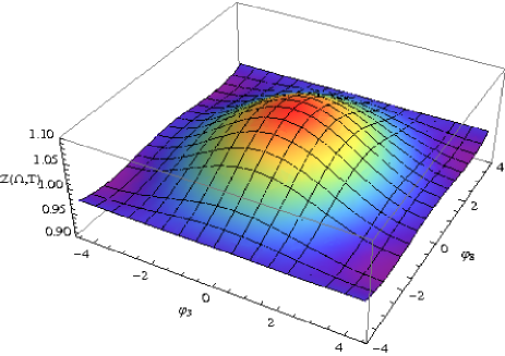
Figure 1: The function $Z(\Omega,T)$ on the plane $(\varphi_{3},\varphi_{8})$, for $T=70\,{\mathrm{MeV}}$. We have used $N_{f}=2$, considered as constituent quark and gluon masses $M_{q}=300\,{\mathrm{MeV}}$ and $M_{g}=664\,{\mathrm{MeV}}$ respectively, and the volume rule $V_{\sigma}=8\pi T^{3}/\sigma^{3}$ with $\sigma=(425\,{\mathrm{MeV}})^{2}$.

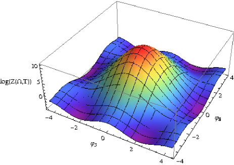
Figure 2: The function $\log Z(\Omega,T)$ on the plane $(\varphi_{3},\varphi_{8})$, for $N_{f}=2$ and $T=300\,{\mathrm{MeV}}$. See Fig. 1 for other details.

The behavior of $Z(\Omega,T)$ at high temperatures follows from Fig. 3 where the ratio $\log Z(\Omega,T)$ over $T^{6}$ is displayed. The existence of a limiting profile implies that all the functions $Z_{\mu}(T)$ grow exponentially as $\exp(\kappa T^{6})$. As discussed below for the bag model, a state-independent cavity of volume $V$ yields a behavior $\exp(\kappa VT^{3})$. The power $T^{6}$ is a consequence of the modeling $V_{\sigma}\sim T^{3}$ and mimics, in the constituent model, the Hagedorn behavior displayed by the MIT bag.

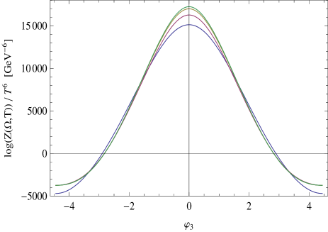
Figure 3: Plots of $(\log Z(\Omega,T))/T^{6}$ as a function of $\varphi_{3}$ for $\varphi_{8}=0$, for $N_{f}=2$ and several temperatures: from bottom to top $T=0.3,\,1,\,2$ and $5\,\,{\mathrm{GeV}}$.

In what follows we present analytic results for the Polyakov loop based on expansions in the number of constituents. These are obtained following the method already explained for Eq. (54). We consider the two types of estimates for $\langle\chi_{\mu}(\Omega)\rangle$ discussed at the end of Sec. II.1, namely,

$$\tilde{L}_{\mu}(T)=\frac{Z_{\mu}(T)}{Z_{\bf 1}(T)},\qquad L_{\mu}(T)=Z_{\mu,{\rm irred}}(T).$$ (69)

In the first expression the partition functions contain all types of color configurations (reducible and irreducible). In the second one only irreducible configurations are retained.

For the singlet partition function (i.e., the partition function in the absence of any colored source) one obtains

$$Z_{\bf 1} = 1+\frac{1}{2}\left(G_{1}^{2}+G_{2}+2Q_{1}\bar{Q}_{1}\right)$$ (70)

$$+\frac{1}{6}\left(2G_{1}^{3}+4G_{3}+6G_{1}Q_{1}\bar{Q}_{1}+Q_{1}^{3}+3Q_{1}Q_{2}+2Q_{3}+\bar{Q}_{1}^{3}+3\bar{Q}_{1}\bar{Q}_{2}+2\bar{Q}_{3}\right)$$

$$+\frac{1}{6}\big{(}2G_{1}^{4}+3G_{2}^{2}-2G_{3}G_{1}+3G_{4}+3(3G_{1}^{2}+G_{2})Q_{1}\bar{Q}_{1}+2G_{1}(Q_{1}^{3}-Q_{3}+\bar{Q}_{1}^{3}-\bar{Q}_{3})$$

$$+3Q_{1}^{2}\bar{Q}_{1}^{2}+3Q_{2}\bar{Q}_{2}\big{)}+O(c^{5}).$$

Here we have defined

$$Q_{n}(T) = 2N_{f}V_{\sigma}J(M_{q},T/n)+c\,e^{-nM_{q}/T}\,,$$ (71)

$$G_{n}(T) = 2V_{\sigma}J(M_{g},T/n)+c\,e^{-nM_{g}/T}\,,$$ (72)

for quarks and gluons respectively, and we choose $c=1$. The quantity $\bar{Q}_{n}$ is numerically identical to $Q_{n}$ but we distinguish both quantities in order to display the content of each term in the constituents: each factor $Q_{n}$, $\bar{Q}_{n}$ or $G_{n}$ count as $n$ quarks, antiquarks or gluons, respectively. So for instance, a term $G_{1}G_{2}Q_{3}\bar{Q}_{1}^{2}$ has a content $g^{3}q^{3}\bar{q}^{2}$.

If $Q_{n}$, $\bar{Q}_{n}$ and $G_{n}$ are replaced, respectively, by $\gamma_{q}q^{n}$, $\gamma_{\bar{q}}{\bar{q}}^{n}$, and $\gamma_{g}g^{n}$, in $Z_{\bf 1}$, the formulas for the singlet labeled as “Total” in Table 3 are reproduced. A similar statement holds for any irrep.

For the irreps of lowest order the expansions produce

$$\tilde{L}_{\bf 3} = \bar{Q}_{1}$$ (73)

$$+\frac{1}{2}\left(2G_{1}\bar{Q}_{1}+Q_{1}^{2}+Q_{2}\right)$$

$$+G_{1}\left(G_{1}\bar{Q}_{1}+Q_{1}^{2}\right)$$

$$+\frac{1}{24}\big{(}4(5G_{1}^{3}-3G_{1}G_{2}-2G_{3})\bar{Q}_{1}+6G_{1}^{2}\left(5Q_{1}^{2}-Q_{2}\right)-6G_{2}(Q_{1}^{2}-Q_{2})$$

$$-4(Q_{1}^{3}+3Q_{1}Q_{2}+2Q_{3})\bar{Q}_{1}-\bar{Q}_{1}^{4}-6\bar{Q}_{2}\bar{Q}_{1}^{2}-8\bar{Q}_{1}\bar{Q}_{3}-3\bar{Q}_{2}^{2}-6\bar{Q}_{4}\big{)}+O(c^{5}),$$

$$\tilde{L}_{\bf 6} = \frac{1}{2}\left(2G_{1}Q_{1}+\bar{Q}_{1}^{2}-\bar{Q}_{2}\right)$$ (74)

$$+\frac{1}{2}\left(2G_{1}\bar{Q}_{1}^{2}+(3G_{1}^{2}-G_{2})Q_{1}+\left(Q_{1}^{2}+Q_{2}\right)\bar{Q}_{1}\right)$$

$$+\frac{1}{12}\big{(}6(3G_{1}^{3}-G_{1}G_{2})Q_{1}+12G_{1}Q_{1}^{2}\bar{Q}_{1}+18G_{1}^{2}\bar{Q}_{1}^{2}-6G_{2}\bar{Q}_{2}+Q_{1}^{4}-4Q_{1}Q_{3}+3Q_{2}^{2}\big{)}+O(c^{5}),$$

$$\tilde{L}_{\bf 8} = G_{1}$$ (75)

$$+\left(G_{1}^{2}+Q_{1}\bar{Q}_{1}\right)$$

$$+\frac{1}{6}\left(5G_{1}^{3}-3G_{1}G_{2}-2G_{3}+12G_{1}Q_{1}\bar{Q}_{1}+2Q_{1}^{3}-2Q_{3}+2\bar{Q}_{1}^{3}-2\bar{Q}_{3}\right)$$

$$+\frac{1}{6}\big{(}3G_{1}^{2}(G_{1}^{2}-G_{2})+3(5G_{1}^{2}-G_{2})Q_{1}\bar{Q}_{1}$$

$$+G_{1}(5Q_{1}^{3}-3Q_{1}Q_{2}-2Q_{3}+5\bar{Q}_{1}^{3}-3\bar{Q}_{1}\bar{Q}_{2}-2\bar{Q}_{3})\big{)}+O(c^{5}),$$

$$\tilde{L}_{\bf 10} = \frac{1}{2}\left(G_{1}^{2}-G_{2}\right)$$ (76)

$$+\frac{1}{6}\left(4G_{1}^{3}+2G_{3}+6G_{1}Q_{1}\bar{Q}_{1}+\bar{Q}_{1}^{3}-3\bar{Q}_{1}\bar{Q}_{2}+2\bar{Q}_{3}\right)$$

$$+\frac{1}{12}\big{(}7G_{1}^{4}-3G_{2}^{2}-4G_{1}G_{3}+24G_{1}^{2}Q_{1}\bar{Q}_{1}+G_{1}\left(4Q_{1}^{3}-4Q_{3}+6\bar{Q}_{1}^{3}-6\bar{Q}_{1}\bar{Q}_{2}\right)$$

$$+3\left(Q_{1}^{2}+Q_{2}\right)\left(\bar{Q}_{1}^{2}-\bar{Q}_{2}\right)\big{)}+O(c^{5}),$$

$$\tilde{L}_{\bf 15^{\prime}} = \frac{1}{2}\left(G_{1}^{2}-G_{2}\right)\bar{Q}_{1}$$ (77)

$$+\frac{1}{24}\big{(}12G_{1}Q_{1}\left(\bar{Q}_{1}^{2}-\bar{Q}_{2}\right)+12G_{1}^{2}Q_{1}^{2}-12G_{2}Q_{2}+24G_{1}^{3}\bar{Q}_{1}$$

$$+\bar{Q}_{1}^{4}-6\bar{Q}_{1}^{2}\bar{Q}_{2}+8\bar{Q}_{1}\bar{Q}_{3}+3\bar{Q}_{2}^{2}-6\bar{Q}_{4}\big{)}+O(c^{5}),$$

$$\tilde{L}_{\bf 15} = G_{1}\bar{Q}_{1}$$ (78)

$$+\frac{1}{2}\left(4G_{1}^{2}\bar{Q}_{1}+2G_{1}Q_{1}^{2}+Q_{1}(\bar{Q}_{1}^{2}-\bar{Q}_{2})\right)$$

$$+\frac{1}{24}\big{(}12(5G_{1}^{3}-G_{1}G_{2})\bar{Q}_{1}+6G_{1}^{2}(9Q_{1}^{2}-Q_{2})-6G_{2}(Q_{1}^{2}-Q_{2})$$

$$+12G_{1}Q_{1}(3\bar{Q}_{1}^{2}-\bar{Q}_{2})+8(Q_{1}^{3}-Q_{3})\bar{Q}_{1}+3\bar{Q}_{1}^{4}-6\bar{Q}_{2}\bar{Q}_{1}^{2}-3\bar{Q}_{2}^{2}+6\bar{Q}_{4}\big{)}+O(c^{5}),$$

$$\tilde{L}_{\bf 24} = \frac{1}{2}G_{1}\left(2G_{1}\bar{Q}_{1}+Q_{1}^{2}-Q_{2}\right)$$ (79)

$$+\frac{1}{6}\big{(}6G_{1}Q_{1}\bar{Q}_{1}^{2}+12G_{1}^{3}\bar{Q}_{1}+3G_{1}^{2}\left(3Q_{1}^{2}-Q_{2}\right)$$

$$+\left(Q_{1}^{3}-3Q_{1}Q_{2}+2Q_{3}\right)\bar{Q}_{1}\big{)}+O(c^{5}),$$

$$\tilde{L}_{\bf 27} = \frac{1}{2}\left(G_{1}^{2}+G_{2}\right)$$ (80)

$$+\left(G_{1}Q_{1}\bar{Q}_{1}+G_{1}^{3}\right)$$

$$+\frac{1}{8}\big{(}9G_{1}^{4}+3G_{2}^{2}-2G_{4}-2G_{1}^{2}G_{2}+24G_{1}^{2}Q_{1}\bar{Q}_{1}$$

$$+4G_{1}\left(Q_{1}^{3}-Q_{1}Q_{2}+\bar{Q}_{1}^{3}-\bar{Q}_{1}\bar{Q}_{2}\right)+2\left(Q_{1}^{2}-Q_{2}\right)\left(\bar{Q}_{1}^{2}-\bar{Q}_{2}\right)\big{)}+O(c^{5}),$$

$$\tilde{L}_{\bf 35} = \frac{1}{3}\left(G_{1}^{3}-G_{3}\right)$$ (81)

$$+\frac{1}{8}(5G_{1}^{4}+2G_{1}^{2}G_{2}-G_{2}^{2}+2G_{4})+G_{1}^{2}Q_{1}\bar{Q}_{1}+\frac{1}{6}G_{1}\left(Q_{1}^{3}-3Q_{1}Q_{2}+2Q_{3}\right)+O(c^{5}),$$

$$\tilde{L}_{\bf 42} = \frac{1}{2}\left(G_{1}^{2}+G_{2}\right)\bar{Q}_{1}$$ (82)

$$+\frac{1}{4}\left(2G_{1}\left(G_{2}\bar{Q}_{1}+Q_{1}\left(\bar{Q}_{1}^{2}-\bar{Q}_{2}\right)\right)+6G_{1}^{3}\bar{Q}_{1}+G_{1}^{2}\left(3Q_{1}^{2}-Q_{2}\right)+G_{2}\left(Q_{1}^{2}+Q_{2}\right)\right)+O(c^{5}),$$

$$\tilde{L}_{\bf 64} = \frac{1}{6}\left(G_{1}^{3}+3G_{2}G_{1}+2G_{3}\right)+\frac{1}{2}\left(G_{1}^{2}+G_{2}\right)\left(G_{1}^{2}+Q_{1}\bar{Q}_{1}\right)+O(c^{5}).$$ (83)

For these same irreps, we have worked out the counting of irreducible color configurations for up to three constituents (see Table 1), and up to four constituents for the fundamental representation (see Table 2). As already noted, up to three constituents the two estimates coincide and the same property holds for any single-particle Hamiltonian, i.e.,

$$L_{\mu}(T)=\tilde{L}_{\mu}(T)+O(c^{4}).$$ (84)

The two estimates $L_{\mu}$ and $\tilde{L}_{\mu}$ differ by terms of $O(c^{5})$ for irreps beyond ${\bf 27}$, that require at least three constituents to be screened.

For the fundamental representation, up to four constituents, we find

$$L_{\bf 3} = \bar{Q}_{1}$$ (85)

$$+\frac{1}{2}\left(2G_{1}\bar{Q}_{1}+Q_{1}^{2}+Q_{2}\right)$$

$$+G_{1}\left(G_{1}\bar{Q}_{1}+Q_{1}^{2}\right)$$

$$+\frac{1}{4}(5G_{1}^{2}Q_{1}^{2}-G_{2}Q_{1}^{2}-G_{1}^{2}Q_{2}+G_{2}Q_{2})$$

$$+\frac{1}{6}(5G_{1}^{3}-3G_{1}G_{2}-2G_{3})\bar{Q}_{1}+O(c^{5}),$$

which differs from $\tilde{L}_{\bf 3}$ at $O(c^{4})$. $L_{\bf 3}$ reproduces the result quoted in Table 3.

We plot in Fig. 4 the Polyakov loop in the fundamental representation, computed within the two estimates, cf. Eqs. (73) and (85). The difference increases with temperature, but it is rather small $\lesssim 1\%$ already for temperatures close to the phase transition. In this figure it is shown also the difference between $Z_{\bf 3}$ and $L_{\bf 3}$, for which the values are noticeably larger. In Fig. 5 we display the Polyakov loop in several representations $\tilde{L}_{\mu}$. We have considered in these plots a phenomenological value for the constituent gluon mass, $M_{g}=664\,{\mathrm{MeV}}$, which leads to an exponential suppression at low temperature and it is consistent with strong coupling models of gluodynamics Meisinger et al. (2004).

We show in Figs. 6 and 7 the same information as in Fig. 5, but including only quarks and antiquarks in the first case, and only gluons in the latter. Only those irreps which lead to positive results are depicted. Exceptionally, the irreps ${\bf 10}$ and ${\bf 24}$ lead to negative results in the quarks and antiquarks contribution for $T<123\,{\mathrm{MeV}}$ and $T<171\,{\mathrm{MeV}}$ respectively, indicating that the prescription of Eq. (68) with $c=1$ is still insufficient in those cases. Note however that this does not happen in the gluonic terms, and the combined quark plus gluonic contribution is positive for all temperatures, c.f. Fig. 5.

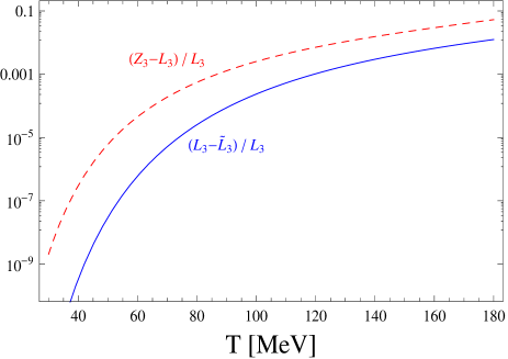
Figure 4: Difference between $Z_{{\rm PCM},{\bf 3}}$ and $L_{{\rm PCM},{\bf 3}}$ on the one hand, and between $L_{{\rm PCM},{\bf 3}}$ and $\tilde{L}_{{\rm PCM},{\bf 3}}$ on the other (normalized to $L_{{\rm PCM},{\bf 3}}$) as a function of $T$ (in $\,{\mathrm{MeV}}$), cf. Eqs. (73)-(85). In this plot we have included up to four constituents for the solid blue line, and up to three constituents for the dashed red line. See Fig. 1 for other details.

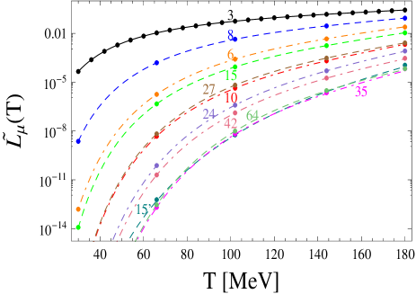
Figure 5: $\tilde{L}_{{\rm PCM},\mu}$ as a function of $T$ (in $\,{\mathrm{MeV}}$), for several irreps. From top to bottom $\mu={\bf 3}$, ${\bf 8}$, ${\bf 6}$, ${\bf 15}$, ${\bf 27}$, ${\bf 10}$, ${\bf 24}$, ${\bf 42}$, ${\bf 64}$, ${\bf 15^{\prime}}$, and ${\bf 35}$. Lines correspond to the result using the analytical formulas up to four constituents, cf. Eqs. (73)-(83), while points are the numerical result to all orders. We include only a few points for irreps other than ${\bf 3}$, for the clarity and appearance of the figure. See Fig. 1 for other details.

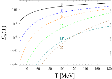
Figure 6: As Fig. 5 but including only quarks and antiquarks. Irreps ${\bf 35}$, ${\bf 42}$ and ${\bf 64}$ lead to values for the Polyakov loop identically zero. See text for discussion on other irreps.

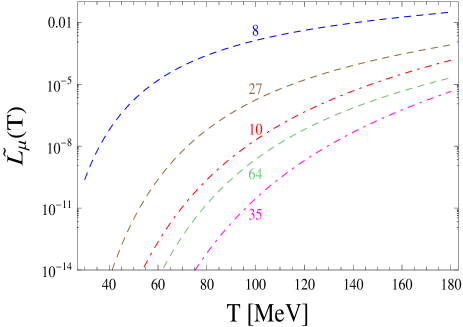
Figure 7: As Fig. 5 but including only gluons. Irreps ${\bf 3}$, ${\bf 6}$, ${\bf 15}$, ${\bf 15^{\prime}}$, ${\bf 24}$ and ${\bf 42}$ lead to values for the Polyakov loop identically zero.

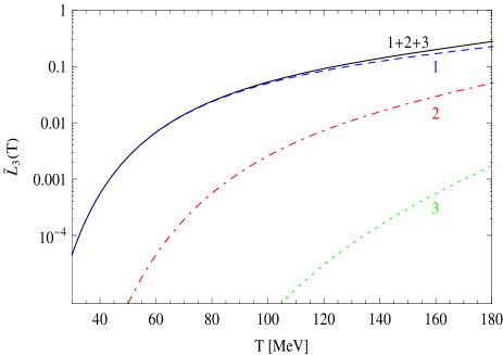
Figure 8: $\tilde{L}_{{\rm PCM},{\bf 3}}$ as a function of $T$ (in $\,{\mathrm{MeV}}$). Labels 1, 2 and 3 correspond to configurations with one, two and three constituents, respectively. $1+2+3$ corresponds to the sum of all the configurations up to three constituents.

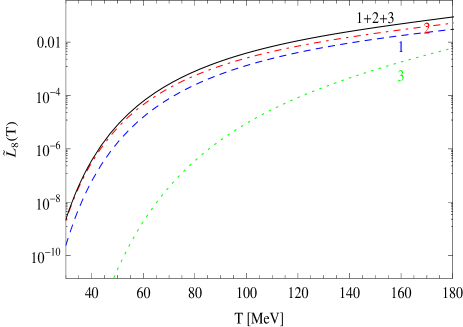
Figure 9: As in Fig. 8 for the adjoint representation.

It is shown in Figs. 8 and 9 the separate contribution of configurations with one, two and three constituents in $\tilde{L}_{\bf 3}$ and $\tilde{L}_{\bf 8}$. The convergence of the results is manifest. Fig. 10 displays the behavior of $\tilde{L}_{\bf 3}$ for a wider range of temperatures. The numerical result including all orders in the expansion in the number of constituents tend to the value $n_{\bf 3}=3$ at high temperatures. One can see in the figure that the analytical formulas, valid at low temperatures, break down at $T\approx 250\,{\mathrm{MeV}}$ when up to four constituents are included. In order to compare all the representations, we plot in Fig. 11 the result of $\tilde{L}_{\mu}/n_{\mu}$ including all orders in the expansion in the number of constituents. The value of the Polyakov loop in the representation $\mu$ tends to $n_{\mu}$ at high temperature. Note however that higher representations suffer a stronger “Polyakov cooling” Megias et al. (2006a). A consequence of that is that the inflexion temperature is shifted towards higher values for representations with increasing dimensionality. The upward shift of the curves has to do with the higher masses of the relevant states in higher representations.

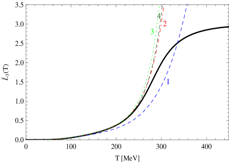
Figure 10: $\tilde{L}_{{\rm PCM},{\bf 3}}$ as a function of $T$ (in $\,{\mathrm{MeV}}$). Dashed lines represent the result using the analytical expansion up to one, two, three and four constituents, as indicated in the labels. The solid line correspond to the numerical result to all orders. See fig. 1 for other details.

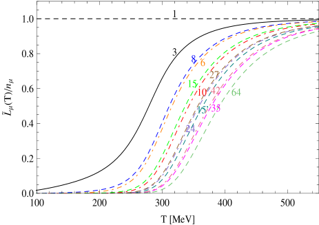
Figure 11: $\tilde{L}_{{\rm PCM},\mu}$ (normalized to $n_{\mu}$) as a function of $T$ (in $\,{\mathrm{MeV}}$), for several irreps. From top to bottom, $\mu={\bf 1}$, ${\bf 3}$, ${\bf 8}$, ${\bf 6}$, ${\bf 15}$, ${\bf 10}$, ${\bf 27}$, ${\bf 24}$, ${\bf 15^{\prime}}$, ${\bf 42}$, ${\bf 35}$, and ${\bf 64}$. The curves are obtained from the numerical result to all orders in the expansion in the number of constituents. See fig. 1 for other details.

V Estimates based on the bag model: selected configurations

In order to obtain an overall estimate of the spectrum of the heavy hadrons in the sum rule Eq. (7) we will use a simplified version of the MIT bag model Chodos et al. (1974); Hasenfratz and Kuti (1978). We expect that this approach will provide a picture of the Polyakov loop in different representations, and in particular, of the scaling rules at low temperatures. This would be an alternative to the Casimir scaling assumption, which is justified for temperatures above the crossover to the deconfining regime, where perturbation theory eventually applies.

Specifically, to obtain the spectrum of $\Delta$ (Eq. (7)), we consider states with zero, one or more quarks, antiquarks and gluons, occupying the allowed modes in the spherical cavity, and

$$\Delta = \min_{R}\left(\frac{1}{R}(\sum_{\alpha}n_{\alpha}\omega_{\alpha}-Z_{0})+\frac{4\pi}{3}R^{3}B\right)+\sum_{\alpha}n_{\alpha}m_{\alpha}$$ (86)

$$= T_{B}(\sum_{\alpha}n_{\alpha}\omega_{\alpha}-Z_{0})^{3/4}+\sum_{\alpha}n_{\alpha}m_{\alpha}\,.$$

Here $R$ is the bag radius, $Z_{0}$ a dimensionless parameter for the zero point energy, $B$ is the bag constant representing the QCD vacuum energy density, $\omega$ the modes in the spherical cavity and $m$ a mass term for the constituents (quarks, antiquarks, gluons) which we introduce additively. $n_{\alpha}$ is the occupation number of the spin-flavor state $\alpha$.

In the MIT bag, the radius is not fixed but selected in each hadron state by equating internal and external pressures. This produces the energy scale

$$T_{B}=\frac{4}{3}(4\pi B)^{1/4}.$$ (87)

Note that no center-of-mass corrections are required in $\Delta$, due to the infinite mass of the source.

In practice we take $Z_{0}=0$, and adopt $B=(166\,{\mathrm{MeV}})^{4}$. This corresponds to $T_{B}=416.7\,{\mathrm{MeV}}$. We include quarks with flavors $u$, $d$ and $s$, and take $m=0$ for $u$ and $d$ quarks, and also for gluons. For $s$ quarks we take $109\,{\mathrm{MeV}}$, although the limiting cases $m_{s}=0$ (three chiral flavors) and $m_{s}=\infty$ (two flavors), are also occasionally considered. In those limiting cases $B$, or equivalently $T_{B}$, is the only scale, so the calculation can be used directly for other values of $B$.

The modes in the spherical cavity are classified by the radial quantum number $n=1,2,\ldots$, the angular momentum $j=1/2,3/2,\ldots$ for quarks and antiquarks and $j=1,2,\ldots$ for gluons, the third component of angular momentum $m_{j}$, and the parity label $t=\pm 1$. This is taken such that the parity is $t(-1)^{j-1/2}$ for quarks, $t(-1)^{j+1/2}$ for antiquarks, and $t(-1)^{j}$ for gluons. The allowed values of $\omega$ are determined by the relations Bhaduri (1988); Barnes (1979):

$$0 = j_{j+1/2}(\omega)-j_{j-1/2}(\omega)\quad~{}~{}~{}(t=+1,\quad q~{}~{}\mbox{or}~{}~{}\bar{q}),$$

$$0 = j_{j+1/2}(\omega)+j_{j-1/2}(\omega)\quad~{}~{}~{}(t=-1,\quad q~{}~{}\mbox{or}~{}~{}\bar{q}),$$

$$0 = j_{j}(\omega)\qquad\qquad\qquad\qquad~{}~{}(t=+1,\quad\mbox{gluon}),$$

$$0 = \frac{j}{j+1}j_{j+1}(\omega)-j_{j-1}(\omega)\quad(t=-1,\quad\mbox{gluon}).$$ (88)

($\omega>0$, and $j_{\ell}$ is the $\ell$-th spherical Bessel function.) For a given type of particle, the $\omega$’s depend on the quantum numbers $(n,j,t)$. The lowest values of $\omega$ (i.e., $n=1$ and $j=1/2$ or $j=1$) for the four types of states in Eq. (88) are $2.043$, $3.812$, $4.493$, and $2.744$, respectively.

A MIT bag multiquark investigation, including the stability properties, was carried out in Ref. Zouzou and Richard (1994). The non-additivity of the quark model provides a further attraction for increasing number of quarks.

In general each bag state in the sum Eq. (7) is a multiparticle state composed of quarks, antiquarks and gluons, $q^{n_{q}}{\bar{q}}^{n_{\bar{q}}}g^{n_{g}}$, occupying certain bag levels, with color state coupled to the irrep $\bar{\mu}$. Note that, although the MIT bag is not strictly an independent particle system, the construction of Secs. III.2, III.3, and III.4 apply equally well in this case.

Numerical results for this section (MIT bag model and few constituents) are displayed in Appendix C together with the lowest bag states.

VI Estimates based on the bag model: all configurations

In this section we address the bag model calculation trying to include all possible sets of constituents. The goal is to sum up all possible fillings of irreducible type of the bag levels with constituents coupled to a given color irrep $\bar{\mu}$. Although in principle this is an improvement over the previous section, two problems appear: in this approach it is not practical to obtain separately the contributions of different sets of constituents, and more importantly, it is not obvious how to isolate the irreducible color configurations, i.e., the confining ones. So in this approach we have to content ourselves by obtaining some estimates.

In addition, in the MIT bag, the number of multiparticle states increases so quickly with the energy that the partition function diverges beyond a certain Hagedorn temperature Hagedorn (1965), as discussed e.g. in Kapusta (1981). The Hagedorn temperature, $T_{H}$, is lowered (and so more restrictive) as the number of species in the bag increases. We discuss this effect below.

VI.1 The fixed-radius bag system

If $H$ were the Hamiltonian of non-interacting particles, it would be immediate to express $Z$ in terms of sums over single particle states. The MIT bag introduces an attractive interaction through the rearrangement of the bag radius $R$, but its Hamiltonian has a particularly simple form which can be exploited by transforming it into an independent particle model looking form. To do so, we introduce an auxiliary bag system with a cavity of fixed radius $R$. The numerical value of $R$ is not relevant since this quantity is eliminated in the final result for the MIT bag. In addition, we introduce the following two non-interacting Hamiltonians (which obviously commute with each other)

$$H^{\prime}_{k}=\frac{1}{R}\sum_{\alpha,c}\omega_{\alpha}a_{\alpha,c}^{\dagger}a_{\alpha,c},\qquad H_{m}=\sum_{\alpha,c}m_{\alpha}a_{\alpha,c}^{\dagger}a_{\alpha,c}.$$ (89)

Here $\alpha$ and $c$ indicate the spin-flavor and color labels and $a_{\alpha,c}$ is the corresponding annihilation operator. To distinguish them from the MIT bag quantities, in what follows we use a prime to indicate quantities related to this auxiliary fixed-radius bag system.

In terms of these auxiliary one-body Hamiltonians, the Hamiltonian of the MIT bag model (i.e., with relaxation of $R$ to its most stable value) that reproduces Eq. (86), takes the form

$$H=T_{B}(RH^{\prime}_{k}-Z_{0})^{3/4}+H_{m}.$$ (90)

To proceed further let $f_{\frac{3}{4}}(t)$ denote the inverse Laplace transform of $e^{-s^{3/4}}$ (see Appendix B for details). This allows us to write the relation

$$Z(\Omega,T)=\int_{0}^{\infty}d\beta^{\prime}\bar{f}(\beta^{\prime},\beta)Z^{\prime}(\Omega,T^{\prime},T)\,,$$ (91)

where $T^{\prime}=1/\beta^{\prime}$,

$$\bar{f}(\beta^{\prime},\beta)=\frac{e^{\beta^{\prime}Z_{0}/R}}{R(\beta T_{B})^{4/3}}f_{\frac{3}{4}}\left(\frac{\beta^{\prime}}{R(\beta T_{B})^{4/3}}\right)\,,$$ (92)

and

$$Z^{\prime}(\Omega,T^{\prime},T)={\rm Tr}(e^{-\beta^{\prime}H^{\prime}_{k}-\beta H_{m}}\,U(\Omega)).$$ (93)

$Z^{\prime}(\Omega,T^{\prime},T)$ describes the partition function of a non-interacting system (with two temperatures), namely, that of a bag of fixed radius $R$. This systems does not have a Hagedorn temperature. Of course, this partition function can also be analyzed in terms of ${\mathrm{SU}}(3)$ irreps (similar to Eq. (33)) to give $Z^{\prime}_{\mu}(T^{\prime},T)$, and it follows that

$$Z_{\mu}(T)=\int_{0}^{\infty}d\beta^{\prime}\bar{f}(\beta^{\prime},\beta)Z^{\prime}_{\mu}(T^{\prime},T).$$ (94)

The virtue of $H^{\prime}_{k}$ and $H_{m}$ is that they are one-body operators, leading to a non-interacting system (more precisely, interacting just with an external potential) and this is not spoiled by the presence of $U(\Omega)$ (which is just equivalent to minimal coupling). Thus, using the expressions in terms of $T$ and $T^{\prime}$ we may profit from the results of section III.5 in a rather straightforward manner. In particular, the partition function of the fixed-radius system fulfills the factorization property as in Eq. (37),

$$Z^{\prime}=Z^{\prime}_{q}Z^{\prime}_{\bar{q}}Z^{\prime}_{g}\,,$$ (95)

where these partition functions are given now (compare with Eq. (38)) by

$$\log Z^{\prime}_{q}(\Omega,T^{\prime},T) = \sum_{\alpha}\!{}^{q}\,\gamma_{\alpha}\,\chi_{\bf 3}\!\left(\log(1+\Omega\,e^{-\beta^{\prime}\omega_{\alpha}/R-\beta m_{\alpha}})\right),$$

$$\log Z^{\prime}_{\bar{q}}(\Omega,T^{\prime},T) = \sum_{\alpha}\!{}^{\bar{q}}\,\gamma_{\alpha}\,\chi_{\bf\bar{3}}\!\left(\log(1+\Omega\,e^{-\beta^{\prime}\omega_{\alpha}/R-\beta m_{\alpha}})\right),$$

$$\log Z^{\prime}_{g}(\Omega,T^{\prime},T) = -\sum_{\alpha}\!{}^{g}\,\gamma_{\alpha}\,\chi_{\bf 8}\!\left(\log(1-\Omega\,e^{-\beta^{\prime}\omega_{\alpha}/R-\beta m_{\alpha}})\right)\,.$$

Likewise, the following symmetry properties hold

$$Z^{\prime}_{\bar{q}}=(Z^{\prime}_{q})^{*},\qquad Z^{\prime}_{g}=(Z^{\prime}_{g})^{*}.$$ (97)

Similarly, we can introduce the auxiliary $\Omega$-independent functions

$$z^{\prime}_{q}(T^{\prime},T) = \sum_{\alpha}\!{}^{q}\,\gamma_{\alpha}\,e^{-\beta^{\prime}\omega_{\alpha}/R-\beta m_{\alpha}},$$

$$z^{\prime}_{g}(T^{\prime},T) = \sum_{\alpha}\!{}^{g}\,\gamma_{\alpha}\,e^{-\beta^{\prime}\omega_{\alpha}/R-\beta m_{\alpha}},$$ (98)

and the relation corresponding to Eq. (41) becomes

$$\log Z^{\prime}_{q}(\Omega,T^{\prime},T) = \sum_{n=1}^{\infty}\frac{(-1)^{n+1}}{n}\,\chi_{\bf 3}(\Omega^{n})\,z^{\prime}_{q}(T^{\prime}/n,T/n),$$

$$\log Z^{\prime}_{g}(\Omega,T^{\prime},T) = \sum_{n=1}^{\infty}\frac{1}{n}\,\chi_{\bf 8}(\Omega^{n})\,z^{\prime}_{g}(T^{\prime}/n,T/n).$$ (99)

The antifundamental and adjoint characters can be reduced to the fundamental one using Eq. (42). The analogous of Eq. (44) is then

$$\log\hat{Z}^{\prime}_{q}(\omega,T^{\prime},T) = \sum_{n=1}^{\infty}\frac{(-1)^{n+1}}{n}\,\omega^{n}\,z^{\prime}_{q}(T^{\prime}/n,T/n),$$

$$\log\hat{Z}^{\prime}_{g}(\omega,T^{\prime},T) = \sum_{n=1}^{\infty}\frac{1}{n}\,\omega^{n}\,z^{\prime}_{g}(T^{\prime}/n,T/n).$$ (100)

Finally,

$$\log Z^{\prime}_{q}(\Omega,T^{\prime},T) = \sum_{i=1}^{3}\log\hat{Z}^{\prime}_{q}(\omega_{i},T^{\prime},T),$$

$$\log Z^{\prime}_{g}(\Omega,T^{\prime},T) = \sum_{i,j=1}^{3}\log\hat{Z}^{\prime}_{g}(\omega_{i}\omega_{j}^{*},T^{\prime},T)-\log\hat{Z}^{\prime}_{g}(1,T^{\prime},T)\,.$$

Before going any further, let us give more details on the functions $z^{\prime}_{q}$ and $z^{\prime}_{g}$. If we assume $N_{f}$ massless flavors, and $N_{f}^{\prime}$ degenerated flavors with mass $m_{s}$, as well as massless gluons, we can write

$$z^{\prime}_{q}(T^{\prime},T) = (N_{f}+N^{\prime}_{f}e^{-\beta m_{s}})\sum_{\alpha}\!{}^{q}\,\gamma_{\alpha}\,e^{-\beta^{\prime}\omega_{\alpha}/R},$$

$$z^{\prime}_{g}(T^{\prime},T) = \sum_{\alpha}\!{}^{g}\,\gamma_{\alpha}\,e^{-\beta^{\prime}\omega_{\alpha}/R}.$$ (102)

Here $\sum_{\alpha}^{q}$ no longer includes flavor. For both, quarks and gluons, $\alpha=(n,j,t)$ and $\gamma_{\alpha}=2j+1$. So numerically, we need to compute functions of a single variable $T^{\prime}$.

The sums over levels are not finite. To deal with this problem, say for gluons, we separate the level sums as

$$z_{g}^{\prime}(T^{\prime})=(\sum_{\omega_{\alpha}<\omega_{\rm max}}+\sum_{\omega_{\alpha}\geq\omega_{\rm max}})\,\gamma_{\alpha}\,e^{-\beta^{\prime}\omega_{\alpha}/R}:=z^{\prime}_{<}(T^{\prime})+z^{\prime}_{>}(T^{\prime}).$$ (103)

The finite sum $z^{\prime}_{<}(T^{\prime})$ is done numerically. On the other hand, $z^{\prime}_{>}(T^{\prime})$ is approximated using the asymptotic form of the spectrum. As is very well-known from the black-body problem, the cumulative number of single-particle states in a cavity of volume $V$ is $N_{1}(E)=VE^{3}/(3\pi^{2})$ plus terms that are subdominant for large $E$. We have included a spin degeneracy factor of $2$ valid for both quarks and gluons. For our spherical bag of radius $R$, this gives for the cumulative number of states and the corresponding density of single-particle levels in the large $E$ region

$$N_{1}(E)\approx\frac{4}{9\pi}R^{3}E^{3},\quad\rho_{1}(E)\approx\frac{4}{3\pi}R^{3}E^{2}.$$ (104)

This allows us to write

$$z^{\prime}_{>}(T^{\prime}) = \int_{\omega_{\rm max}/R}^{+\infty}dE\rho_{1}(E)\,e^{-\beta^{\prime}E}$$

$$\approx \frac{4}{3\pi}R^{3}T^{\prime}\left[\left(\frac{\omega_{\rm max}}{R}+T^{\prime}\right)^{2}+T^{\prime}{}^{2}\right]e^{-\beta^{\prime}\omega_{\rm max}/R}.$$

This asymptotic expression of $z^{\prime}_{>}(T^{\prime})$ holds both for quarks and gluons. In our calculation we have taken $\omega_{\rm max}=100$, although a much smaller value would probably be sufficient. We have verified that $z^{\prime}_{q,g}(T^{\prime},T)$ are not sensitive to this particular choice of $\omega_{\rm max}$.

Although certainly possible, it is technically more difficult to deal with functions of several variables, so in what follows we consider just $N_{f}$ massless quark flavors and $N^{\prime}_{f}=0$ in Eq. (102). The choices $N_{f}=2$ ($N_{f}=3$) would correspond to taking the limit of a heavy (light) strange quark. $N_{f}=0$ corresponds to gluodynamics. As a consequence, the dependence on $T$ disappears in the various primed functions. In addition, $R$ or $T_{B}$ become the only scale, for fixed-radius bag and MIT bag systems, respectively.

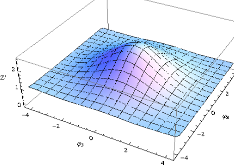
Figure 12: The function $Z^{\prime}(\Omega,T^{\prime})$ on the plane $(\varphi_{3},\varphi_{8})$, for $N_{f}=3$ and $RT^{\prime}=1/2$.

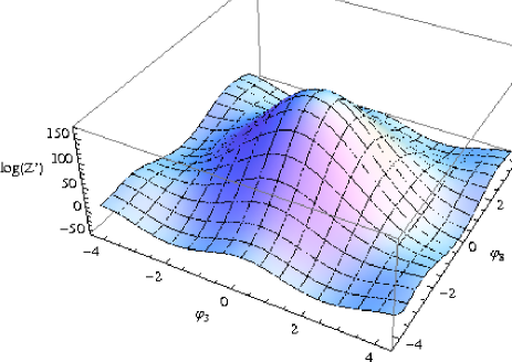
Figure 13: The function $\log Z^{\prime}(\Omega,T^{\prime})$ on the plane $(\varphi_{3},\varphi_{8})$, for $N_{f}=3$ and $RT^{\prime}=2$.

In the fixed bag-radius problem the partition function converges for all temperatures $T^{\prime}$, nevertheless, this function increases rather quickly with the temperature. In Fig. 12 we display $Z^{\prime}(\Omega,T^{\prime})$ as a function of $\Omega$ (in the plane $(\varphi_{3},\varphi_{8})$) for $N_{f}=3$ and $RT^{\prime}=0.5$. As shown in Eq. (33), the central value $Z^{\prime}(\Omega=1,T^{\prime})$ is just the full partition function, adding all irreps. In Fig. 13 we display the logarithm of the same function, this time for $RT^{\prime}=2$. The direct plot of the partition function would look similar to a two-dimensional Dirac delta distribution centered at $\Omega=1$ in the plane $(\varphi_{3},\varphi_{8})$, with a certain normalization. This suggests that in the large-$T^{\prime}$ limit, we would have

$$\frac{Z^{\prime}(\Omega,T^{\prime})}{\int d\Omega^{\prime}Z^{\prime}(\Omega^{\prime},T^{\prime})} = \frac{1}{Z^{\prime}_{\bf 1}(T^{\prime})}\sum_{\mu}\chi^{*}_{\mu}(\Omega)Z^{\prime}_{\mu}(T^{\prime})$$ (106)

$$\underset{T^{\prime}\to\infty}{\sim} \delta(\Omega,1)=\sum_{\mu}n_{\mu}\chi^{*}_{\mu}(\Omega).$$

Therefore, in the large temperature limit

$$\frac{Z^{\prime}_{\mu}(T^{\prime})}{Z^{\prime}_{\bf 1}(T^{\prime})}\sim n_{\mu}.$$ (107)

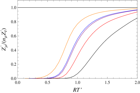
Figure 14: Plot of $Z^{\prime}_{\mu}(T^{\prime})/(n_{\mu}Z^{\prime}_{\bf 1}(T^{\prime}))$ as a function of $RT^{\prime}$ for several irreps. From top to bottom, $\mu={\bf 1}$, ${\bf 3}$, ${\bf 8}$, ${\bf 6}$, ${\bf 10}$, and ${\bf 64}$. Note that the ratio $Z^{\prime}_{\mu}/Z^{\prime}_{\bf 1}$ is just the estimate $\tilde{L}^{\prime}_{\mu}$ introduced below, in Eq. (119).

This conjecture is indeed supported by the numerical results shown in Fig. 14. The interpretation is that of an equipartition of populations between all available modes, in the large temperature limit.

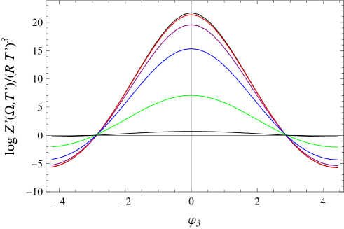
Figure 15: Plots of $(\log Z^{\prime}(\Omega,T^{\prime}))/(RT^{\prime})^{3}$ as a function of $\varphi_{3}$ for $\varphi_{8}=0$, for $N_{f}=3$ and several temperatures: from bottom to top $RT^{\prime}=0.25,0.5,1,2,5,10$. The theoretical large-$T^{\prime}$ limit at the maximum is $19(\pi/3)^{3}=21.82$. Remarkably the value of $\varphi_{3}$ for which $Z^{\prime}(\Omega,T^{\prime})=1$ turns out to be very similar (although not exactly equal) for all temperatures, namely, $\varphi_{3}=2.9$. For gluons and for quarks a similar effect takes place at $\varphi_{3}=2.2$ and $2.99$, respectively.

The function $Z^{\prime}(\Omega,T^{\prime})$ increases very rapidly with the temperature and this directly causes the existence of a Hagedorn temperature for $Z(\Omega,T)$. In order to investigate whether the same critical temperature exists for the functions $Z_{\mu}(T)$ we need to see the large temperature behavior of the $Z^{\prime}_{\mu}(T^{\prime})$. To this end, we display in Fig. 15 the ratio $\log Z^{\prime}(\Omega,T^{\prime})$ over $(RT^{\prime})^{3}$, on the $\varphi_{3}$ axis (the plot on the $\varphi_{8}$ axis is qualitatively similar), for several temperatures. The plot suggests that the ratio tends to a fixed limiting profile $P(\Omega)$

$$P(\Omega)=\lim_{T^{\prime}\to\infty}\frac{\log Z^{\prime}(\Omega,T^{\prime})}{(RT^{\prime})^{3}}.$$ (108)

This function has its absolute maximum at $\Omega=1$. (Obvious modifications apply when $N_{f}=0$, due to center symmetry.) The existence and shape of the limiting function $P(\Omega)$ implies that the height of $Z^{\prime}(\Omega,T^{\prime})$ increases exponentially as $\exp(\kappa(RT^{\prime})^{3})$ (with $\kappa=P(1)$) while its width in the $\Omega$ plane decreases as a power, $1/(RT^{\prime})^{3/2}$. Therefore the integral $Z^{\prime}_{\bf 1}(T^{\prime})$, as well as all other $Z^{\prime}_{\mu}(T^{\prime})$, grow exponentially at a common rate $\exp(\kappa(RT^{\prime})^{3})$. As a consequence the Hagedorn temperature is common to all irreps. The argument also shows that the total number of active irreps at a temperature $T^{\prime}$ grows at a rate $(RT^{\prime})^{3}$.

VI.2 Hagedorn temperature

The existence of a critical temperature, $T_{H}$, in the MIT bag was noted very early Chodos et al. (1974). In order to determine the value of $T_{H}$, we first obtain the asymptotic form of $Z^{\prime}(T^{\prime})$ at large temperatures. This can be done by using the asymptotic form of the single-particle level density $\rho_{1}(E)$ in Eq. (104). This yields $z^{\prime}_{g}(T^{\prime})\sim(8/3\pi)(RT^{\prime})^{3}$ for gluons, with an extra factor $N_{f}$ for quarks. These expressions can be inserted in Eq. (100) (here it enters the Riemann $\zeta$ function) and then in Eq. (LABEL:eq:4.20) for $\Omega=1$. Adding the contributions from quarks, antiquarks and gluons, this finally produces

$$\log Z^{\prime}(T^{\prime})\sim\kappa\,R^{3}T^{\prime}{}^{3},$$

$$\kappa=\frac{\pi^{3}}{135}(7N_{c}N_{f}+4(N_{c}^{2}-1)),$$ (109)

where $N_{c}=3$ is the number of colors. For $N_{f}=3$, this value of $\kappa$ reproduces the large-$T^{\prime}$ limit at the maximum in Fig. 15. Of course, the asymptotic form in Eq. (109) is nothing else than the well-known result for the partition function of a gas of free massless particles in a volume $V=(4\pi/3)R^{3}$, and we have just checked the consistency of our formulas.

The parameter $\kappa$ controls the Hagedorn temperature. Let $\rho^{\prime}(E^{\prime})$ denote the multiparticle density of energy levels in the fixed-radius bag system,

$$Z^{\prime}(T^{\prime})=\int_{0}^{\infty}dE^{\prime}\,\rho^{\prime}(E^{\prime})\,e^{-\beta^{\prime}E^{\prime}}.$$ (110)

The behavior in the asymptotic regime of large energies and temperatures can be obtained by using a saddle point approximation in the integral together with Eq. (109). This gives, for the cumulative number of states,

$$N^{\prime}(E^{\prime})\sim e^{\frac{4}{3}(3\kappa)^{1/4}(RE^{\prime})^{3/4}}.$$ (111)

The MIT bag and fixed-radius bag Hamiltonians are functionally related, namely, $H=T_{B}(RH^{\prime}_{k})^{3/4}$. The same functional relation follows for the eigenvalues, $E=T_{B}(RE^{\prime})^{3/4}$, while degeneracies are unchanged. It follows that the cumulative number of states transforms as a scalar quantity, $N(E)=N^{\prime}(E^{\prime})$. This immediately implies

$$N(E)\sim e^{E/T_{H}},\qquad T_{H}=\frac{3}{4}\frac{T_{B}}{(3\kappa)^{1/4}}=\left(\frac{4\pi B}{3\kappa}\right)^{1/4}.$$ (112)

This coincides with standard result Kapusta (1981). Here we see that the effective attraction between constituents, leading to rearrangement of the radius of the bag, produces a slide in the multi-particle spectrum. Higher states are brought down in such a way that $N^{\prime}(E^{\prime})$ goes into $N(E)$.

Similar relations hold when $\Omega$ is present. As for the partition function, one can introduce the cumulative number of states and density of levels,

$$N(\Omega,E) = {\rm Tr}(\Theta(E-H)U(\Omega)),$$

$$\rho(\Omega,E) = {\rm Tr}(\delta(E-H)U(\Omega)),$$ (113)

and analogously for the primed system. Likewise, the scalar transformation property still holds in the presence of $\Omega$,

$$N(\Omega,E)=N^{\prime}(\Omega,E^{\prime}).$$ (114)

As discussed previously, the $Z^{\prime}_{\mu}(T^{\prime})$ all grow exponentially with a common rate $e^{\kappa(RT^{\prime})^{3}}$, and this implies a common limiting temperature equal to $T_{H}$ for all the $Z_{\mu}(T)$. The situation for $Z(\Omega,T)$ is slightly different. $Z^{\prime}(\Omega,T^{\prime})$ grows at an $\Omega$-dependent rate $e^{P(\Omega)(RT^{\prime})^{3}}$, so in this case we expect also an $\Omega$-dependent critical temperature

$$T_{c}(\Omega)=(\kappa/P(\Omega))^{1/4}T_{H}\geq T_{H}.$$ (115)

This critical temperature coincides with $T_{H}$ when $\Omega$ is the identity element and increases as $\Omega$ departs from it.

In order to obtain the partition function $Z(\Omega,T)$ itself, we have to apply Eq. (91). The small-$t$ asymptotic form of $f_{\frac{3}{4}}(t)$, Eq. (145), implies the following large-$T^{\prime}$ behavior

$$\bar{f}(\beta^{\prime},\beta)\sim\frac{1}{R}\left(\frac{T}{T_{B}}\right)^{4/3}e^{-\frac{1}{3}(RT^{\prime})^{3}\left(\frac{3}{4}\frac{T_{B}}{T}\right)^{4}}.$$ (116)

From the asymptotic form of $Z^{\prime}(\Omega,T^{\prime})$ it follows that the $\beta^{\prime}$ integral in Eq. (91) diverges at small $\beta^{\prime}$ when $T\geq T_{c}(\Omega)$, as expected.

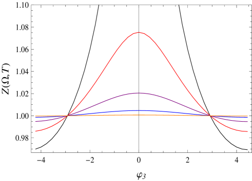
Figure 16: The function $Z(\Omega,T)$ on the $\varphi_{3}$ axis, for $N_{f}=3$ and for several temperatures. From bottom to top, $T/T_{B}=0.15625$, $0.1875$, $0.21875$, $0.25$, and $0.28125$. The last temperature is above $T_{H}$ and $Z$ diverges in a neighborhood of $\varphi_{3}=0$.

For $N_{f}=3$ (our preferred case) $T_{H}=0.2637\,T_{B}$, so we cannot consider temperatures larger that this in the calculation of $Z_{\mu}(T)$. The form of $Z(\Omega,T)$ at $T=0.25T_{B}$, for $N_{f}=3$ is displayed in Fig. 16.

Before ending this section, we briefly mention the large temperature behavior of the quark constituent model. The asymptotic forms discussed for the fixed-radius bag also apply for the quark constituent model by changing $V=(4\pi/3)R^{3}$ to $V=V_{\sigma}$. E.g. $N_{1}(E)\sim V_{\sigma}E^{3}/(3\pi^{2})$ at large energies (and this is consistent with the form of $J(0,T)$ in Eq. (67)). Consequently, at large temperatures

$$\log Z_{\rm PCM}(1,T)\sim\frac{3}{4\pi}\kappa V_{\sigma}T^{3},$$ (117)

where $\kappa$ is that of Eq. (109). The full dependence on the temperature requires to specify how $V_{\sigma}$ depends on $T$. An increasing function would imply a steeper dependence of $Z_{\rm PCM}$ on $T$, as compared to the fixed-radius cavity, and so effectively to attraction between constituents.

In general it should be expected that the constituent model behaves as the fixed-radius bag with volume $V_{\sigma}$. This is specially so for $T$ larger than $R^{-1}$ and $M$, since then the discrete spectrum of the cavity can be approximated by a continuous semiclassical one and the mass (not present in the bag) can also be disregarded.

VI.3 Irreducible color configurations

All the previous considerations refer to the partition functions $Z_{\mu}(T)$. These functions include all types of configurations, reducible and irreducible, as defined in Sec. III.3. We can introduce the corresponding irreducible version $L_{\mu}(T)$, which only includes the irreducible color configurations. $L_{\mu}(T)$ is the bag estimate of the Polyakov loop in the irrep $\mu$, introduced in Eq. (8). Using similar constructions to those in Eq. (31) and Eq. (33), one can define $L(T)$ (adding up all ${\mathrm{SU}}(3)$ irreps) and $L(\Omega,T)$. (Note that those relations are all linear.) Furthermore, we can also consider the fixed-radius bag versions, $L^{\prime}_{\mu}(T^{\prime},T)$, $L^{\prime}(T^{\prime},T)$, and $L^{\prime}(\Omega,T^{\prime},T)$. They will fulfill the corresponding versions of Eqs. (91) and (94):

$$L(\Omega,T) = \int_{0}^{\infty}d\beta^{\prime}\bar{f}(\beta^{\prime},\beta)L^{\prime}(\Omega,T^{\prime},T),$$

$$L_{\mu}(T) = \int_{0}^{\infty}d\beta^{\prime}\bar{f}(\beta^{\prime},\beta)L^{\prime}_{\mu}(T^{\prime},T).$$ (118)

The isolation of the irreducible configurations to obtain $L_{\mu}(T)$ or $L^{\prime}_{\mu}(T^{\prime},T)$ can be done for each given finite set of constituents. Unfortunately, we have not devised a method to do so when all such sets are taken together, i.e., in the form of a generating functional producing just the irreducible color configurations. In view of that, we take $Z$ (including all color configurations, irreducible or not) and $\tilde{L}$ (the ratio $Z/Z_{\bf 1}$) as upper and lower estimates of $L$.

The estimate of irreducible terms by the ratio $Z/Z_{\bf 1}$ makes sense (and it is exact to three constituents) only in the non interacting case, and so in the fixed-radius bag problem. So we define

$$\tilde{L}^{\prime}_{\mu}(T^{\prime},T):=\frac{Z^{\prime}_{\mu}(T^{\prime},T)}{Z^{\prime}_{\bf 1}(T^{\prime},T)},$$ (119)

and use it as a lower bound or estimate on the true $L^{\prime}_{\mu}(T^{\prime},T)$:

$$\tilde{L}^{\prime}_{\mu}(T^{\prime},T)\underset{\sim}{<}L^{\prime}_{\mu}(T^{\prime},T)\underset{\sim}{<}Z^{\prime}_{\mu}(T^{\prime},T).$$ (120)

From $\tilde{L}^{\prime}_{\mu}(T^{\prime},T)$ we then obtain a lower estimate $\tilde{L}_{\mu}(T)$ in the MIT bag by applying Eq. (118).

It is noteworthy that the lower estimates become exact in the low temperature limit: in this limit only the states with fewest constituents have a chance to get populated.

We do not know how $L_{\mu}(T)$ behaves as the temperature increases. However, using Eq. (118), setting $Z_{0}=N_{f}^{\prime}=0$ in the bag parameters as before, it follows that

$$L_{\mu}(T)=\int_{0}^{\infty}d\beta^{\prime}xf_{\frac{3}{4}}(x\beta^{\prime})L^{\prime}_{\mu}(T^{\prime}),\qquad x=\left(\frac{T}{T_{B}}\right)^{4/3}.$$ (121)

As $T\to\infty$, $xf_{\frac{3}{4}}(x\beta^{\prime})$ becomes a normalized Dirac delta at $\beta^{\prime}=0$, and therefore

$$\lim_{T\to\infty}L_{\mu}(T)=\lim_{T^{\prime}\to\infty}L^{\prime}_{\mu}(T^{\prime}).$$ (122)

As discussed above, the upper estimate $Z^{\prime}_{\mu}(T^{\prime},T)$ increases exponentially with the temperature, as $e^{\kappa(RT^{\prime})^{3}}$, and produces a divergence in the upper estimate of $L_{\mu}(T)$ for temperatures beyond $T_{H}$.

On the other hand, from Eq. (107) and Fig. 14, the lower estimate $\tilde{L}^{\prime}_{\mu}(T^{\prime},T)$ tends to a constant value $n_{\mu}$. Therefore, Eq. (122) implies for the MIT bag

$$\lim_{T\to\infty}\tilde{L}_{\mu}(T)=n_{\mu}.$$ (123)

This result is remarkable because it indeed coincides with the exact QCD result: for temperatures above the crossover, in the perturbative regime, the Polyakov loop tends to the identity element and so $L_{{\rm QCD},\mu}\to n_{\mu}$ . Nevertheless, there is no sound reason to believe that $\tilde{L}_{\mu}(T)$ should be a valid estimate of $L_{{\rm QCD},\mu}(T)$ at all temperatures. Certainly the true $L_{\mu}(T)$ (irreducible configurations in the MIT bag) increases without bound with $T$: even the simplest configuration $Q\bar{q}$ (heavy meson in $L_{\bf 3}$) contains an ever increasing set of single particle states that are activated as $T$ grows. What is less clear is whether $L_{\mu}(T)$ has a Hagedorn temperature, as $Z_{\mu}(T)$, since to settle that point requires to estimate the growth of the number of irreducible color configurations as compared to the total ones. As already noted, estimates based on the hadron resonance model are not reliable at temperatures above the QCD crossover.

Finally, in Figs. 17 and 18 we display the behavior of $\tilde{L}_{\mu}(T)$ for several irreps below the QCD crossover.

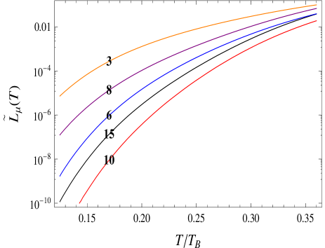
Figure 17: $\tilde{L}_{\mu}(T)$ as a function of $T/T_{B}$, for several irreps. From top to bottom $\mu={\bf 3}$, ${\bf 8}$, ${\bf 6}$, ${\bf 15}$, ${\bf 10}$.

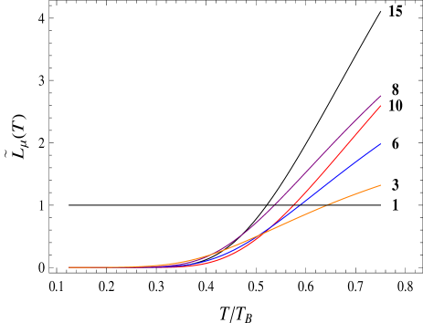
Figure 18: As Fig. 17 (in non logarithmic scale) for a wider range of temperatures. From bottom to top $\mu={\bf 1}$, ${\bf 3}$, ${\bf 6}$, ${\bf 10}$, ${\bf 8}$, ${\bf 15}$. The asymptotic value is $n_{\mu}$.

VII Polyakov loop scaling in single-particle models at low temperatures

At temperatures well below the crossover, the Boltzmann weight factor becomes determinant in selecting the dominant mechanisms contributing to the expectation value of the Polyakov loop in each irrep. In principle, this is very different from a Casimir scaling behavior, based on perturbative estimates, although in both cases higher irreps tend to be suppressed.

Sources carrying higher representations require a larger number of constituents for its screening, and this number gives the leading term in the low temperature scaling. From Table 1, in gluodynamics this counting gives (up to proportionality constants)

$$L_{\bf 10}\sim L_{\bf 27}\sim L_{\bf 8}^{2},\qquad L_{\bf 35}\sim L_{\bf 64}\sim L_{\bf 8}^{3}.$$ (124)

On the other hand, in QCD and assuming gluonic modes to be heavy, one obtains

$$L_{\bf 6}\sim L_{\bf 8}\sim L_{\bf 3}^{2},\qquad L_{\bf 10}\sim L_{\bf 15}\sim L_{\bf 3}^{3},\qquad L_{\bf 15^{\prime}}\sim L_{\bf 24}\sim L_{\bf 3}^{4}.$$ (125)

The previous scalings assume that a purely single-particle description is appropriate. In the MIT bag the energy is not strictly additive and deviations take place. Specifically, in gluodynamics the lightest mode is $1^{+}$ with $\omega_{g}=2.744$. Due to the symmetry of the gluon wavefunction, the degeneracies of $\mu={\bf 8}$, ${\bf 10}$, ${\bf 27}$, ${\bf 35}$, and ${\bf 64}$ are, respectively, $3$, $3$, $6$, $8$, and $10$ for the corresponding lightest states. Therefore, at low temperatures the model produces the following relations:

$$\log(\frac{1}{3}L_{\bf 8})\sim 2^{-3/4}\log(\frac{1}{3}L_{\bf 10})\sim 3^{-3/4}\log(\frac{1}{8}L_{\bf 35}),$$

$$L_{\bf 27}\sim 2L_{\bf 10},\qquad L_{\bf 64}\sim\frac{4}{5}L_{\bf 35}.$$ (126)

In QCD, the lightest quark mode is $\frac{1}{2}^{+}$, with $\omega_{q}=2.043$. For $\mu={\bf 3}$ and ${\bf 6}$, one and two quark configurations, respectively, are dominant, while the one gluon configurations still dominates in the ${\bf 8}$, so

$$\log(\frac{1}{2N_{f}}L_{\bf 3}) \sim 2^{-3/4}\log(\frac{1}{N_{f}(2N_{f}-1)}L_{\bf 6})$$ (127)

$$\sim (\omega_{q}/\omega_{g})^{3/4}\log(\frac{1}{3}L_{\bf 8}).$$

Coming back to single-particle models, it is clear from their derivation, that all the expansions presented in Sec. IV.3 for $Z_{\mu}(T)$, $\tilde{L}_{\mu}(T)$ or $L_{\mu}(T)$, (Eqs. (70), (73) to (83), and (85)) hold not only for the Polyakov constituent quark model, but also for any model with a one-body Hamiltonian, where the total energy is additive. This simply requires to define $Q_{n}$, $\bar{Q}_{n}$ and $G_{n}$ as

$$Q_{n}(T)=\bar{Q}_{n}(T)=\sum_{\alpha}\!{}^{q}\gamma_{\alpha}e^{-n\beta\varepsilon_{\alpha}},\quad G_{n}(T)=\sum_{\alpha}\!{}^{g}\gamma_{\alpha}e^{-n\beta\varepsilon_{\alpha}},$$ (128)

where $C$-symmetry is assumed.

Incidentally, using these expressions for $Q_{n}$ and $G_{n}$, it is easy to establish the validity of the following inequalities

$$G_{1}^{2}\geq G_{2},\qquad 5G_{1}^{3}\geq 3G_{1}G_{2}+2G_{3},$$ (129)

for any spectrum. They are sufficient to show that the $O(c^{4})$ term of $L_{\bf 3}$ in Eq. (85) is never negative. In fact, by construction, each configuration $q^{l}{\bar{q}}^{n}g^{m}$ has a non negative weight in $L_{\mu}(T)$ for any irrep, provided $Q_{n}$, $\bar{Q}_{n}$ and $G_{n}$ derive from a one-body Hamiltonian . As we have noted this is not the case for the terms in $\tilde{L}_{\mu}$ (see Eq. (57)).

The interesting observation is that, in a strict single-particle model, the functions $Q_{n}(T)$, $\bar{Q}_{n}(T)$ and $G_{n}(T)$ for different values of $n$ are not independent, instead they are related by

$$Q_{n}(T)=Q_{1}(T/n),\quad G_{n}(T)=G_{1}(T/n).$$ (130)

This means that, in such models, all the $\langle\chi_{\mu}(\Omega)\rangle(T)$ depend on just two independent functions of $T$, namely, $Q_{1}(T)$ and $G_{1}(T)$. In turn, this implies that the two functions $\langle\chi_{\bf 3}(\Omega)\rangle(T)$ and $\langle\chi_{\bf 8}(\Omega)\rangle(T)$ fully fix the expectation values of the Polyakov loop in all other irreps. This holds regardless of the concrete form of the spectrum and degeneracies, as long as the Hamiltonian acts additively for quarks, antiquarks and gluons. In gluodynamics, there is a single independent function, $G_{1}(T)$ which is fixed by $\langle\chi_{\bf 8}(\Omega)\rangle(T)$. It should be noted that in an effective model like the Polyakov constituent quark model there is a further function of $T$, namely, $V_{\sigma}(T)$, since the substitution $T\to T/n$ is not applied in $V_{\sigma}$.

More quantitatively, we can express $L_{\mu}(T)$ using the auxiliary variables $L_{{\bf 3},n}=L_{\bf 3}(T/n)$, and $L_{{\bf 8},n}=L_{\bf 8}(T/n)$. In our counting $L_{{\bf 3},n}$ and $L_{{\bf 8},n}$ are of $O(c^{n})$. In this way one obtains relations which are much more detailed than those in Eqs. (124) and (125):

$$L_{\bf 6} = \frac{1}{2}\left(2L_{\bf 3}L_{\bf 8}+L_{\bf 3}^{2}-L_{{\bf 3},2}\right)-\frac{1}{2}\left(2L_{\bf 3}^{3}+L_{\bf 3}L_{\bf 8}^{2}+L_{\bf 3}L_{{\bf 8},2}+L_{\bf 3}^{2}L_{\bf 8}+L_{{\bf 3},2}L_{\bf 8}\right)+O(c^{4}),$$

$$L_{\bf 10} = \frac{1}{2}\left(L_{\bf 8}^{2}-L_{{\bf 8},2}\right)+\frac{1}{6}\left(L_{\bf 3}^{3}-3L_{{\bf 3},2}L_{\bf 3}+2L_{{\bf 3},3}-2L_{\bf 8}^{3}+2L_{{\bf 8},3}\right)+O(c^{4}),$$

$$L_{\bf 15} = L_{\bf 3}L_{\bf 8}-\frac{1}{2}\left(L_{\bf 3}^{3}+L_{\bf 3}L_{{\bf 3},2}-L_{\bf 3}^{2}L_{\bf 8}+L_{{\bf 3},2}L_{\bf 8}\right)+O(c^{4}),$$

$$L_{\bf 27} = \frac{1}{2}\left(L_{\bf 8}^{2}+L_{{\bf 8},2}\right)+O(c^{4}).$$ (131)

In these expressions $L_{\bf 3}=L_{{\bf 3},1}$ and $L_{\bf 8}=L_{{\bf 8},1}$, and also $L_{\bf\bar{3}}=L_{\bf 3}$. Results for other irreps are rather immediate to the order presented here and they are omitted. The same formulas hold in gluodynamics, setting $L_{\bf 3}$ to zero. On the other hand, if gluons are neglected, $L_{\bf 8}$ is no longer an independent function and this function starts at $O(c^{2})$:

$$L_{\bf 6} = \frac{1}{2}\left(L_{\bf 3}^{2}-L_{{\bf 3},2}\right)+O(c^{4}),$$

$$L_{\bf 8} = L_{\bf 3}^{2}-\frac{1}{3}\left(L_{\bf 3}^{3}+3L_{{\bf 3},2}L_{\bf 3}+2L_{{\bf 3},3}\right)+O(c^{4}).$$ (132)

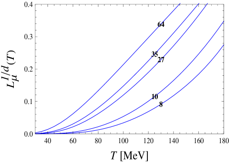
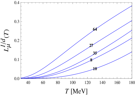
Figure 19: $L_{\mu}^{1/d_{\mu}}(T)$ for the MIT bag model (left panel) and the constituent quark model (right panel). Here $d_{\mu}=C_{2}(\mu)/C_{2}({\bf 3})$, is the ratio of the two body Casimir operator for the irrep $\mu={\bf 8},{\bf 10},{\bf 27},{\bf 35},{\bf 64}$, relative to the fundamental one. We consider gluodynamics and $N_{c}=3$.

In a recent paper Mykkanen et al. (2012) a thorough study establishes the Casimir scaling properties of the Polyakov loop in pure gluodynamics and large $N_{c}$, above the phase transition, and at sufficiently large temperatures. That means that $L_{\mu}^{1/d_{\mu}}(T)$ approaches a $\mu$-independent value at high temperatures. Here $d_{\mu}=C_{2}(\mu)/C_{2}({\bf 3})$, is the ratio of the two body Casimir operator for the irrep $\mu$ relative to the fundamental one. One can see from their calculation that sizable deviations from this scaling behavior take place for lower temperatures. It is interesting to see whether the models studied in the present work comply to this Casimir scaling departures. As we have repeatedly stressed, the low temperature behavior is dominated by the lightest energy gap associated with the screening of heavy sources, and as such, implement different scaling rules. For the case considered in Mykkanen et al. (2012), and combining our results in Fig. 19, we generally agree with the monotonous offset of the Casimir scaling below the phase transition as the dimension of the representation increases, for $\mu={\bf 8}$, ${\bf 10}$, ${\bf 27}$, ${\bf 35}$, and ${\bf 64}$ (albeit with inversions in ${\bf 8}$ and ${\bf 10}$, and in ${\bf 27}$ and ${\bf 35}$ in the constituent quark model). In this regard, it would be interesting to pursue Casimir scaling violations to temperatures below $0.75\,T_{c}$, where the data of Ref. Mykkanen et al. (2012) stop. It is remarkable that, even though Polyakov loops are exponentially suppressed at low temperatures, as established here, lattice calculations may provide a clear signal on the light of Casimir scaling.

VIII Conclusions

In the present paper we have extended a hadronic sum rule for the Polyakov loop developed previously for the fundamental representation to higher representations of the ${\mathrm{SU}}(3)$ gauge group. Quite generally we find that for any irreducible ${\mathrm{SU}}(3)$ representation $\mu$ there is a finite energy gap $\Delta_{\mu}$ which corresponds to the lightest state having an infinitely heavy source transforming according to the irrep $\mu$ screened by a conjugated dynamical charge. This provides the Boltzmann factor controlling the low temperature exponential suppression of the Polyakov loop. While these gaps could in principle be computed on the lattice, they can be compared to existing hadronic physical states to some approximation. Regardless of whether or not these states can be extracted from suitable experiments, they provide a basis for which the completeness of the hadronic spectrum can be tested.

One can alternatively formulate the problem using the Polyakov loop itself as a quantum and local dynamical variable and hence define the corresponding partition function as an integral over $\Omega$ which is proportional to the probability of having a given value of $\Omega$ at a given temperature. We have found a low temperature character expansion which involves group representations with higher dimensionality.

Within an independent particle model picture the hadronic sum rule generates scaling properties at low temperatures which offer an alternative to Casimir scaling and could possibly be tested on the lattice. One good feature of these models is the correct counting of multiparton states. We have found that by analyzing the models within a low temperature expansion an equivalent multipartonic decomposition of the Fock space arises in terms of the number of constituents. The clustering of these states into hadrons turns out to be more tricky, as there is no completely unambiguous way of defining the hadronic partition function. This has to do with the emergence of globally color singlet states which are reducible, i.e. clusters that i) are decomposable into subclusters which are themselves color singlets, ii) can be dissociated with an energy much smaller than the mass of the subclusters, and iii) within the approximation that these states interact through residual spin-flavor forces, they factorize in the partition function. From this point of view, a six quark state such as the deuteron or the weakly bound $X(3872)$ made as a large $c\bar{c}\bar{n}n$ and a small $c\bar{c}$ component would factorize in the partition function sum. On the other hand, some states in this category create sharp resonances which in the standard HRG model are counted on their own, as suggested by the quantum virial expansion analysis Dashen and Rajaraman (1974); Venugopalan and Prakash (1992). By using as an example the MIT bag model, which is free from center of mass corrections due to heavy source, we find very visible consequences of considering all states or just irreducible ones. Therefore, we expect that future lattice calculations may shed some light on this intriguing issue which already shows up in a low temperature expansion.

Saturating the sum rule even to moderate temperatures requires a large number of excited states. This is due to the lack of mass gaps in the spectrum besides the finite and large lowest excitation gaps, $\Delta_{\mu}$, generating by screening static color charges in a given irreducible representation, $\mu$. Thus, even for heavy quarks, relativistic corrections become important for high excitations. Our model calculations implemented relativistic features.

As we have stressed in this paper it is also crucial to maintain at any rate the quantum and local character of the Polyakov loop, as simple-minded mean-field approximations applied to the Polyakov loop in e.g. a PNJL approach washes out all information on higher representations.

As we mentioned in the Introduction, the definition of a hadron as a true or effective elementary degree of freedom from a thermodynamic point of view is subtle. In this regard it is remarkable that lattice calculations for the trace anomaly are reproduced in the bulk and within uncertainties by the Hadron Resonance Gas model taking PDG states Karsch et al. (2003); Borsanyi et al. (2010a); Huovinen and Petreczky (2010); Borsanyi et al. (2013). The partition function actually counts the total number of states at large temperatures. In a previous paper Megias et al. (2012) we profited from the results found in the RQM Godfrey and Isgur (1985); Capstick and Isgur (1986). The extension of these quark model calculations needed for the saturation of our generalized sum rule given by Eq. (7) beyond the fundamental representation remains to be done (for a sketch see e.g. Ruiz Arriola et al. (2013a)). Finally, calculations for tetraquark and pentaquark excited states require assumptions about the color structure of interactions which actually correspond to a specific choice on the interacting forces from the model building point of view. However, the very existence of a hadronic limit imposes non trivial constraints on the microscopic quark and gluon interactions. We hope the present paper will stimulate further developments in setting up a Polyakov spectroscopy exploiting the partition function character of the Polyakov loop in different representations.

Appendix A Counting of irreducible color configurations

In this section we describe the counting of reducible and irreducible color configurations. Results up to three constituents are given in Table 1, and up to four constituents for the fundamental representation in Table 2.

The total multiplicity (adding the number of irreducible plus reducible configurations) can be computed straightforwardly when all spin-flavor states are different. Namely, it suffices to compute the Clebsch-Gordan series of the product of $n_{q}$ ${\bf 3}$’s, $n_{\bar{q}}$ ${\bf\bar{3}}$’s, and $n_{g}$ ${\bf 8}$’s, and count how many times each irrep appears there. For instance

$${\bf 8}\otimes{\bf 8}={\bf 1}\oplus{\bf 8}\oplus{\bf 8}\oplus{\bf 10}\oplus{\bf\bar{10}}\oplus{\bf 27},$$ (133)

implies that the configuration $(0,0,1^{2})$ (two gluons in different spin-flavor states) can “screen” a singlet source (or rather form a singlet) in one way, an adjoint source in two ways, etc. Unfortunately, we do not have such a simple counting when some spin-flavor labels are repeated, nor to separate reducible from irreducible configurations.

We recall that a color configuration is reducible when a non-empty subset of the constituents forms a singlet. This is different from reducibility under the group (minimal subspace). For instance, in the example above the two gluons screening an adjoint source span a space ${\bf 8}\times{\bf 8}$, which is therefore reducible under the group. However, the color configurations are themselves irreducible since a non-empty subset of constituents forming a singlet would make use of the two gluons, and the adjoint source would not be screened (or equivalently, screening the source requires at least one gluon, and the other gluon cannot form a singlet by itself).

In general, we have a certain number of constituents, $q$, ${\bar{q}}$, $g$ in various spin-flavor states, $\alpha$, $\beta$, etc, and color states $i$, $j$, etc. To each such constituent we assign an operator (that can be regarded as a creation operator), $q_{\alpha}^{i}$, $\bar{q}_{\alpha,i}$, or $g_{\alpha,j}^{i}$. The operators $q$ and ${\bar{q}}$ are fermionic and $g$ is bosonic. The matrix $g_{\alpha,j}^{i}$ (with respect to $ij$) is traceless. Let $\alpha_{1},\ldots,\alpha_{n_{q}}$ be the spin-flavor states of the $n_{q}$ quarks in the configuration, and similarly $\beta_{1},\ldots,\beta_{n_{\bar{q}}}$ for antiquarks, and $\gamma_{1},\ldots,\gamma_{n_{g}}$ for gluons. This defines a vector space

$${\cal H}={\rm lin}\big{\{}q_{\alpha_{1}}^{i_{1}}\cdots q_{\alpha_{n_{q}}}^{i_{n_{q}}}{\bar{q}}_{\beta_{1},j_{1}}\cdots{\bar{q}}_{\beta_{n_{\bar{q}}},j_{n_{\bar{q}}}}g_{\gamma_{1},l_{1}}^{k_{1}}\cdots g_{\gamma_{n_{g}},l_{n_{g}}}^{k_{n_{g}}}\big{\}}\,,$$ (134)

where the spin-flavor labels are fixed and the color labels run from 1 to 3. ${\cal H}$ carries a representation of ${\mathrm{SU}}(3)$ which in general will be reducible

$${\cal H}=\bigoplus_{\mu}\left(\bigoplus_{k=1}^{t_{\mu}}{\cal H}_{\mu}^{(k)}\right).$$ (135)

Each ${\cal H}_{\mu}^{(k)}$ carries an irrep $\bar{\mu}$. (Recall that the source is in the irrep $\mu$ and therefore the dynamical particles are in $\bar{\mu}$.) The multiplicity $t_{\mu}$ is the total shown in Table 1 for each irrep $\mu$ and for each configuration of constituents $(\{\alpha_{1}\ldots\alpha_{n_{q}}\},\{\beta_{1}\ldots\beta_{n_{\bar{q}}}\},\{\gamma_{1}\ldots\gamma_{n_{g}}\})$.

Instead of working with the $n_{\mu}$-dimensional spaces ${\cal H}_{\mu}^{(k)}$, it is preferable to work with one-dimensional spaces by coupling the states of ${\cal H}_{\mu}^{(k)}$ to a source in the irrep $\mu$ to form a singlet. In ${\mathrm{SU}}(3)$ an irrep of the type $(n,m)=[n+m,m]$ can be represented by a color tensor $\Omega^{i_{1},\ldots,i_{n}}_{j_{1},\ldots,j_{m}}$ completely symmetric in both upper and in lower indices and traceless (i.e. $\Omega^{k,i_{2},\ldots,i_{n}}_{k,j_{2},\ldots,j_{m}}=0$) Coleman (1988). The components of $\Omega^{i_{1},\ldots,i_{n}}_{j_{1},\ldots,j_{m}}$ are c-numbers. The abovementioned two-gluon configurations $(0,0,1^{2})$ screening the adjoint source in two ways correspond to the two combinations

$$\Omega^{i}_{j}g_{\alpha,k}^{j}g_{\beta,i}^{k},\quad\Omega^{i}_{j}g_{\alpha,i}^{k}g_{\beta,k}^{j}.$$ (136)

These operators are linearly independent and span a two-dimensional space. By changing $\Omega$ (or by applying group rotations with fixed $\Omega$) each operator would generate an 8-dimensional irreducible space. For $(0,0,2)$, i.e. $\alpha=\beta$, the states are no longer linearly independent and the dimension of the spanned space becomes one (the antisymmetric combination disappears).

For an arbitrary irrep $\mu$, because of irreducibility, any choice of $\Omega^{i_{1},\ldots,i_{n}}_{j_{1},\ldots,j_{m}}$ gives equivalent results. The simplest choice is to take only one component different from zero (plus those needed to fulfill the constraints of symmetry and tracelessness).

All operators can be generated by using the appropriate source $\Omega$, the $q$, ${\bar{q}}$, $g$ operators, and contracting all indices. Besides the Kronecker delta, the only invariant tensor that can be used is the $\epsilon_{ijk}$ (or $\epsilon^{ijk}$). Not all operators so obtained will be linearly independent. As noted above, the total dimension of the space is known beforehand when spin-flavor states are all different, so in this case it is easy to check when a sufficient number of independent operators have been accounted for. To go to the case in which some of the spin-flavor states are equal, it is sufficient to take these same operators and identify spin-flavor labels there, and then count the new number of linearly independent operators.

The basis of operators obtained in this way will contain both reducible and irreducible color configurations in general. To separate and then count the two types of configurations the prescription is to identify first the subspace of reducible ones, the “irreducible” subspace being the orthogonal complement.

It is sufficient to consider the case when all spin-flavor states are different. For a given set $(n_{q},n_{\bar{q}},n_{g})$, the construction of the reducible color configurations of type $\mu$ is recursive. First one considers all $\mu$-configurations with a smaller number of constituents and then completes the set by adding all possible non-empty singlet configurations so that the total number of constituents $(n_{q},n_{\bar{q}},n_{g})$ is attained. This procedure produces the subspace of reducible configurations.

Not all reducible states so obtained will be linearly independent. For instance, for pentaquark configurations of the type $(0,1^{4},0)$ screening a fundamental source,

$$(\Omega^{i}{\bar{q}}_{\alpha,i})({\bar{q}}_{\beta,j}{\bar{q}}_{\gamma,k}{\bar{q}}_{\delta,l}\epsilon^{jkl}),$$ (137)

one could expect to form four states by screening the source with either $\alpha$, $\beta$, $\gamma$ or $\delta$, however, just three of them are linearly independent. In the present case the Clebsch-Gordan series is

$${\bf\bar{3}}\otimes{\bf\bar{3}}\otimes{\bf\bar{3}}\otimes{\bf\bar{3}}={\bf\bar{3}}\oplus{\bf\bar{3}}\oplus{\bf\bar{3}}\oplus{\bf 6}\oplus{\bf 6}\oplus{\bf\bar{15}}\oplus{\bf\bar{15}}\oplus{\bf\bar{15}}\oplus{\bf\bar{15^{\prime}}},$$ (138)

therefore the three reducible configurations saturate the series and there are no irreducible states (i.e., $(0+3)$ in Table 2).

For another example, consider the configuration $(0,1,1^{2})$ with Clebsch-Gordan series

$${\bf\bar{3}}\otimes{\bf 8}\otimes{\bf 8}={\bf\bar{3}}\oplus{\bf\bar{3}}\oplus{\bf\bar{3}}\oplus{\bf 6}\oplus\cdots,$$ (139)

so there are three ways to screen a fundamental source:

$$\Omega^{i}{\bar{q}}_{\alpha,i}g_{\beta,j}^{k}g_{\gamma,k}^{j},\quad\Omega^{i}{\bar{q}}_{\alpha,j}g_{\beta,i}^{k}g_{\gamma,k}^{j},\quad\Omega^{i}{\bar{q}}_{\alpha,j}g_{\beta,k}^{j}g_{\gamma,j}^{k},$$ (140)

the first one is reducible and the two last irreducible and they all are linearly independent.

Finally, for a less trivial case consider $(0,1,1^{3})$ screening a fundamental source. The Clebsch-Gordan series produces ten ${\bf\bar{3}}$. The operators one can write down are of the form

$$\Omega^{i}{\bar{q}}_{\alpha,i}g_{\beta,j}^{k}g_{\gamma,k}^{l}g_{\delta,l}^{j},\quad\Omega^{i}{\bar{q}}_{\alpha,j}g_{\beta,i}^{j}g_{\gamma,k}^{l}g_{\delta,l}^{k},\quad\Omega^{i}{\bar{q}}_{\alpha,j}g_{\beta,i}^{k}g_{\gamma,k}^{l}g_{\delta,l}^{j},$$ (141)

plus those obtained by permutation of the gluonic labels. Operators of the two first types are reducible and span a space of dimension five (two from the first type and three more from the second one). The third type produces six states but only five linearly independent ones, that is, one combination (the symmetric one) is actually reducible, and the other five irreducible.

If there are repeated spin-flavor labels, one can apply the above procedure from scratch or instead use previous results obtained for the case of different labels. In the latter case one should be aware that after setting, say $\beta=\alpha$, in the basis obtained for $\beta\not=\alpha$ some states that were previously irreducible can become reducible (that is, linear combination of manifestly reducible ones). So the correct procedure is again to first identify the reducible space, and then compute its orthogonal complement.

Appendix B Further computational details

B.1 Truncation of infinite sums

To deal with the infinite sums over $n$ in $Z_{q,g}^{\prime}(\omega,T^{\prime},T)$, Eq. (100), we simply cut off the sums when the $z^{\prime}$’s become smaller than $\varepsilon=10^{-10}$.

B.2 The function $f_{\frac{3}{4}}(t)$

The function $f_{\frac{3}{4}}(t)$ is defined by the relation

$$\int_{0}^{\infty}f_{\frac{3}{4}}(t)e^{-st}\,dt=e^{-s^{3/4}}.$$ (142)

$f_{\frac{3}{4}}(t)$ is a positive normalized unimodal function which vanishes (with all its derivatives) at $t=0$ and $t=\infty$.

Use of the Bromwich inversion formula allows to express $f_{\frac{3}{4}}(t)$ as

$$f_{\frac{3}{4}}(t)=\int_{0}^{\infty}\frac{dx}{\pi}\cos(tx-\cos(\pi/8)x^{3/4})e^{-\sin(\pi/8)x^{3/4}}.$$ (143)

The integrand is oscillating and we find that making the change of variables $x=y^{4n/3}$ with $n=1$ or $2$ improves the convergence for large and small $x$. We use the integral in the range $0.2\leq t\leq 6$. For larger $t$ a fit is used of the form

$$f_{\frac{3}{4}}(t)\sim 0.4663\frac{1}{t^{2}}-0.4180\frac{1}{t^{3}}+0.8403\frac{1}{t^{4}}\qquad(t>6).$$ (144)

A saddle point approximation in Eq. (142) allows to obtain the small $t$ behavior of the former function, namely,

$$f_{\frac{3}{4}}(t)\underset{t\to 0}{\sim}e^{-\frac{1}{4}\left(\frac{3}{4\,t}\right)^{3}}\,.$$ (145)

On this basis, for small $t$ we use the fit

$$f_{\frac{3}{4}}(t)\sim\exp\left(-\frac{1}{4}\left(\frac{3}{4\,t}\right)^{3}(1-5.401\,t^{2}-10.35\,t^{3}+24.07\,t^{4})\right)\qquad(t<0.2).$$ (146)

B.3 Clebsch-Gordan series

In order to obtain the expansion in Eq. (50) from Eq. (51) one can use the expressions in Eq. (52) and expand in powers of $q$, ${\bar{q}}$ and $g$. The required Clebsch-Gordan series can be obtained by using back and forth the following two sets of equations:

$$\chi_{\bf 1} = 1$$

$$\chi_{{\bf 6}} = \chi_{\bf 3}^{2}-\chi_{\bf 3}^{*}$$

$$\chi_{{\bf 8}} = \chi_{\bf 3}\chi_{\bf 3}^{*}-1$$

$$\chi_{{\bf 10}} = -2\chi_{\bf 3}\chi_{\bf 3}^{*}+\chi_{\bf 3}^{3}+1$$

$$\chi_{{\bf 15}} = \chi_{\bf 3}^{2}\chi_{\bf 3}^{*}-\chi_{\bf 3}-\chi_{\bf 3}^{*2}$$

$$\chi_{\bf 15^{\prime}} = -3\chi_{\bf 3}^{2}\chi_{\bf 3}^{*}+\chi_{\bf 3}^{4}+2\chi_{\bf 3}+\chi_{\bf 3}^{*2}$$

$$\chi_{{\bf 24}} = \chi_{\bf 3}\chi_{\bf 3}^{*3}-2\chi_{\bf 3}^{2}\chi_{\bf 3}^{*}+2\chi_{\bf 3}-\chi_{\bf 3}^{*2}$$

$$\chi_{{\bf 27}} = \chi_{\bf 3}^{2}\chi_{\bf 3}^{*2}-\chi_{\bf 3}^{3}-\chi_{\bf 3}^{*3}$$

$$\chi_{{\bf 35}} = \chi_{\bf 3}^{4}\chi_{\bf 3}^{*}-3\chi_{\bf 3}^{2}\chi_{\bf 3}^{*2}+4\chi_{\bf 3}\chi_{\bf 3}^{*}-\chi_{\bf 3}^{3}+\chi_{\bf 3}^{*3}-1$$

$$\chi_{{\bf 42}} = \chi_{\bf 3}^{3}\chi_{\bf 3}^{*2}+\chi_{\bf 3}^{2}\chi_{\bf 3}^{*}-2\chi_{\bf 3}\chi_{\bf 3}^{*3}-\chi_{\bf 3}^{4}-\chi_{\bf 3}+2\chi_{\bf 3}^{*2}$$

$$\chi_{{\bf 64}} = -2\chi_{\bf 3}^{4}\chi_{\bf 3}^{*}+\chi_{\bf 3}^{3}\chi_{\bf 3}^{*3}+3\chi_{\bf 3}^{2}\chi_{\bf 3}^{*2}-2\chi_{\bf 3}\chi_{\bf 3}^{*4}-5\chi_{\bf 3}\chi_{\bf 3}^{*}$$ (147)

$$+2\chi_{\bf 3}^{3}+2\chi_{\bf 3}^{*3}+1$$

$$1 = \chi_{\bf 1}$$

$$\chi_{\bf 3}^{2} = \chi_{\bf 3}^{*}+\chi_{\bf 6}$$

$$\chi_{\bf 3}^{3} = \chi_{\bf 1}+2\chi_{{\bf 8}}+\chi_{\bf 10}$$

$$\chi_{\bf 3}^{4} = 3\chi_{\bf 3}+2\chi_{\bf 6}^{*}+3\chi_{\bf 15}+\chi_{\bf 15^{\prime}}$$

$$\chi_{\bf 3}\chi_{\bf 3}^{*} = \chi_{\bf 1}+\chi_{{\bf 8}}$$

$$\chi_{\bf 3}^{2}\chi_{\bf 3}^{*} = 2\chi_{\bf 3}+\chi_{\bf 6}^{*}+\chi_{{\bf 15}}$$

$$\chi_{\bf 3}^{3}\chi_{\bf 3}^{*} = 3\chi_{\bf 3}^{*}+3\chi_{\bf 6}+2\chi_{\bf 15}^{*}+\chi_{\bf 24}^{*}$$ (148)

$$\chi_{\bf 3}^{4}\chi_{\bf 3}^{*} = 3\chi_{\bf 1}+8\chi_{\bf 8}+4\chi_{\bf 10}+2\chi_{\bf 10}^{*}+3\chi_{{\bf 27}}+\chi_{\bf 35}$$

$$\chi_{\bf 3}^{2}\chi_{\bf 3}^{*2} = 2\chi_{\bf 1}+4\chi_{\bf 8}+\chi_{\bf 10}+\chi_{\bf 10}^{*}+\chi_{\bf 27}$$

$$\chi_{\bf 3}^{3}\chi_{\bf 3}^{*2} = 6\chi_{\bf 3}+5\chi_{\bf 6}^{*}+6\chi_{\bf 15}+\chi_{\bf 15^{\prime}}+2\chi_{\bf 24}+\chi_{\bf 42}$$

$$\chi_{\bf 3}^{3}\chi_{\bf 3}^{*3} = 6\chi_{\bf 1}+17\chi_{\bf 8}+7\chi_{\bf 10}+7\chi_{\bf 10}^{*}+9\chi_{\bf 27}+2\chi_{{\bf 35}}+2\chi_{\bf 35}^{*}$$

$$+\chi_{\bf 64}$$

Instead of the identities in Eq. (52), one can alternatively expand Eq. (51) in powers of $\Omega$, so that everything is expressed in terms of $\chi_{\bf 3}(\Omega^{n})$, $\chi_{\bf\bar{3}}(\Omega^{n})$, and $\chi_{\bf 8}(\Omega^{n})$. The two latter expressions are reduced to fundamental characters through

$$\chi_{\bf\bar{3}}(\Omega^{n})=\chi_{\bf 3}(\Omega^{-n}),\quad\chi_{\bf 8}(\Omega^{n})=\chi_{\bf 3}(\Omega^{n})\chi_{\bf 3}(\Omega^{-n})-1.$$ (149)

This allows to repeatedly apply the ${\mathrm{SU}}(3)$ identity

$$\Omega^{2}=\chi_{\bf 3}(\Omega)\Omega-\chi_{\bf\bar{3}}(\Omega)+\Omega^{-1},\quad\Omega\in{\mathrm{SU}}(3),$$ (150)

as well as its adjoint one. In this way everything is expressed as a polynomial of the two variables $\chi_{\bf 3}(\Omega)$ and $\chi_{\bf 3}^{*}(\Omega)$ and Eq. (148) applies.

Still another route is to insert $\chi_{\mu}(\Omega)$, express all characters in terms of eigenvalues of $\Omega$ and carry out the integrations by residues.

Appendix C Numerical results for the bag model with selected configurations

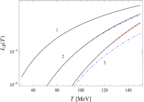
Figure 20: Convergence of the sum over levels for $L_{\bf 3}(T)$ as the cutoff $\Lambda$ is increased. Labels 1, 2, and 3 correspond to sums over configurations with one, two and three constituents, respectively. Dot-dashed, dashed and solid lines correspond to $\Lambda=2$, $3$, and $4\,{\mathrm{GeV}}$, respectively. Convergence is slower for higher temperature and/or a larger numbers of constituents, due to the rapid increase in the number of active configurations.

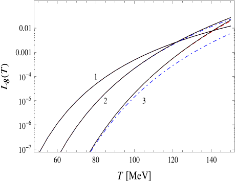
Figure 21: As in Fig. 20 for the adjoint representation.

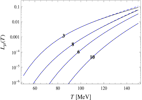
Figure 22: Effect of removing reducible color configurations in $L_{\mu}(T)$ for $\mu={\bf 3}$, ${\bf 8}$, ${\bf 6}$, ${\bf 10}$, and including up to three constituents. Dashed lines: irreducible plus reducible color configurations. Solid lines: irreducible configurations only.

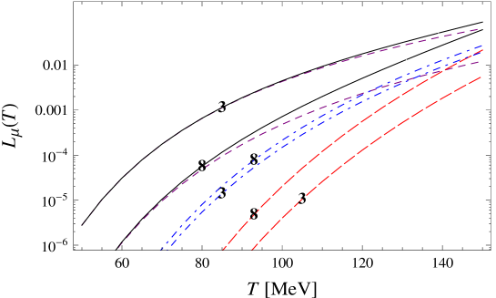
Figure 23: Separate contributions to $L_{\bf 3}$ and $L_{\bf 8}$ from 1 (dashed), 2 (dot-dashed), and 3 (long-dashed) constituents. Solid line: $1+2+3$ constituents.

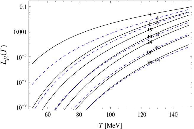
Figure 24: $L_{\mu}(T)$ as a function of the temperature for several irreps and including up to three constituents. For the singlet, $Z_{\bf 1}(T)-1$ is plotted, it includes singlet reducible states.

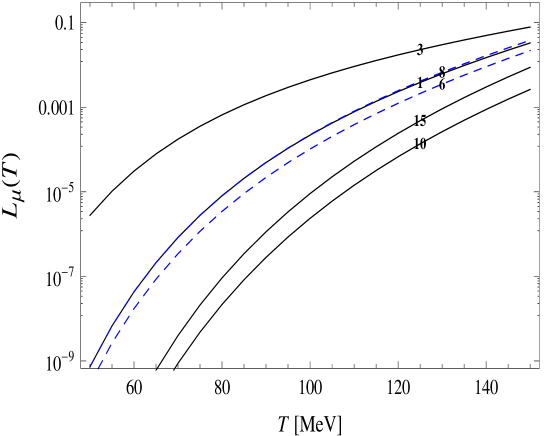
Figure 25: As Fig. 24 but including only quarks and antiquarks. Some irreps are not shown because they are too small for the temperature range.

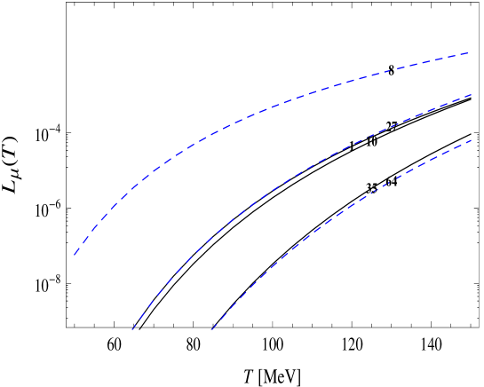
Figure 26: As Fig. 24 but using only gluons.

Numerical results for Sec. V are displayed in Figs. 20, 21, 22, 23, 24, 25, 26 and 27. Lowest bag states are displayed in Tables 4, 5 and 6.

Table 4: Lowest-lying bag one-constituent configurations with their degeneracies for each irrep. “$0+0$” entries have been omitted. $\ell$, $s$, and $g$ stands for light quark ($u,d$), strange quark, and gluon. $n$ $j$ and parity of the constituents are indicated. Irreducible plus reducible degeneracies are displayed.

$\Delta(\,{\mathrm{MeV}})$	config.	1	3	6	8	10	15′	15	24	27	35	42	64
$712.11$	${\bar{\ell}}(1\frac{1}{2}^{-})$		$4+0$
$821.11$	$\bar{s}(1\frac{1}{2}^{-})$		$2+0$
$888.49$	$g(11^{+})$				$3+0$
$998.$	${\bar{\ell}}(1\frac{3}{2}^{+})$		$8+0$
$1107.$	$\bar{s}(1\frac{3}{2}^{+})$		$4+0$
$1136.77$	${\bar{\ell}}(1\frac{1}{2}^{+})$		$4+0$
$1149.85$	$g(12^{-})$				$5+0$
$1245.77$	$\bar{s}(1\frac{1}{2}^{+})$		$2+0$
$1250.26$	${\bar{\ell}}(1\frac{5}{2}^{-})$		$12+0$
$1286.07$	$g(11^{-})$				$3+0$
$1359.26$	$\bar{s}(1\frac{5}{2}^{-})$		$6+0$
$1387.89$	$g(13^{+})$				$7+0$
$1419.04$	${\bar{\ell}}(1\frac{3}{2}^{-})$		$8+0$
$1475.48$	${\bar{\ell}}(2\frac{1}{2}^{-})$		$4+0$
$1482.28$	${\bar{\ell}}(1\frac{7}{2}^{+})$		$16+0$
$1528.04$	$\bar{s}(1\frac{3}{2}^{-})$		$4+0$
$1550.15$	$g(12^{+})$				$5+0$
$1584.48$	$\bar{s}(2\frac{1}{2}^{-})$		$2+0$
$1591.28$	$\bar{s}(1\frac{7}{2}^{+})$		$8+0$
$1609.85$	$g(14^{-})$				$9+0$
$1620.93$	$g(21^{+})$				$3+0$

Table 5: As Table 4 for two-constituent configurations.

$\Delta(\,{\mathrm{MeV}})$	config.	1	3	6	8	10	15′	15	24	27	35	42	64
$1197.62$	$\ell(1\frac{1}{2}^{+})$ $\ell(1\frac{1}{2}^{+})$		$10+0$
$1197.62$	$\ell(1\frac{1}{2}^{+})$ ${\bar{\ell}}(1\frac{1}{2}^{-})$	$0+16$			$16+0$
$1197.62$	${\bar{\ell}}(1\frac{1}{2}^{-})$ ${\bar{\ell}}(1\frac{1}{2}^{-})$			$6+0$
$1306.62$	$\ell(1\frac{1}{2}^{+})$ $s(1\frac{1}{2}^{+})$		$8+0$
$1306.62$	$\ell(1\frac{1}{2}^{+})$ $\bar{s}(1\frac{1}{2}^{-})$	$0+8$			$8+0$
$1306.62$	$s(1\frac{1}{2}^{+})$ ${\bar{\ell}}(1\frac{1}{2}^{-})$	$0+8$			$8+0$
$1306.62$	${\bar{\ell}}(1\frac{1}{2}^{-})$ $\bar{s}(1\frac{1}{2}^{-})$			$8+0$
$1348.67$	$g(11^{+})$ $\ell(1\frac{1}{2}^{+})$			$12+0$
$1348.67$	$g(11^{+})$ ${\bar{\ell}}(1\frac{1}{2}^{-})$		$12+0$					$12+0$
$1415.62$	$s(1\frac{1}{2}^{+})$ $s(1\frac{1}{2}^{+})$		$3+0$
$1415.62$	$s(1\frac{1}{2}^{+})$ $\bar{s}(1\frac{1}{2}^{-})$	$0+4$			$4+0$
$1415.62$	$\bar{s}(1\frac{1}{2}^{-})$ $\bar{s}(1\frac{1}{2}^{-})$			$1+0$
$1444.73$	$\ell(1\frac{1}{2}^{+})$ $\ell(1\frac{3}{2}^{-})$		$32+0$
$1444.73$	$\ell(1\frac{1}{2}^{+})$ ${\bar{\ell}}(1\frac{3}{2}^{+})$	$0+32$			$32+0$
$1444.73$	$\ell(1\frac{3}{2}^{-})$ ${\bar{\ell}}(1\frac{1}{2}^{-})$	$0+32$			$32+0$
$1444.73$	${\bar{\ell}}(1\frac{1}{2}^{-})$ ${\bar{\ell}}(1\frac{3}{2}^{+})$			$32+0$
$1457.67$	$g(11^{+})$ $s(1\frac{1}{2}^{+})$			$6+0$
$1457.67$	$g(11^{+})$ $\bar{s}(1\frac{1}{2}^{-})$		$6+0$					$6+0$
$1494.26$	$g(11^{+})$ $g(11^{+})$	$0+6$			$9+0$	$3+0$				$6+0$
$1553.73$	$s(1\frac{1}{2}^{+})$ $\ell(1\frac{3}{2}^{-})$		$16+0$

Table 6: As Table 4 for three-constituent configurations.

$\Delta(\,{\mathrm{MeV}})$	config.	1	3	6	8	10	15′	15	24	27	35	42	64
$1623.25$	$\ell(1\frac{1}{2}^{+})$ $\ell(1\frac{1}{2}^{+})$ $\ell(1\frac{1}{2}^{+})$	$0+20$			$20+0$
$1623.25$	$\ell(1\frac{1}{2}^{+})$ $\ell(1\frac{1}{2}^{+})$ ${\bar{\ell}}(1\frac{1}{2}^{-})$			$40+0$
$1623.25$	$\ell(1\frac{1}{2}^{+})$ ${\bar{\ell}}(1\frac{1}{2}^{-})$ ${\bar{\ell}}(1\frac{1}{2}^{-})$		$0+64$					$24+0$
$1623.25$	${\bar{\ell}}(1\frac{1}{2}^{-})$ ${\bar{\ell}}(1\frac{1}{2}^{-})$ ${\bar{\ell}}(1\frac{1}{2}^{-})$	$0+20$			$20+0$	$4+0$
$1732.25$	$\ell(1\frac{1}{2}^{+})$ $\ell(1\frac{1}{2}^{+})$ $s(1\frac{1}{2}^{+})$	$0+20$			$32+0$
$1732.25$	$\ell(1\frac{1}{2}^{+})$ $\ell(1\frac{1}{2}^{+})$ $\bar{s}(1\frac{1}{2}^{-})$			$20+0$
$1732.25$	$\ell(1\frac{1}{2}^{+})$ $s(1\frac{1}{2}^{+})$ ${\bar{\ell}}(1\frac{1}{2}^{-})$			$32+0$
$1732.25$	$\ell(1\frac{1}{2}^{+})$ ${\bar{\ell}}(1\frac{1}{2}^{-})$ $\bar{s}(1\frac{1}{2}^{-})$		$0+64$					$32+0$
$1732.25$	$s(1\frac{1}{2}^{+})$ ${\bar{\ell}}(1\frac{1}{2}^{-})$ ${\bar{\ell}}(1\frac{1}{2}^{-})$		$0+32$					$12+0$
$1732.25$	${\bar{\ell}}(1\frac{1}{2}^{-})$ ${\bar{\ell}}(1\frac{1}{2}^{-})$ $\bar{s}(1\frac{1}{2}^{-})$	$0+20$			$32+0$	$12+0$
$1760.63$	$g(11^{+})$ $\ell(1\frac{1}{2}^{+})$ $\ell(1\frac{1}{2}^{+})$		$48+0$					$48+0$	$18+0$
$1760.63$	$g(11^{+})$ $\ell(1\frac{1}{2}^{+})$ ${\bar{\ell}}(1\frac{1}{2}^{-})$	$0+48$			$96+48$	$48+0$				$48+0$
$1760.63$	$g(11^{+})$ ${\bar{\ell}}(1\frac{1}{2}^{-})$ ${\bar{\ell}}(1\frac{1}{2}^{-})$			$48+0$
$1841.25$	$\ell(1\frac{1}{2}^{+})$ $s(1\frac{1}{2}^{+})$ $s(1\frac{1}{2}^{+})$	$0+12$			$16+0$
$1841.25$	$\ell(1\frac{1}{2}^{+})$ $s(1\frac{1}{2}^{+})$ $\bar{s}(1\frac{1}{2}^{-})$			$16+0$
$1841.25$	$\ell(1\frac{1}{2}^{+})$ $\bar{s}(1\frac{1}{2}^{-})$ $\bar{s}(1\frac{1}{2}^{-})$		$0+16$					$4+0$
$1841.25$	$s(1\frac{1}{2}^{+})$ $s(1\frac{1}{2}^{+})$ ${\bar{\ell}}(1\frac{1}{2}^{-})$			$12+0$
$1841.25$	$s(1\frac{1}{2}^{+})$ ${\bar{\ell}}(1\frac{1}{2}^{-})$ $\bar{s}(1\frac{1}{2}^{-})$		$0+32$					$16+0$
$1841.25$	${\bar{\ell}}(1\frac{1}{2}^{-})$ $\bar{s}(1\frac{1}{2}^{-})$ $\bar{s}(1\frac{1}{2}^{-})$	$0+12$			$16+0$	$4+0$
$1848.83$	$\ell(1\frac{1}{2}^{+})$ $\ell(1\frac{1}{2}^{+})$ $\ell(1\frac{3}{2}^{-})$	$0+80$			$128+0$

Figure 27: Cumulative number of states for some irreps.

References

- Shuryak (1978) E. V. Shuryak, Phys.Lett. B78, 150 (1978).
- Meyer-Ortmanns (1996) H. Meyer-Ortmanns, Rev.Mod.Phys. 68, 473 (1996), eprint hep-lat/9608098.
- Harris and Muller (1996) J. W. Harris and B. Muller, Ann.Rev.Nucl.Part.Sci. 46, 71 (1996), eprint hep-ph/9602235.
- Muller and Nagle (2006) B. Muller and J. L. Nagle, Ann.Rev.Nucl.Part.Sci. 56, 93 (2006), eprint nucl-th/0602029.
- Fukushima (2012) K. Fukushima, J.Phys. G39, 013101 (2012), eprint 1108.2939.
- Kogut et al. (1983) J. B. Kogut, M. Stone, H. Wyld, W. Gibbs, J. Shigemitsu, et al., Phys.Rev.Lett. 50, 393 (1983).
- Polonyi et al. (1984) J. Polonyi, H. Wyld, J. Kogut, J. Shigemitsu, and D. Sinclair, Phys.Rev.Lett. 53, 644 (1984).
- Pisarski and Wilczek (1984) R. D. Pisarski and F. Wilczek, Phys.Rev. D29, 338 (1984).
- Aoki et al. (2006) Y. Aoki, G. Endrodi, Z. Fodor, S. Katz, and K. Szabo, Nature 443, 675 (2006), eprint hep-lat/0611014.
- Bazavov et al. (2012) A. Bazavov et al., Phys. Rev. D85, 054503 (2012), eprint 1111.1710.
- Megias et al. (2004) E. Megias, E. Ruiz Arriola, and L. Salcedo, Phys.Rev. D69, 116003 (2004), eprint hep-ph/0312133.
- Braun et al. (2010) J. Braun, H. Gies, and J. M. Pawlowski, Phys.Lett. B684, 262 (2010), eprint 0708.2413.
- Braun et al. (2011) J. Braun, L. M. Haas, F. Marhauser, and J. M. Pawlowski, Phys.Rev.Lett. 106, 022002 (2011), eprint 0908.0008.
- Smith et al. (2013) D. Smith, A. Dumitru, R. Pisarski, and L. von Smekal, Phys.Rev. D88, 054020 (2013), eprint 1307.6339.
- Meisinger and Ogilvie (1996) P. N. Meisinger and M. C. Ogilvie, Phys.Lett. B379, 163 (1996), eprint hep-lat/9512011.
- Fukushima (2004) K. Fukushima, Phys.Lett. B591, 277 (2004), eprint hep-ph/0310121.
- Fodor (2012) Z. Fodor, PTEP 2012, 01A108 (2012).
- Jakovac (2013) A. Jakovac, Phys.Rev. D88, 065012 (2013), eprint 1306.2657.
- Dashen et al. (1969) R. Dashen, S.-K. Ma, and H. J. Bernstein, Phys.Rev. 187, 345 (1969).
- Dashen and Rajaraman (1974) R. Dashen and R. Rajaraman, Phys.Rev. D10, 708 (1974).
- Hagedorn (1985) R. Hagedorn, Lect.Notes Phys. 221, 53 (1985).
- Karsch et al. (2003) F. Karsch, K. Redlich, and A. Tawfik, Phys.Lett. B571, 67 (2003), eprint hep-ph/0306208.
- Borsanyi et al. (2010a) S. Borsanyi, G. Endrodi, Z. Fodor, A. Jakovac, S. D. Katz, et al., JHEP 1011, 077 (2010a), eprint 1007.2580.
- Huovinen and Petreczky (2010) P. Huovinen and P. Petreczky, Nucl.Phys. A837, 26 (2010), eprint 0912.2541.
- Borsanyi et al. (2013) S. Borsanyi, Z. Fodor, C. Hoelbling, S. D. Katz, S. Krieg, Phys.Lett. B730, 99 (2014), eprint 1309.5258.
- Langelage and Philipsen (2010) J. Langelage and O. Philipsen, JHEP 1004, 055 (2010), eprint 1002.1507.
- Ruiz Arriola et al. (2013a) E. Ruiz Arriola, E. Megias, and L. Salcedo, AIP Conf.Proc. 1520, 185 (2013a), eprint 1207.4875.
- Megias et al. (2013a) E. Megias, E. R. Arriola, and L. Salcedo (2013a), eprint 1307.7523.
- Megias et al. (2013b) E. Megias, E. R. Arriola, and L. Salcedo (2013b), eprint 1310.3079.
- Noronha-Hostler et al. (2012) J. Noronha-Hostler, J. Noronha, and C. Greiner, Phys.Rev. C86, 024913 (2012), eprint 1206.5138.
- Endrödi (2013) G. Endrödi, JHEP 1304, 023 (2013), eprint 1301.1307.
- Bali et al. (2013) G. Bali, F. Bruckmann, G. Endrodi, F. Gruber, and A. Schaefer, JHEP 1304, 130 (2013), eprint 1303.1328.
- Cleymans and Redlich (1999) J. Cleymans and K. Redlich, Phys.Rev. C60, 054908 (1999), eprint nucl-th/9903063.
- Begun et al. (2013) V. Begun, M. Gazdzicki, and M. Gorenstein, Phys.Rev. C88, 024902 (2013), eprint 1208.4107.
- Beringer et al. (2012) J. Beringer et al. (Particle Data Group), Phys.Rev. D86, 010001 (2012).
- Arriola et al. (2013) E. R. Arriola, W. Broniowski, and P. Masjuan, Acta Phys.Polon.Supp. 6, 95 (2013), eprint 1210.7153.
- Megias et al. (2012) E. Megias, E. Ruiz Arriola, and L. Salcedo, Phys.Rev.Lett. 109, 151601 (2012), eprint 1204.2424.
- Borsanyi et al. (2010b) S. Borsanyi et al. (Wuppertal-Budapest Collaboration), JHEP 1009, 073 (2010b), eprint 1005.3508.
- Bazavov and Petreczky (2013) A. Bazavov and P. Petreczky (2013), eprint 1301.3943.
- Megias et al. (2006a) E. Megias, E. Ruiz Arriola, and L. Salcedo, Phys.Rev. D74, 065005 (2006a), eprint hep-ph/0412308.
- Megias et al. (2006b) E. Megias, E. Ruiz Arriola, and L. Salcedo, Phys.Rev. D74, 114014 (2006b), eprint hep-ph/0607338.
- Ratti et al. (2006) C. Ratti, M. A. Thaler, and W. Weise, Phys.Rev. D73, 014019 (2006), eprint hep-ph/0506234.
- Sasaki et al. (2007) C. Sasaki, B. Friman, and K. Redlich, Phys.Rev. D75, 074013 (2007), eprint hep-ph/0611147.
- Ciminale et al. (2008) M. Ciminale, R. Gatto, N. D. Ippolito, G. Nardulli, and M. Ruggieri, Phys. Rev. D77, 054023 (2008), eprint 0711.3397.
- Contrera et al. (2008) G. A. Contrera, D. Gomez Dumm, and N. N. Scoccola, Phys. Lett. B661, 113 (2008), eprint 0711.0139.
- Schaefer et al. (2007) B.-J. Schaefer, J. M. Pawlowski, and J. Wambach, Phys. Rev. D76, 074023 (2007), eprint 0704.3234.
- Ghosh et al. (2008) S. K. Ghosh, T. K. Mukherjee, M. G. Mustafa, and R. Ray, Phys.Rev. D77, 094024 (2008), eprint 0710.2790.
- Costa et al. (2009) P. Costa, M. C. Ruivo, C. A. de Sousa, H. Hansen, and W. M. Alberico, Phys. Rev. D79, 116003 (2009), eprint 0807.2134.
- Mao et al. (2010) H. Mao, J. Jin, and M. Huang, J.Phys. G37, 035001 (2010), eprint 0906.1324.
- Sakai et al. (2010) Y. Sakai, T. Sasaki, H. Kouno, and M. Yahiro, Phys. Rev. D82, 076003 (2010), eprint 1006.3648.
- Radzhabov et al. (2011) A. E. Radzhabov, D. Blaschke, M. Buballa, and M. K. Volkov, Phys. Rev. D83, 116004 (2011), eprint 1012.0664.
- Zhang et al. (2010) T. Zhang, T. Brauner, and D. H. Rischke, JHEP 1006, 064 (2010), eprint 1005.2928.
- Megias et al. (2007a) E. Megias, E. Ruiz Arriola, and L. Salcedo, AIP Conf.Proc. 892, 444 (2007a), eprint hep-ph/0610095.
- Megias et al. (2013c) E. Megias, E. Ruiz Arriola, and L. Salcedo, Nucl.Phys.Proc.Suppl. 234, 313 (2013c), eprint 1207.7287.
- Ruiz Arriola et al. (2013b) E. Ruiz Arriola, L. Salcedo, and E. Megias (2013b), eprint 1304.2245.
- Godfrey and Isgur (1985) S. Godfrey and N. Isgur, Phys. Rev. D32, 189 (1985).
- Capstick and Isgur (1986) S. Capstick and N. Isgur, Phys.Rev. D34, 2809 (1986).
- Richard (2010) J. Richard, EPJ Web Conf. 3, 01015 (2010), eprint 1001.5390.
- Vijande et al. (2007) J. Vijande, A. Valcarce, and J.-M. Richard, Phys.Rev. D76, 114013 (2007), eprint 0707.3996.
- Nielsen et al. (2010) M. Nielsen, F. S. Navarra, and S. H. Lee, Phys.Rept. 497, 41 (2010), eprint 0911.1958.
- Carames et al. (2012) T. Carames, A. Valcarce, and J. Vijande, Phys.Lett. B709, 358 (2012), eprint 1203.1123.
- Rajaraman (1979) R. Rajaraman, Mesons in nuclei 1, 197 (1979).
- Gupta et al. (2008) S. Gupta, K. Huebner, and O. Kaczmarek, Phys.Rev. D77, 034503 (2008), eprint 0711.2251.
- Mykkanen et al. (2012) A. Mykkanen, M. Panero, and K. Rummukainen, JHEP 1205, 069 (2012), eprint 1202.2762.
- Tung (1985) W.-K. Tung, Group theory in physics (World Scientific, Singapore, 1985).
- Luscher and Weisz (2002) M. Luscher and P. Weisz, JHEP 0207, 049 (2002), eprint hep-lat/0207003.
- Jahn and Philipsen (2004) O. Jahn and O. Philipsen, Phys.Rev. D70, 074504 (2004), eprint hep-lat/0407042.
- Kogut and Susskind (1975) J. B. Kogut and L. Susskind, Phys.Rev. D11, 395 (1975).
- Polyakov (1980) A. M. Polyakov, Nucl.Phys. B164, 171 (1980).
- Gava and Jengo (1981) E. Gava and R. Jengo, Phys.Lett. B105, 285 (1981).
- Megias et al. (2006c) E. Megias, E. Ruiz Arriola, and L. L. Salcedo, JHEP 01, 073 (2006c), eprint hep-ph/0505215.
- Kaczmarek et al. (2002) O. Kaczmarek, F. Karsch, P. Petreczky, and F. Zantow, Phys.Lett. B543, 41 (2002), eprint hep-lat/0207002.
- Kaczmarek and Zantow (2005) O. Kaczmarek and F. Zantow, Phys. Rev. D71, 114510 (2005), eprint hep-lat/0503017.
- Pisarski (2007) R. D. Pisarski, Prog.Theor.Phys.Suppl. 168, 276 (2007), eprint hep-ph/0612191.
- Megias et al. (2009) E. Megias, E. Ruiz Arriola, and L. Salcedo, Phys.Rev. D80, 056005 (2009), eprint 0903.1060.
- Megias et al. (2010) E. Megias, E. Ruiz Arriola, and L. Salcedo, Phys.Rev. D81, 096009 (2010), eprint 0912.0499.
- Boyd et al. (1996) G. Boyd, J. Engels, F. Karsch, E. Laermann, C. Legeland, et al., Nucl.Phys. B469, 419 (1996), eprint hep-lat/9602007.
- Cheng et al. (2008) M. Cheng, N. Christ, S. Datta, J. van der Heide, C. Jung, et al., Phys.Rev. D77, 014511 (2008), eprint 0710.0354.
- Lucini and Panero (2013) B. Lucini and M. Panero, Phys.Rept. 526, 93 (2013), eprint 1210.4997.
- Megias et al. (2007b) E. Megias, E. Ruiz Arriola, and L. Salcedo, Phys.Rev. D75, 105019 (2007b), eprint hep-ph/0702055.
- Coleman (1988) S. Coleman, Aspects of symmetry (Cambridge University Press, Cambridge, 1988).
- Huang (1987) K. Huang, Statistical mechanics (Wiley, New York, 1987).
- Sasaki and Redlich (2012) C. Sasaki and K. Redlich, Phys.Rev. D86, 014007 (2012), eprint 1204.4330.
- Megias et al. (2006d) E. Megias, E. Ruiz Arriola, and L. Salcedo, PoS JHW2005, 025 (2006d), eprint hep-ph/0511353.
- ’t Hooft (1979) G. ’t Hooft, Nucl.Phys. B153, 141 (1979).
- Polyakov (1978) A. M. Polyakov, Phys.Lett. B72, 477 (1978).
- Susskind (1979) L. Susskind, Phys.Rev. D20, 2610 (1979).
- Dumitru et al. (2004) A. Dumitru, Y. Hatta, J. Lenaghan, K. Orginos, and R. D. Pisarski, Phys.Rev. D70, 034511 (2004), eprint hep-th/0311223.
- Meisinger et al. (2002) P. N. Meisinger, T. R. Miller, and M. C. Ogilvie, Phys.Rev. D65, 034009 (2002), eprint hep-ph/0108009.
- Meisinger et al. (2004) P. N. Meisinger, M. C. Ogilvie, and T. R. Miller, Phys.Lett. B585, 149 (2004), eprint hep-ph/0312272.
- Ruggieri et al. (2012) M. Ruggieri, P. Alba, P. Castorina, S. Plumari, C. Ratti, et al., Phys.Rev. D86, 054007 (2012), eprint 1204.5995.
- Chodos et al. (1974) A. Chodos, R. Jaffe, K. Johnson, C. B. Thorn, and V. Weisskopf, Phys.Rev. D9, 3471 (1974).
- Hasenfratz and Kuti (1978) P. Hasenfratz and J. Kuti, Phys.Rept. 40, 75 (1978).
- Bhaduri (1988) R. K. Bhaduri, Lecture Notes and Supplements in Physics: 22, Addison-Wesly (1988).
- Barnes (1979) T. Barnes, Nucl.Phys. B158, 171 (1979).
- Zouzou and Richard (1994) S. Zouzou and J. Richard, Few Body Syst. 16, 1 (1994), eprint hep-ph/9309303.
- Hagedorn (1965) R. Hagedorn, Nuovo Cim.Suppl. 3, 147 (1965).
- Kapusta (1981) J. I. Kapusta, Phys.Rev. D23, 2444 (1981).
- Venugopalan and Prakash (1992) R. Venugopalan and M. Prakash, Nucl.Phys. A546, 718 (1992).
- Dumitru et al. (2005) A. Dumitru, R. D. Pisarski, and D. Zschiesche, Phys.Rev. D72, 065008 (2005), eprint hep-ph/0505256.
- Megias et al. (2007c) E. Megias, E. Ruiz Arriola, and L. Salcedo, Eur.Phys.J. A31, 553 (2007c), eprint hep-ph/0610163.
- Burnier et al. (2010) Y. Burnier, M. Laine, and M. Vepsalainen, JHEP 1001, 054 (2010), eprint 0911.3480.
- Brambilla et al. (2010) N. Brambilla, J. Ghiglieri, P. Petreczky, and A. Vairo, Phys.Rev. D82, 074019 (2010), eprint 1007.5172.
- Anzai et al. (2010) C. Anzai, Y. Kiyo, and Y. Sumino, Nucl.Phys. B838, 28 (2010), eprint 1004.1562.