Single site model of large N gauge theories coupled to adjoint fermions

Abstract:

We consider a single site large N gauge theory coupled to adjoint fermions at weak coupling. We study the distribution of the eigenvalues of the link variables using a four-dimensional density function. We show that it is possible to recover the infinite-volume continuum limit for a certain range of fermion flavors if we use fermions with a bare mass of zero.

1 Introduction

Large N gauge theory with fermions in the adjoint representation are interesting in many ways. It provides a connection to gravity and string theories [1]. One can use it to understand the transition from conformal to confining field theories [2, 3]. There is a possibility to study continuum gauge theories using a matrix model [4]. In addition, it is possible to numerically investigate a theory with a real number of fermion flavors [5].

The two main questions pertaining to the matrix model are:

1. What is the range of fermion flavors for which the single-site massless theory can be expected to reproduce the infinite-volume continuum theory?

2. Can we reproduce the infinite-volume continuum theory with massive fermions?

We will provide an answer to both these questions in the weak coupling limit and it is a summary of the results presented in [6].

2 Weak coupling analysis and the density function

We refer the reader to [6] for the details of the single site model. The total action depends on $d$ $\operatorname{SU}(N)$ matrices and the gauge transformation is

$$U_{\mu}\to gU_{\mu}g^{\dagger}.$$ (1)

The action has an additional $\operatorname{U}^{d}(1)$ symmetry given by

$$U_{\mu}\to e^{i\alpha_{\mu}}U_{\mu}$$ (2)

with $0\leq\alpha_{\mu}<2\pi$. Restricting $\alpha_{\mu}$ to $\frac{2\pi k_{\mu}}{N}$ with integers $0\leq k_{\mu}<N$ keeps it in $\operatorname{SU}(N)$; otherwise we have trivially extended the $\operatorname{SU}(N)$ theory to a $\operatorname{U}(N)$ theory. Note that the eigenvalues of $U_{\mu}$ are gauge invariant.

In order to figure out if we can reproduce continuum infinite volume results at the level of perturbation theory, we follow [7] and set

$$U_{\mu}=V_{\mu}D_{\mu}V^{\dagger}_{\mu}\,;\ \ \ \ D_{\mu}^{jk}=e^{i\theta^{j}_{\mu}}\delta^{jk}.$$ (3)

We replace the integral over $U_{\mu}$ by an integral over $V_{\mu}$ and $\theta_{\mu}^{j}$. We write $V_{\mu}=e^{ia_{\mu}}$ with $a_{\mu}^{\dagger}=a_{\mu}$ and $a_{\mu}^{ii}=0$ for all $i$ and expand in powers of $a_{\mu}$ to compute observables in perturbation theory. We then have to show that the integral over $\theta_{\mu}^{j}$ is dominated in the large N limit such that continuum infinite volume perturbation theory is reproduced order by order. We restrict ourselves to the lowest order in perturbation theory.

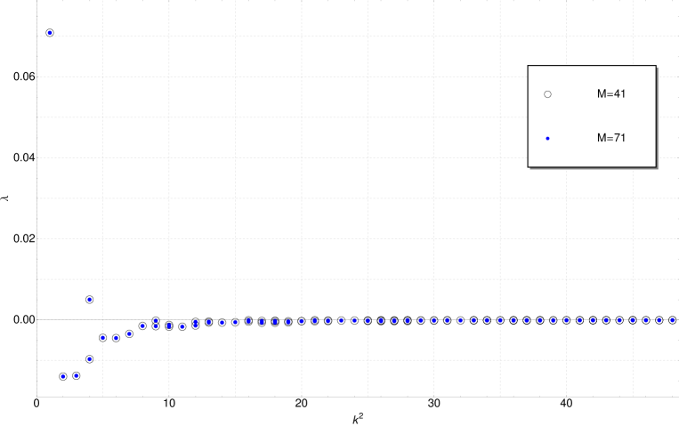
Figure 1: Eigenvalues $\lambda_{k}=\lambda_{k}^{(g)}+f\lambda_{k}^{(o)}$ as a function of $k^{2}$ for the massless overlap Dirac operator with $f=1$ and $m_{w}=-1$ obtained using numerical integration with $M^{4}$ equally spaced points in the four-dimensional integration space.

As $N\to\infty$, we assume that we can define a joint distribution, $\rho(\theta)$, in the following sense: At any finite $N$, for a fixed choice of $\theta_{\mu}^{j}$, $j=1,\ldots,N$ and $\mu=1,\ldots,4$, let

$$\rho(\theta)=\frac{1}{N}\sum_{j}\prod_{\mu}\delta(\theta_{\mu}-\theta_{\mu}^{j})\,;\qquad\qquad\int\prod_{\mu}d\theta_{\mu}\rho(\theta)=1\,,$$ (4)

where $\delta$ denotes the $2\pi$-periodized delta function normalized to $\int_{-\pi}^{\pi}d\theta\delta(\theta)=1$. At the lowest order in perturbation theory (subscripts $g$ and $f$ stand for the gauge and fermion contributions in the equations below),

$$S^{0}_{g,f}[\rho] =N^{2}\mathchoice{{\vbox{\hbox{$\textstyle-$}}\kern-4.86108pt}}{{\vbox{\hbox{$\scriptstyle-$}}\kern-3.25pt}}{{\vbox{\hbox{$\scriptscriptstyle-$}}\kern-2.29166pt}}{{\vbox{\hbox{$\scriptscriptstyle-$}}\kern-1.875pt}}\!\int d^{4}\theta d^{4}\phi\,\rho(\theta)S_{g,f}(\theta-\phi)\rho(\phi)\,;$$ (5)

$$S_{g}(\theta) =-\ln\hat{p}\,;\qquad\hat{p}=\sum_{\mu}4\sin^{2}\frac{\theta_{\mu}}{2}\,;$$ (6)

$$S_{f}(\theta) =2\ln\gamma_{w,o}(m_{w,o})\,;$$ (7)

$$\gamma_{w}(m_{w}) =\left(m_{w}+\frac{\hat{p}}{2}\right)^{2}+\bar{p}\,;\qquad\bar{p}=\sum_{\mu}\sin^{2}\theta_{\mu}\,;$$ (8)

$$\gamma_{o}(m_{o},m_{w}) =\frac{1+m_{o}^{2}}{2}+\frac{1-m_{o}^{2}}{2}\frac{m_{w}+\frac{\hat{p}}{2}}{\sqrt{\gamma_{w}(m_{w})}}\,.$$ (9)

We now assume that, as $N\to\infty$, the partition function will be dominated by a single distribution $\rho(\theta)$, maximizing $S^{0}[\rho]=S^{0}_{g}[\rho]+fS^{0}_{f}[\rho]$ for $f$ flavors of fermions. We will only allow distributions that are non-negative everywhere with the normalization condition in (4). Furthermore, we assume that the dominating distribution $\rho(\theta)$ is smooth and finite for all $\theta$ (in contrast to $\rho$ defined in (4) for angle configurations at finite $N$). Clearly, $S^{0}$ in (9) is invariant under $\rho(\theta)\to\rho(\theta+\alpha)$ for any choice of $\alpha$, corresponding to the invariance under (2).

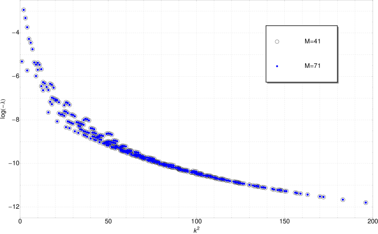
Figure 2: Logarithm of the eigenvalues for the massless overlap Dirac operator with $f=2$ and $m_{w}=-1$ obtained using numerical integration with $M^{4}$ equally spaced points in the four-dimensional integration space.

Owing to the periodic and symmetric nature of $S_{g,f}(\theta)$, it follows that

$$\int_{-\pi}^{\pi}\prod_{\nu}\frac{d\phi_{\nu}}{2\pi}\,S_{g,f}(\theta-\phi)\,e^{i\sum_{\mu}k_{\mu}\phi_{\mu}}=\lambda^{(g,f)}_{k}\,e^{i\sum_{\mu}k_{\mu}\theta_{\mu}}\,;$$ (10)

$$\lambda^{(g,f)}_{k}= \int_{0}^{\pi}\prod_{\nu}\frac{d\phi_{\nu}}{\pi}\,S_{g,f}(\phi)\prod_{\mu}\cos(k_{\mu}\phi_{\mu})\,.$$ (11)

Therefore, Fourier expanding

$$\rho(\theta)=\frac{1}{(2\pi)^{4}}\sum_{k}c_{k}e^{i\sum_{\mu}k_{\mu}\theta_{\mu}}\qquad\textnormal{with}\qquad c_{-k}=c_{k}^{\ast}\,,\quad c_{0}=1$$ (12)

results in

$$S^{0}_{g,f}=N^{2}\sum_{k}c_{k}c_{k}^{\ast}\lambda_{k}^{(g,f)}.$$ (13)

If all the eigenvalues,

$$\lambda_{k}=\lambda^{(g)}_{k}+f\lambda^{(f)}_{k}$$ (14)

for $k\neq 0$ are smaller than zero, the constant mode, $\rho(\theta)=\frac{1}{(2\pi)^{4}}$, will dominate in the large-$N$ limit (i.e., $c_{k}\to 0$ for $k\neq 0$) and the single-site model will be in the correct continuum phase and possibly reproduce the infinite-volume continuum theory.

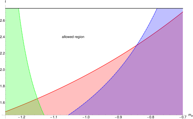
Figure 3: Boundary of the allowed region in the $(m_{w},f)$-plane for massless overlap fermions ($m_{o}=0$). The different lines show $-\lambda^{(g)}_{k}/\lambda^{(o)}_{k}$ for $k=(2,2,2,2)$ (green, dashed), $k=(1,0,0,0)$ (red, solid), and $k=(2,0,0,0)$ (blue, dot-dashed). The intersection points are at $(m_{w},f)\approx(-0.843,2.30)$ and $(m_{w},f)\approx(-1.15,1.65)$.

If some of the eigenvalues are larger than zero, then the action $S^{0}$ in (9) will not be maximized by $\rho(\theta)=\frac{1}{(2\pi)^{4}}$ and some $c_{k}$ ($k\neq 0$) will be non-zero. Since the action in (13) is quadratic, the maximum will be obtained at the boundary of the domain of allowed values for the $c_{k}$’s, which is determined by the condition $\rho(\theta)\geq 0$ for all $\theta$. Therefore, $S[\rho]$ will be maximized by a $\rho(\theta)$ which is zero at least at one point in the four-dimensional Brillouin zone. Due to the shift-invariance, there will then be a class of densities, related by $\rho(\theta)\to\rho(\theta+\alpha)$ with arbitrary $\alpha$, having identical maximum action resulting in a spontaneous breaking of the $\operatorname{U}^{d}(1)$ symmetry in (2).

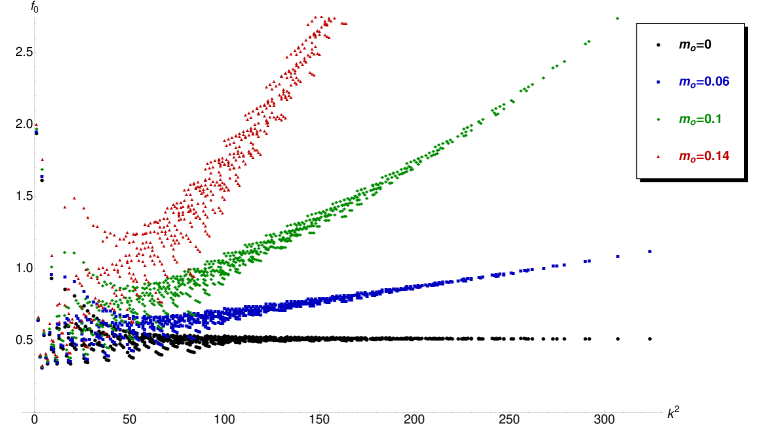
Figure 4: Plots of $f_{0}\equiv-\lambda^{(g)}_{k}/\lambda^{(o)}_{k}$ (for $k_{\mu}\leq 9$) at $m_{w}=-1$ and different choices for $m_{o}$. For $m_{o}=0$, $f_{0}\to 0.5$ as $k^{2}\to\infty$; for all $m_{o}>0$, $f_{0}\to\infty$ as $k^{2}\to\infty$. The boundary of the allowed region is determined by $\max_{k}f_{0}(k)$.

3 Investigation of the allowed regions

We only consider the case of overlap fermions and refer the reader to [6] for the case of Wilson fermions. A sample plot is shown in Fig. 1 where we have computed the eigenvalues $\lambda_{k}=\lambda_{k}^{(g)}+f\lambda_{k}^{(o)}$ for massless overlap fermions with $f=1$ and $m_{w}=-1$. The results are obtained with $M^{4}$ equally spaced points in the four-dimensional integration space and we used $M=41$ and $M=71$ to show that we have reached the limit of the continuum integral. Since two eigenvalues are positive, $(f=1,m_{o}=0,m_{w}=-1)$ is not a point in the allowed region for overlap fermions.

As a second example, we set $f=2$, keeping $m_{o}=0$ and $m_{w}=-1$. In this case, we find all eigenvalues $\lambda_{k}$ to be negative, making this a point inside the allowed region. In Fig. 2, we have plotted $\ln(-\lambda_{k})$ as a function of $k^{2}$ to show that even in the log-scale we have a good estimate for the continuum integral.

Numerically, we find that $\lambda_{k}^{(g)}>0$ for all $k$, which means that a point $(f,m_{o},m_{w})$ will be inside the allowed region (defined by $\lambda_{k}=\lambda_{k}^{(g)}+f\lambda_{k}^{(o)}<0$ for all $k$) iff

1. $\lambda_{k}^{(o)}(m_{o},m_{w})<0$ for all $k$,

2. $f>\max_{k}\left\{-\lambda^{(g)}_{k}/\lambda^{(o)}_{k}\right\}$.

For massless overlap fermions, $-\lambda^{(g)}_{k}/\lambda^{(o)}_{k}\to\frac{1}{2}$ as $k\to\infty$ for all $m_{w}<0$. Therefore, for $m_{o}=0$, the allowed region in the $(m_{w},f)$-plane is determined by eigenvalues $\lambda_{k}$ with $k$ being small. A plot of the boundary of the allowed region in the $(m_{w},f)$-plane for $m_{o}=0$ is shown in Fig. 3.

For $m_{o}>0$, $\lambda_{k}^{(o)}(m_{o})/\lambda_{k}^{(o)}(m_{o}=0)\to 0$ as $k\to\infty$. Together with our results for the massless case, this immediately implies that $-\lambda^{(g)}_{k}/\lambda^{(o)}_{k}\to\infty$ as $k\to\infty$ (see Fig. 4 for numerical results). Therefore, it is necessary to keep $m_{0}=0$ in the weak-coupling limit.

4 Conclusions

Previous numerical work considered quantities like $\operatorname{Tr}U_{\mu}$, $\operatorname{Tr}U_{\mu}U_{\nu}$, $\operatorname{Tr}U_{\mu}U_{\mu}^{\dagger}$ and a few others. These correspond to a select set of values of $k_{\mu}$ in the weak coupling limit. We have shown that this can lead to incorrect conclusions about the validity of the single site model. Since some coefficients with small $k$ could be accidentally small, even looking at $k_{μ}=(1,-1,0,0)$ might not be sufficient to check if the single site model can reproduce the infinite volume continuum theory. Much of the previous numerical work has been done at finite values of the lattice coupling. Even if there is some evidence for an infinite volume limit at finite lattice coupling, the results here show that one cannot take the weak coupling limit. This also applies to numerical work done with massive fermions.

References

- [1] O. Aharony, S. S. Gubser, J. M. Maldacena, H. Ooguri and Y. Oz, Phys. Rept. 323, 183 (2000) [hep-th/9905111].
- [2] A. Patella, L. Del Debbio, B. Lucini, C. Pica and A. Rago, PoS LATTICE 2011, 084 (2011) [arXiv:1111.4672 [hep-lat]].
- [3] A. J. Hietanen, J. Rantaharju, K. Rummukainen and K. Tuominen, JHEP 0905, 025 (2009) [arXiv:0812.1467 [hep-lat]].
- [4] P. Kovtun, M. Unsal, L. G. Yaffe, JHEP 0706, 019 (2007). [hep-th/0702021 [HEP-TH]].
- [5] A. Hietanen, R. Narayanan, JHEP 1001, 079 (2010). [arXiv:0911.2449 [hep-lat]].
- [6] R. Lohmayer and R. Narayanan, Phys. Rev. D 87, 125024 (2013) [arXiv:1305.1279 [hep-lat]].
- [7] G. Bhanot, U. M. Heller and H. Neuberger, Phys. Lett. B 113, 47 (1982).