Zeros of QCD partition function from finite density lattices

Abstract:

Partition function zeros steer the critical behavior of a system. Studying four-flavor lattice QCD at finite temperature and density with the Wilson-clover fermion action and the Iwasaki gauge action using a phase-quenched fermion determinant, we combine statistics from multiple chemical potentials to improve sampling of the configuration space, and aim at unraveling the movement of zeros in finite systems. Preparing for further investigations, we discuss methods and criteria used to sieve through complex parameter space spanned by $(\operatorname{Re}\mu,\,\operatorname{Im}\mu)$ and $(\operatorname{Re}\mu,\,\operatorname{Im}\beta)$, and present statistically robust zeros of the partition function.

1 Introduction

Analyses of partition function zeros may pave the way to the critical point of QCD at finite temperature and density [1, 2]—if executed with care [3]. Danger lurks in the thermodynamic limit with finite statistics, where zeros would appear on the real axis, a manifestation of the “sign problem”. With sufficient statistics, however, we can investigate unimpaired zeros of finite systems and infer the thermodynamic limit.

We study the finite temperature and density ensembles generated with a phase-quenched fermion determinant [4], using four fermion flavors of the Wilson-clover action and the Iwasaki gauge action. Reweighting from simulations at multiple $\mu$ values, we locate zeros of the partition function. We present methods and criteria for a statistically robust zero from combined simulations, and discuss our results.

2 Ensembles and reweighting

We use multi-ensemble reweighting [5] to combine ensembles with various chemical potentials, $\mu$, at two combinations of the bare lattice coupling and the inverse quark mass, $(\beta,\,\kappa)=(1.60,\,0.1371)$ and $(1.58,\,0.1385)$, with lattices of a temporal length, $N_{t}=4$, and spatial volumes, $V=6^{3}$, $6\cdot 6\cdot 8$, $6\cdot 8\cdot 8$, $8^{3}$, and $10^{3}$ (only at the stronger coupling). To maximize the overlap and reduce the reweighting noise, we employ ensembles with $\mu$ values close to the transition/cross-over region, listed in Table 1. We compute action differences due to changing $\mu$ using the first four terms from the Taylor expansion of the logarithm of the fermion determinant with respect to $\mu/T$. Allton et al. [6] implemented $\mu$-reweighting from zero density ensembles, whereas we reweight from multiple ensembles simulated at values of $\mu$ that are close to the region of interest.

$V$	$\mu=0.2$	$0.205$	$0.21$		$V$	$\mu=0.13$	$0.14$	$0.15$	$0.16$
$6^{3}$	16000	16000	16000		$6^{3}$	5000	5000	5000	5000
$6\cdot 6\cdot 8$		32000			$6\cdot 6\cdot 8$	5000	5000	5000	5000
$6\cdot 8\cdot 8$		90000			$6\cdot 8\cdot 8$	5000	13000	13000
$8^{3}$	90000	120000	90000		$8^{3}$	27500	27500	27500
					$10^{3}$		34780	34280	11390

Table 1: Number of configurations used in multi-ensemble reweighting for $(\beta,\,\kappa)=(1.60,\,0.1371)$ on the left and $(\beta,\,\kappa)=(1.58,\,0.1385)$ on the right.

Reweighting results from these ensembles near transition/cross-over region reproduce phase-reweighting only results from ensembles simulated at other $\mu$ values. Shown in Figure 1, at each simulation point with $(\beta,\,\kappa)=(1.60,\,0.1371)$ and $V=8^{3}$, the phase-reweighted quark number density deviates within the statistical uncertainty from the multi-ensemble $\mu$-reweighted value.

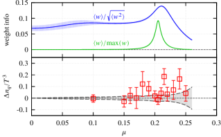
Figure 1: The lower panel shows, for $(\beta,\,\kappa)=(1.60,\,0.1371)$ with $V=8^{3}$, the quark number density from each ensemble subtracted by the multi-ensemble ($\mu=0.2$, $0.205$, and $0.21$) reweighted value, with the reweighted standard deviation shown as the gray band. The upper panel shows the weight statistics, with the partially indiscernible shadow band representing the corresponding standard deviation, where $w$ represents the real part of the weight and $\langle\cdot\rangle$ indicates multi-ensemble average.

3 Partition function zeros and reliability

For a finite system simulated with real parameters, zeros of the partition function manifest themselves in the vanishing of both real and imaginary parts of the average weight from reweighting with complex parameters. In practice, by reweighting with a real parameter, $p$, and an imaginary part of some parameter, $q$, we minimize the squared absolute value of a ratio of total weights, $w$,

$$\mathcal{Z}_{\text{norm}}=\frac{\sum_{U}w(p,\,iq;\,U)}{\sum_{U}w(p,\,iq=0;\,U)}\,,\quad\text{where $\textstyle\sum_{U}$ is over all configurations.}$$ (1)

It is effectively a ratio of partition functions with excessive oscillating terms removed.

In this paper, we report on zeros of partition functions in the parameter space of $(p,\,q)$ being either $(\operatorname{Re}\mu,\,\operatorname{Im}\mu)$ or $(\operatorname{Re}\mu,\,\operatorname{Im}\beta)$.

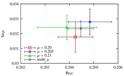
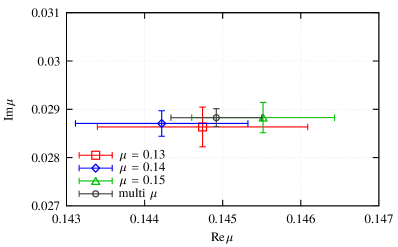
Figure 2: Location of the first partition function zero with $V=8^{3}$. Shown in the left panel is $(\beta,\,\kappa)=(1.60,\,0.1371)$; the right panel $(\beta,\,\kappa)=(1.58,\,0.1385)$.

We observe consistency across results from reweighting of a single ensemble and multiple ensembles. Figure 2 compares multi-ensemble reweighting to single-ensemble reweighting in the complex $\mu$ plane. Combining three ensembles achieves more than a $40\%$ reduction in statistical uncertainties.

To assess the numerical reliability of the partition function zeros, we seek constraint from the uncertainty of the partition function with a complex parameter, $x$, reweighted from $x_{0}$,

$$\mathcal{Z}^{\prime}\approx\int\operatorname{d\!}Oe^{O(x-x_{0})}\operatorname{Prob}_{0}[O]=\frac{1}{\mathcal{Z}_{0}}\int\operatorname{d\!}Ue^{-S_{0}+O_{0}(x-x_{0})}\,,$$ (2)

where the observable $O=-\frac{\partial S}{\partial x}$, with $\operatorname{Prob}_{0}[O]$ the distribution of $O$ at $x_{0}$. It approximates the partition function up to the first derivative of the action, though the relation using $\beta$ is exact [7]. Away from real zeros generated by two approximately Gaussian peaks, with $L$ independent and identically distributed configurations, we derive the confidence region, $|x-x_{0}|$, satisfying $|\mathcal{Z}^{\prime}|>k\sigma(|\mathcal{Z}^{\prime}|)$,

$$\sum_{j}\left|x_{j}-x_{j,0}\right|^{2}\sigma^{2}(O_{j})<\ln\Big{[}\Big{(}\frac{L}{k^{2}}+1\Big{)}\big{/}2\Big{]}\,,$$ (3)

where $\sigma^{2}(O_{j})$ is the variance of a single peak of its distribution, with $x_{j}$ denoting multiple parameters.

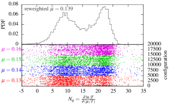
Figure 3: Distribution of quark number, $N_{q}=\frac{\partial\ln\mathcal{Z}}{\partial(\mu/T)}$, for $(\beta,\,\kappa)=(1.58,\,0.1385)$ with $V=6^{3}$. Top panel shows the histogram at $\mu=0.139$ by reweighting from all configurations shown in the bottom.

For $\mu$-reweighting, we look at the reweighted probability distribution function of the quark number, $N_{q}=\frac{\partial\ln\mathcal{Z}}{\partial(\mu/T)}$, and estimate its width. Figure 3 shows an example for $(\beta,\,\kappa)=(1.58,\,0.1385)$ with $V=6^{3}$. The bottom panel is a scatter plot of the measured value with restored phase from complex weight $w$, by multiplying $\frac{w}{\operatorname{Re}w}$ for each configuration. These four ensembles contribute to the reweighted histogram in the upper panel, from which we estimate the width of a single peak, $\sigma(N_{q})=2.5(3)$, at $\mu=0.139$, assuming two Gaussian peaks with approximately equal widths.

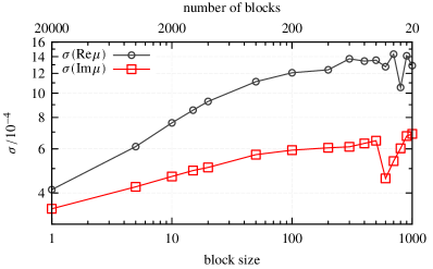
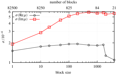
Figure 4: Estimated standard deviation against block size, for the location of the first partition function zero at $(\beta,\,\kappa)=(1.58,\,0.1385)$, with $V=6^{3}$ on the left and $8^{3}$ on the right. Both axes are in logarithmic scales.

To estimate the number of independent configurations with minimum effect of autocorrelation, we investigate the block size effects on the jackknife estimated standard deviation of the location of the first partition function zero away from the real axis. Blocking saturates the estimated standard deviation after increasing the block size up to about $100$, both for $20,000$ configurations for $V=6^{3}$ from four ensembles, and for $82,500$ configurations for $V=8^{3}$ from three ensembles, shown in Figure 4. The estimated error oscillates within about $10\%$, with increasing block sizes. Unreliable estimations seem to occur when the number of blocks becomes $\lesssim 40$; we hence choose statistical errors estimated by jackknife with a block size of $50$.

We estimate the number of independent configurations as the total configuration number divided by $100(20)$ (considering $20\%$ error) following the above observation. For the parameter set, $(\beta,\,\kappa)=(1.58,\,0.1385)$, with $V=6^{3}$, we have an independent sample size, $L\sim 200(40)$. For a determination of $|\mathcal{Z}_{\text{norm}}|$ larger than three times of its standard deviation, $k=3$, applying Eq. (3), we get the confidence region with $|\Delta\mu|<0.16(2)$.

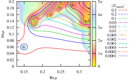
Figure 5: $|\mathcal{Z}_{\text{norm}}|$ and its standard deviation as a color map, at $(\beta,\,\kappa)=(1.58,\,0.1385)$, with $V=6^{3}$.

We compare the estimated confidence radius with the statistical uncertainty of $|\mathcal{Z}_{\text{norm}}|$, from the jackknife method using the actual data. As an example for $(\beta,\,\kappa)=(1.58,\,0.1385)$ with $V=6^{3}$, we compute $|\mathcal{Z}_{\text{norm}}|$ on a grid of the complex $\mu$ plane, with the grid spacing $\delta\mu=0.002$. Figure 5 shows contours of $|\mathcal{Z}_{\text{norm}}|$, with visible isolated zeros, which should be expected from an analytic function. The color map shows the relative size of the absolute value with respect to its standard deviation, on a scale from $0$ to $5\,\sigma$, with the pure white color denoting $|\mathcal{Z}_{\text{norm}}|>5\,\sigma$. In the right side of the figure, where no real zeros of partition function from two approximated Gaussian states would be expected, the cyan $3\,\sigma$ region is slightly larger than the edge of the confidence radius from Gaussian approximation, $|\Delta\mu|=0.16(2)$, centering at $\mu=0.139$. This is probably caused by the approximation of the partition function. The confidence radius excludes the area where statistical noise is too large to reliably estimate $|\mathcal{Z}_{\text{norm}}|$, and zeros located near or outside of the radius are mostly likely to be either spurious ones or affected by noise.

Zeros within the confidence radius, on the other hand, are from the cancellation of two states with high reliabilities. The first zero away from the real axis in Figure 5 is clearly a good signal, since it is away from the boundary of our estimated confidence region, and all values surrounding this zero is determined at more than $5\,\sigma$ level. The second and third one, being very close to each other, require greater care to properly interpret their meaning. We observe that, (a) values between these two are badly estimated $|\mathcal{Z}_{\text{norm}}|<\sigma$, (b) some of the jackknife blocks contain only one zero in that region, and (c) their locations differ within statistical uncertainties estimated by the jackknife method. We thus consider only the lower one as the real zero and the higher one of these two as spurious.

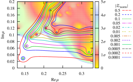
Figure 6: $|\mathcal{Z}_{\text{norm}}|$ and its standard deviation as a color map, at $(\beta,\,\kappa)=(1.58,\,0.1385)$, with $V=8^{3}$.

As a further example to compare with the results from $V=6^{3}$, we show the results from $V=8^{3}$ in Figure 6. With increasing volume, the confidence region inferred from the color map shrinks compared to Figure 5, and more spurious-zero suspects can be seen. Zeros, on the other hand, are also closer to the real axis. We can reliably determine the first two zeros, as $|\mathcal{Z}_{\text{norm}}|$ surrounding them are nonzero with a confidence of more than $5\,\sigma$.

We use Jackknife estimated uncertainties of zero locations in our analysis, as they are consistent with the approximated confidence region and offer a cross-check for the reliability of zero locations.

We also apply the above technique to zeros of partition functions obtained with the real valued $\mu$ and the imaginary part of $\beta$.

4 Results and discussions

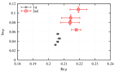
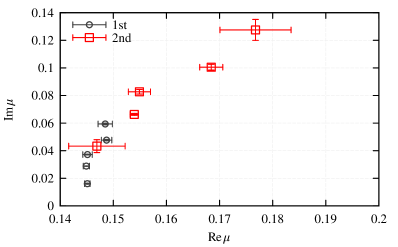
Figure 7: First and second zeros of partition functions in the plane of a complex valued $\mu$, with $(\beta,\,\kappa)=(1.60,\,0.1371)$ on the left and $(\beta,\,\kappa)=(1.58,\,0.1385)$ on the right. Same colored symbols are from $V=6^{3}$, $6\cdot 6\cdot 8$, $6\cdot 8\cdot 8$, $8^{3}$, and $10^{3}$ (right panel only), counting from top to bottom.

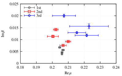
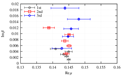
Figure 8: First three zeros of partition functions in the plane of a real valued $\mu$ and the imaginary part of $\beta$, with $(\operatorname{Re}\beta,\,\kappa)=(1.60,\,0.1371)$ on the left and $(\operatorname{Re}\beta,\,\kappa)=(1.58,\,0.1385)$ on the right. Same colored symbols are from $V=6^{3}$, $6\cdot 6\cdot 8$, $6\cdot 8\cdot 8$, $8^{3}$, and $10^{3}$ (right panel only), counting from top to bottom.

We present results of partition function zeros from $\mu$ reweighting with additional imaginary part of $\mu$ or imaginary part of $\beta$. Figure 7 and 8 shows zero locations in the complex $\mu$ plane and in the real $\mu$ and imaginary $\beta$ plane, respectively.

Despite more ensembles with $(\beta,\,\kappa)=(1.60,\,0.1371)$, zeros with $(\beta,\,\kappa)=(1.58,\,0.1385)$ possess smaller uncertainties. This is likely due to larger phase factors of the fermion determinant at the stronger coupling, which goes through a transition at smaller $\mu/T$. In addition, zeros at the stronger coupling appear to align on a single curve, contrasting with zeros spread out more at the weaker coupling. This behavior may indicate better statistics at the stronger coupling, or may suggest a feature of zero locations for the system enters a regime of a strong first-order transition.

We will analyze zero behaviors in a separate detailed report soon.

- [1] Z. Fodor and S. Katz, Lattice determination of the critical point of QCD at finite T and mu, JHEP 03 (2002) 014, [hep-lat/0106002].
- [2] Z. Fodor and S. Katz, Critical point of QCD at finite T and mu, lattice results for physical quark masses, JHEP 0404 (2004) 050, [hep-lat/0402006].
- [3] S. Ejiri, Lee-Yang zero analysis for the study of QCD phase structure, Phys.Rev. D73 (2006) 054502, [hep-lat/0506023].
- [4] X.-Y. Jin, Y. Kuramashi, Y. Nakamura, S. Takeda, and A. Ukawa, Finite size scaling study of finite density QCD on the lattice, arXiv:1307.7205.
- [5] A. M. Ferrenberg and R. H. Swendsen, Optimized Monte Carlo analysis, Phys.Rev.Lett. 63 (1989) 1195–1198.
- [6] C. Allton, M. Doring, S. Ejiri, S. Hands, O. Kaczmarek, et al., Thermodynamics of two flavor QCD to sixth order in quark chemical potential, Phys.Rev. D71 (2005) 054508, [hep-lat/0501030].
- [7] N. A. Alves, B. A. Berg, and S. Sanielevici, Spectral density study of the SU(3) deconfining phase transition, Nucl.Phys. B376 (1992) 218–252, [hep-lat/9107002].