Impacts of high dimensionality in finite samples

Abstract

High-dimensional data sets are commonly collected in many contemporary applications arising in various fields of scientific research. We present two views of finite samples in high dimensions: a probabilistic one and a nonprobabilistic one. With the probabilistic view, we establish the concentration property and robust spark bound for large random design matrix generated from elliptical distributions, with the former related to the sure screening property and the latter related to sparse model identifiability. An interesting concentration phenomenon in high dimensions is revealed. With the nonprobabilistic view, we derive general bounds on dimensionality with some distance constraint on sparse models. These results provide new insights into the impacts of high dimensionality in finite samples.

T1Supported by NSF CAREER Award DMS-09-55316 and Grant DMS-08-06030.

1 Introduction

Thanks to the advances of information technologies, large-scale data sets with a large number of variables or dimensions are commonly collected in many contemporary applications that arise in different fields of sciences, engineering and humanities. Examples include marketing data in business, panel data in economics and finance, genomics data in heath sciences, and brain imaging data in neuroscience, among many others. The emergence of a large amount of information contained in high-dimensional data sets provides opportunities, as well as unprecedented challenges, for developing new statistical methods and theory. See, for example, Hall (2006) and Fan and Li (2006) for insights and discussions on the statistical challenges associated with high dimensionality, and Fan and Lv (2010) for a brief review of some recent developments in high-dimensional sparse modeling with variable selection. The approach of variable selection aims to effectively identify important variables and efficiently estimate their effects on a response variable of interest.

For the purpose of prediction and variable selection, it is important to understand and characterize the impacts of high dimensionality in finite samples. Hall, Marron and Neeman (2005) investigated this problem under the asymptotic framework of fixed sample size $n$ and diverging dimensionality $p$, and revealed an interesting geometric representation of high dimension, low sample size data. When viewed in the diverging $p$-dimensional Euclidean space, the randomness in the data vectors can be asymptotically squeezed into random rotation, with the shape of the rescaled $n$-polyhedron approaching deterministic, modulo the orientation. Such concentration phenomenon of random design matrix in high dimensions is also shared by the concentration property in Fan and Lv (2008) (see Definition 1), in the asymptotic setting of both $n$ and $p$ diverging. Geometrically, this property means that the configuration of the $n$ sub-data vectors, modulo the orientation, becomes close to regular asymptotically. Such a property is key to establishing the sure screening property, which means that all important variables are retained in the reduced feature space with asymptotic probability one, of the sure independence screening (SIS) method introduced in Fan and Lv (2008).

The SIS uses the idea of independence learning by applying componentwise regression. Techniques of independence learning have been widely used for variable ranking and screening. Recent work on variable screening includes Fan and Fan (2008), Hall, Titterington and Xue (2009), Fan, Feng and Song (2011), Xue and Zou (2011), Zhu et al. (2011), Delaigle and Hall (2012), Li, Zhong and Zhu (2012), Mai and Zou (2013) and Bühlmann and Mandozzi (2012), among others. The utility of these methods is characterized by the sure screening property. In particular, Fan and Lv (2008) proved that the concentration property holds when the design matrix is generated from Gaussian distribution, and conjectured that it may well hold for a wide class of elliptical distributions. Samworth (2008) presented some simulation studies investigating such a property for non-Gaussian distributions. The first major contribution of our paper is to provide an affirmative answer to the conjecture posed in Fan and Lv (2008).

To ensure model identifiability and stability for reliable prediction and variable selection, it is practically important to control the collinearity for sparse models. Since it is well known that the level of collinearity among covariates typically increases with the model dimensionality, bounding the sparse model size can be effective in controlling model collinearity. Such a bound is characterized by the concept of robust spark (see Definition 2). Another contribution of the paper is to establish a lower bound on the robust spark in the setting of large random design matrix generated from the family of elliptical distributions.

In addition to the above probabilistic view of finite samples in high dimensions, we also present a nonprobabilistic high-dimensional geometric view. Both views are concerned with how much information finite sample contains. A fundamental question is what the impact of high dimensionality on differentiating the subspaces spanned by different sets of predictors is. Such a question is tied to the issue of model identifiability. In this paper, we intend to derive general bounds on dimensionality with some distance constraint on sparse models.

The rest of the paper is organized as follows. Section 2 establishes the concentration property and robust spark bound for large random design matrix generated from elliptical distributions. We investigate general bounds on dimensionality with distance constraint from a nonprobabilistic point of view in Section 3. Section 4 presents two numerical examples to illustrate the theoretical results. We provide some discussions of our results and their implications in Section 5. All technical details are relegated to the Appendix.

2 Concentration property and robust spark bound of large random design matrix

In this section, we focus on the case of large random design matrix observed in a high-dimensional problem, in which each column vector contains the information of a particular covariate. In high-dimensional sparse modeling, a common practice is to assume that only a faction of all covariates, the so-called true or important covariates, contribute to the regression or classification problem, whereas the other covariates, the so-called noise covariates, are simply noise information. The inclusion of noise covariates can deteriorate the performance of the estimated model due to the well-known phenomenon of noise accumulation in high-dimensional prediction [Fan and Fan (2008), Fan and Lv (2010)]. A crucial issue behind high-dimensional inference is to characterize the distance between the true underlying sparse model and other sparse models, under some discrepancy measure. Intuitively, such a distance can become smaller as the dimensionality increases, making it more difficult to distinguish the true model from the others. Therefore, it is a fundamental problem to characterize the impacts of high dimensionality in finite samples.

2.1 Concentration property

We start with the task of dimensionality reduction, particularly variable screening, which is useful in analyzing ultra-high dimensional data sets. With the idea of independence learning, Fan and Lv (2008) introduced the SIS method to reduce the dimensionality of the feature space from the ultra-high scale to a moderate scale, such as below sample size. They introduced an asymptotic framework under which the SIS enjoys the sure screening property even when the dimensionality can grow exponentially with the sample size; see their Theorem 1. The sure screening property means that the true model is contained in the much reduced model after variable screening with asymptotic probability one. In particular, a key ingredient of their asymptotic analysis is the so-called concentration property in Condition 2 of Fan and Lv (2008). They verified such property for random design matrix generated from Gaussian distribution, and conjectured that it may also hold for a wide class of elliptical distributions. To show that SIS is widely applicable, it is crucial to establish the concentration property for classes of non-Gaussian distributions.

The class of elliptical distributions, which is a wide family of distributions generalizing the multivariate normal distribution, has been broadly used in real applications. Examples of nonnormal elliptical distributions include the Laplace distribution, $t$-distribution, Cauchy distribution, logistic distribution, and symmetric stable distribution. In particular, an important subclass of elliptical distributions is the family of mixtures of normal distributions. Mixture distributions provide a useful tool for describing heterogeneous populations. Elliptical distributions also play an important role in the theory of portfolio choice [Chamberlain (1983), Owen and Rabinovitch (1983)]. This is due to important properties that any affine transformation of elliptically distributed random variables still has an elliptical distribution and each elliptical distribution is uniquely determined by its location and scale parameters. An implication in portfolio theory is that if all asset returns jointly follow an elliptical distribution, then all portfolios are characterized fully by their location and scale parameters. We refer to Fang, Kotz and Ng (1990) for a comprehensive account of elliptical distributions.

Assume that $\mathbf{x}=(X_{1},\ldots,X_{p})^{T}$ is a $p$-dimensional random covariate vector having an elliptical distribution $\nu_{p}$ with mean $\mathbf{0}$ and nonsingular covariance matrix $\bolds{\Sigma}$, and that we have a sample $(\mathbf{x}_{i})_{i=1}^{n}$ of i.i.d. covariate vectors from this distribution. Then we have an $n\times p$ random design matrix $\mathbf{X}=(\mathbf{x}_{1},\ldots,\mathbf{x}_{n})^{T}$. By the definition of elliptical distribution [see Muirhead (1982) or Fang, Kotz and Ng (1990)], the transformed $p$-dimensional random vector $\mathbf{z}=(Z_{1},\ldots,Z_{p})^{T}=\bolds{\Sigma}^{-1/2}\mathbf{x}$ has a spherical distribution $\mu_{p}$ with mean $\mathbf{0}$ and covariance matrix $I_{p}$. Similarly, we define the transformed covariate vectors and transformed random design matrix as

$$\mathbf{z}_{i}=\bolds{\Sigma}^{-1/2}\mathbf{x}_{i}\quad\mbox{and}\quad\mathbf{Z}=\mathbf{X}\bolds{\Sigma}^{-1/2},$$ (1)

where $i=1,\ldots,n$. Clearly, $\mathbf{z}_{1},\ldots,\mathbf{z}_{n}$ are $n$ i.i.d. copies of the transformed random covariate vector $\mathbf{z}$. We denote by $\lambda_{\max}(\cdot)$ and $\lambda_{\min}(\cdot)$ the largest and smallest eigenvalue of a given matrix, respectively. In high-dimensional problems, we often face the situation of $p\gg n$, so it is desirable to reduce the dimensionality of the feature space from $p$ to a moderate one such as below sample size $n$. The SIS is capable of doing so when the random design matrix $\mathbf{X}$ satisfies the following property, as introduced in Fan and Lv (2008).

Definition 1 ((Concentration property)).

The random design matrix $\mathbf{X}$ is said to satisfy the concentration property if there exist some positive constants $c_{1},C_{1}$ such that the deviation probability bound

$$P\bigl{\{}\lambda_{\max}\bigl{(}\widetilde{p}{}^{-1}\widetilde{\mathbf{Z}}\widetilde{\mathbf{Z}}{}^{T}\bigr{)}>c_{1}\mbox{ or }\lambda_{\min}\bigl{(}\widetilde{p}{}^{-1}\widetilde{\mathbf{Z}}\widetilde{\mathbf{Z}}{}^{T}\bigr{)}<c_{1}^{-1}\bigr{\}}\leq\exp(-C_{1}n)$$ (2)

holds for each $n\times\widetilde{p}$ submatrix $\widetilde{\mathbf{Z}}$ of $\mathbf{Z}$ with $cn<\widetilde{p}\leq p$ and $c>1$ some positive constant.

As mentioned in the Introduction, the above concentration property shows a similar concentration phenomenon of large random design matrix to that in Hall, Marron and Neeman (2005). When the distribution $\nu_{p}$ of the covariate vector $\mathbf{x}$ is $p$-variate Gaussian, Fan and Lv (2008) proved that the random design matrix $\mathbf{X}$ satisfies the concentration property. We now consider a more general class of distributions including Gaussian distributions, the family of elliptical distributions. Assume that $P(\mathbf{z}=\mathbf{0})=0$. Then it follows from Theorem 1.5.6 in Muirhead (1982) that the $p$-variate spherical distribution $\mu_{p}$ has a density function with respect to the Lebesgue measure that is spherically symmetric on $\mathbb{R}^{p}$. We will work with the family of log-concave spherical distributions on $\mathbb{R}^{p}$ that satisfy the following two conditions.

Condition 1.

The density function $\exp\{-U_{p}(\mathbf{v})\}$ of the $p$-variate log-concave spherical distribution $\mu_{p}$ satisfies that for some positive constant $c_{2}$,

$$\nabla^{2}U_{p}(\mathbf{v})\geq c_{2}I_{p}\qquad\mbox{uniformly in }\mathbf{v}\in\mathbb{R}^{p},$$ (3)

where $\nabla^{2}U_{p}$ denotes the Hessian matrix and $\mathbf{A}\geq\mathbf{B}$ means that $\mathbf{A}-\mathbf{B}$ is positive semidefinite for any symmetric matrices $\mathbf{A}$ and $\mathbf{B}$.

Condition 2.

There exists some positive constant $c_{3}\leq 1$ such that $E|Z_{1}|\geq c_{3}$.

Condition 1 puts a constraint on the curvature of the log-density of distribution $\mu_{p}$, and Condition 2 requires that the mean $E|Z_{1}|$ needs to be bounded from below. Clearly, log-concave spherical distributions satisfying Conditions 1–2 comprise a wide class containing Gaussian distributions. As seen in Lemma 2 later, Condition 1 entails that the corresponding spherical distribution is light-tailed, which is important for variable screening. For heavy-tailed data sets, Delaigle and Hall (2012) showed that effective variable selection with untransformed data requires slower growth of dimensionality. In particular, they exploited variable transformation methods to transform the original data into light-tailed data and demonstrated their effectiveness and advantages. So in the presence of heavy-tailed data, one may work with the assumption of elliptical distributions on the transformed data.

The assumption of elliptical distributions is commonly used in dimension reduction and has also been used for variable screening. See, for example, Zhu et al. (2011). This assumption facilitates our technical analysis. Similar results may hold for more general family of distributions by resorting to techniques in random matrix theory. Some other variable screening methods such as in Mai and Zou (2013) require no such an assumption.

Theorem 1 ((Concentration property))

Under Conditions 1–2, the random design matrix $\mathbf{X}$ satisfies the concentration property (2).

Theorem 1 shows that the concentration property holds not only for Gaussian distributions, but also for a wide class of elliptical distributions, as conjectured by Fan and Lv (2008) (see their Section 5.1). This provides an affirmative answer to their conjecture, showing that the SIS indeed enjoys the sure screening property for the random design matrix generated from a wide class of elliptical distributions. The proof of Theorem 1 relies on the following three lemmas that are of independent interest.

Lemma 1.

Under Condition 1, each $q$-variate marginal distribution $\widetilde{\mu}_{q}$ of $\mu_{p}$ with $1\leq q\leq p$ satisfies the logarithmic Sobolev inequality

$$E_{\widetilde{\mu}_{q}}\bigl{\{}f^{2}\log f^{2}\bigr{\}}\leq 2C_{2}E_{\widetilde{\mu}_{q}}\|\nabla f\|_{2}^{2}$$ (4)

for any smooth function $f$ on $\mathbb{R}^{q}$ with $E_{\widetilde{\mu}_{q}}f^{2}=1$, where $C_{2}=c_{2}^{-1}$ and $\nabla f$ denotes the gradient of function $f$.

Lemma 2.

Let $\mathbf{z}_{q}$ be an arbitrary $q$-dimensional subvector of $\mathbf{z}$ with $1\leq q\leq p$. Then we have: [(a)]

Under Condition 1, it holds for any $r\in(0,\infty)$ that

$$P\bigl{\{}\bigl{|}\|\mathbf{z}_{q}\|_{2}-E\|\mathbf{z}_{q}\|_{2}\bigr{|}>r\bigr{\}}\leq 2\exp\bigl{\{}-C_{2}^{-1}r^{2}/2\bigr{\}};$$ (5)

It holds that

$$\sqrt{q}E|Z_{1}|\leq E\|\mathbf{z}_{q}\|_{2}\leq\sqrt{q}.$$ (6)

Lemma 3.

Assume that Conditions 1–2 hold, $\mathbf{z}_{q}$ is a $q$-dimensional subvector of $\mathbf{z}$ with $n\leq q\leq p$, and $\mathbf{w}\sim N(\mathbf{0},I_{q})$. Then there exist some positive constants $c_{4}<1$, $c_{5}>1$, and $C_{3}$ such that

$$P\biggl{\{}\frac{\|\mathbf{z}_{q}\|_{2}}{\|\mathbf{w}\|_{2}}<c_{4}\mbox{ or }\frac{\|\mathbf{z}_{q}\|_{2}}{\|\mathbf{w}\|_{2}}>c_{5}\biggr{\}}\leq 4\exp\{-C_{3}n\}.$$ (7)

Lemma 1 shows that each marginal distribution of $\mu_{p}$ satisfies the logarithmic Sobolev inequality, which is an important tool for proving the concentration probability inequality for measures. Lemma 2 establishes that for each $q$-dimensional subvector $\mathbf{z}_{q}$ of $\mathbf{z}$, its $L_{2}$-norm $\|\mathbf{z}_{q}\|_{2}$ concentrates around the mean $E\|\mathbf{z}_{q}\|_{2}$ with significant probability, which is in turn sandwiched between two quantities $\sqrt{q}E|Z_{1}|$ and $\sqrt{q}$. Lemma 3 demonstrates an interesting phenomenon of measure concentration in high dimensions.

2.2 Robust spark bound

As is well known in high-dimensional sparse modeling, controlling the level of collinearity for sparse models is essential for model identifiability and stable estimation. For a given $n\times p$ design matrix $\mathbf{X}$, there may exist another $p$-vector $\bolds{\beta}_{1}$ that is different from the true regression coefficient vector $\bolds{\beta}_{0}$ such that $\mathbf{X}\bolds{\beta}_{1}$ is (nearly) identical to $\mathbf{X}\bolds{\beta}_{0}$, when the dimensionality $p$ is large compared with the sample size $n$. This indicates that model identifiability is generally not guaranteed in high dimensions when no additional constraint is imposed on the model parameter. In addition, the subdesign matrix corresponding to a sparse model should be well conditioned to ensure reliable estimation of model parameters and nice convergence rates as in such as the least-squares or maximum likelihood estimation. As an example, the covariance matrix of the least-squares estimator is proportional to the inverse Gram matrix given by the design matrix.

Since the collinearity among the covariates increases with the dimensionality as evident from the geometric point of view, a natural and effective way to ensure model identifiability and reduce model instability is to control the size of sparse models. Such an idea has been adopted in Donoho and Elad (2003) for the problem of sparse recovery, which is the noiseless case of linear regression. In particular, they introduced the concept of spark as a bound on sparse model size to characterize model identifiability. The spark $\kappa$ of the design matrix $\mathbf{X}$ is defined as the smallest possible positive integer such that there exists a singular $n\times\kappa$ submatrix of $\mathbf{X}$. This concept plays an important role in the problem of sparse recovery; see also Lv and Fan (2009). An implication is that the true model parameter vector $\bolds{\beta}_{0}$ is uniquely defined as long as $\|\bolds{\beta}_{0}\|_{0}<\kappa/2$, which provides a basic condition for model identifiability. For the problem of variable selection in the presence of noise, a stronger condition than provided by the spark is generally needed. For this purpose, the concept of spark was generalized in Zheng, Fan and Lv (2013) by introducing the concept of robust spark, as follows.

Definition 2 ((Robust spark)).

The robust spark $\kappa_{c}$ of the $n\times p$ design matrix $\mathbf{X}$ is defined as the smallest possible positive integer such that there exists an $n\times\kappa_{c}$ submatrix of $n^{-1/2}\mathbf{X}$ having a singular value less than a given positive constant $c$.

It is easy to see that the robust spark $\kappa_{c}$ approaches the spark of $\mathbf{X}$ as $c\rightarrow 0+$. The robust spark provides a natural bound on model size for effectively controlling the collinearity level of sparse models, which is referred to as the robust spark condition. For each sparse model with size $d<\kappa_{c}$, the corresponding $n\times d$ submatrix of $n^{-1/2}\mathbf{X}$ have all singular values bounded from below by $c$. The robust spark $\kappa_{c}$ is always a positive integer no larger than $n+1$. It is practically important in high-dimensional sparse modeling to show that the robust spark can be some large number diverging with the sample size $n$. We intend to build a lower bound on the robust spark for the case of random design matrix, following the setting in Section 2.1.

Theorem 2 ((Robust spark bound))

Assume that the rows of the $n\times p$ random design matrix $\mathbf{X}$ are i.i.d. as $\nu_{p}$ having mean $\mathbf{0}$ and covariance matrix $\bolds{\Sigma}$ and satisfying Conditions 1–2, with $\lambda_{\min}(\bolds{\Sigma})$ bounded from below by some positive constant. Then with asymptotic probability one, $\kappa_{c}\geq\widetilde{c}n/(\log p)$ for sufficiently small constant $c$ and some positive constant $\widetilde{c}$ depending only on $c$.

Theorem 2 formally characterizes the order of the robust spark $\kappa_{c}$ when the design matrix $\mathbf{X}$ is generated from the family of elliptical distributions. We see that sparse linear models of size as large as of order $O\{n/(\log p)\}$ can still be well separated from each other. On the other hand, when the true model size is beyond such an order, the true underlying sparse model may be indistinguishable from others in finite sample. Theorem 2 also justifies the range of the true sparse model size under which the problem of variable selection is meaningful. The deflation factor of $\log p$ represents the general price one has to pay for the search of important covariates in high dimensions.

The concept of robust spark shares a similar spirit as the restricted eigenvalue condition on the design matrix in Bickel, Ritov and Tsybakov (2009), in the sense that both are sparse eigenvalue type conditions. Instead of constraining the sparse model size, the restricted eigenvalue condition uses an $L_{1}$-norm constraint on the parameter vector. As discussed in Zheng, Fan and Lv (2013), the robust spark condition can be weaker than the restricted eigenvalue condition, since the $L_{0}$-norm constraint can define a smaller subset than the $L_{1}$-norm constraint. Many other conditions have also been introduced to characterize the properties of variable selection methods such as the Lasso. See, for example, van de Geer and Bühlmann (2009) for a comprehensive comparison and discussions on these conditions.

In particular, the robust spark condition is weaker than the partial orthogonality condition, which requires that true covariates and noise covariates are essentially uncorrelated, with absolute correlation of the order $O(n^{-1/2})$. In contrast, the robust spark condition can allow for much stronger correlation between true covariates and noise covariates. The robust spark condition can also be weaker than the irrepresentable condition. To see this, let us consider the simple example constructed in Lv and Fan (2009). In their Example 1, the irrepresentable condition becomes the constraint that the maximum absolute correlation between the response and all noise covariates is bounded from above by $s^{-1/2}$, where $s$ denotes the true model size. Since the response is a linear combination of true covariates in that example, this indicates that the irrepresentable condition can be stronger than the robust spark condition when the true model size grows.

3 General bounds on dimensionality with distance constraint

We have provided in Section 2 a probabilistic view of finite samples in high dimensions, with focus on large random design matrix generated from the family of elliptical distributions. It is also important to understand how the dimensionality plays an role in deterministic finite samples. For such a purpose, we take a high-dimensional geometric view of finite samples and derive general bounds on dimensionality using nonprobabilistic arguments. With a slight abuse of notation, we now denote by $\mathbf{x}_{j}$ an $n$-dimensional vector of observations from the $j$th covariate, and consider a collection of $p$ covariates $\{\mathbf{x}_{j}\dvtx j=1,\ldots,p\}$. Assume that each covariate vector $\mathbf{x}_{j}$ is rescaled to have $L_{2}$-norm $n^{1/2}$. Then all vectors $n^{-1/2}\mathbf{x}_{j}$, $j=1,\ldots,p$, lie on the unit sphere $S^{n-1}$ in the $n$-dimensional Euclidean space $\mathbb{R}^{n}$. We are interested in a natural question that how many variables there can be if the maximum collinearity of sparse models is controlled.

For each positive integer $s$, denote by $\mathcal{A}_{s}$ the set of all subspaces spanned by $s$ of covariates $\mathbf{x}_{j}$’s. Assume that $s$ is less than half of the spark $\kappa$ of the $n\times p$ design matrix $\mathbf{X}=(\mathbf{x}_{1},\ldots,\mathbf{x}_{p})$. Then each subspace in $\mathcal{A}_{s}$ is $s$-dimensional and $|\mathcal{A}_{s}|={p\choose s}$. To control the collinearity among the variables, it is desirable to bound the distances between $s$-dimensional subspaces in $\mathcal{A}_{s}$ away from zero, under some discrepancy measure. When each pair of subspaces in $\mathcal{A}_{s}$ has a positive distance, intuitively there cannot be too many of them. The geometry of the space of all $s$-dimensional subspaces of $\mathbb{R}^{n}$ is characterized by the Grassmann manifold $G_{n,s}$. To facilitate our presentation, we list in Appendix B some necessary background and terminology on the geometry and invariant measure of Grassmann manifold. In particular, $G_{n,s}$ admits an invariant measure which under a change of variable and symmetrization can be represented as a probability measure $\nu$ on $[0,1]^{s}$ with density given in (43).

With the aid of the measure $\nu$, we can calculate the volumes of various shapes of neighborhoods in the Grassmann manifold, which are typically given in terms of the principal angles $\theta_{i}$ between an $s$-dimensional subspace of $\mathbb{R}^{n}$ and a fixed $s$-dimensional subspace with generator matrix $(I_{s}\enskip 0)$. The principal angles between subspaces are natural extensions of the concept of angle between lines. Let $V_{1},V_{2}$ be two subspaces in $G_{n,s}$ having a set of principal angles $(\theta_{1},\ldots,\theta_{s})$, with $\pi/2\geq\theta_{1}\geq\cdots\geq\theta_{s}\geq 0$ and corresponding $s$ pairs of unit vectors $(v_{1i},v_{2i})$. If $V_{i}$ is spanned by $s$ of $\mathbf{x}_{j}$’s, then putting $r_{i}=\cos\theta_{i}$ and reversing the order give the canonical correlations $(r_{s},\ldots,r_{1})$ and corresponding pairs of canonical variables $(v_{1i},v_{2i})$, for the two groups of variables.

There are three frequently used distances between subspaces $V_{1}$ and $V_{2}$ on the Grassmann manifold $G_{n,s}$: the geodesic distance $d_{g}(V_{1},V_{2})=(\sum_{i=1}^{s}\theta_{i}^{2})^{1/2}$ [Wong (1967)], the chordal distance $d_{c}(V_{1},V_{2})=(\sum_{i=1}^{s}\sin^{2}\theta_{i})^{1/2}$ [Conway, Hardin and Sloane (1996)], and the maximum chordal distance [Edelman, Arias and Smith (1999)]

$$d_{m}(V_{1},V_{2})=\sin\theta_{1}=\max_{i=1}^{s}\sin\theta_{i}.$$ (8)

In view of the probability measure $\nu$ in (43), it seems natural to consider the latter two distances, which is indeed the case. To see this, let $B_{i}$ be an $s\times n$ orthonormal generator matrix for $V_{i}$. Then $V_{i}$ is uniquely determined by the projection matrix $P_{i}=B_{i}^{T}B_{i}$, which corresponds to the projection onto the $s$-dimensional subspace $V_{i}$. It is known that

$$d_{c}(V_{1},V_{2})=2^{-1/2}\|P_{1}-P_{2}\|_{F}\quad\mbox{and}\quad d_{m}(V_{1},V_{2})=\|P_{1}-P_{2}\|_{2},$$

where $\|\cdot\|_{F}$ and $\|\cdot\|_{2}$ denote the Frobenius norm and spectral norm (or operator norm) of a given matrix, respectively. These two matrix norms are commonly used in large covariance matrix estimation and other multivariate analysis problems.

We now bound the size of the set $\mathcal{A}_{s}\subset G_{n,s}$ of all subspaces spanned by $s$ of covariates $\mathbf{x}_{j}$’s under some distance constraint, which in turn gives bounds on the dimensionality $p$. The probability measure $\nu$ on $[0,1]^{s}$ defined in (43) is a key ingredient in our analysis. When all the subspaces in $\mathcal{A}_{s}$ have distance at least $2\delta>0$ under any distance $d$, it is easy to see that ${p\choose s}=|\mathcal{A}_{s}|\leq 1/\nu(B_{\delta,d})$, where $B_{\delta,d}$ denotes a ball of radius $\delta$ in Grassmann manifold $G_{n,s}$ under distance $d$. In particular, we focus on the maximum chordal distance defined in (8). Equivalently, the maximum chordal distance constraint gives the maximum principal angle constraint. Since the sample size $n$ is usually small or moderate in many contemporary applications, we adopt the asymptotic framework of $s/n\rightarrow\gamma\in(0,1)$ as $n\rightarrow\infty$ for deriving asymptotic bounds on the dimensionality $p$.

Theorem 3

Assume that all subspaces spanned by $s$ of covariates $\mathbf{x}_{j}$’s have maximum chordal distance at least a fixed constant $2\delta\in(0,1)$, and $s/n\rightarrow\gamma\in(0,1/2)$ as $n\rightarrow\infty$. Then we have

$$\log p\lesssim\bigl{(}\log\delta^{-1}\bigr{)}(1-\gamma)n+2\log n+O(1),$$ (9)

where $\lesssim$ denotes asymptotic dominance.

Theorem 3 gives a general asymptotic bound on the dimensionality $p$ under the maximum chordal distance constraint, or equivalently, the maximum principal angle constraint. We see that finite sample can allow for a large number of variables, in which sparse models with size much smaller than sample size $n$ can still be distinguishable from each other. The leading order in the bound for $\log p$ is proportional to sample size $n$, with factors $\log\delta^{-1}$ and $1-\gamma$. This result is reasonable because larger $\delta$ means bigger separation of all $s$-dimensional subspaces spanned by covariates $\mathbf{x}_{j}$’s, and large $\gamma$ means more such subspaces separated from each other, both cases leading to tighter constraint on the growth of dimensionality $p$. It is interesting that there are only two terms $O(\log n)$ and $O(1)$ following the leading order in the above bound on dimensionality.

The general bound on dimensionality with distance constraint in Theorem 3 also shares some similarity with the lower bound $O\{n/(\log p)\}$ on the robust spark in Theorem 2, although the former uses nonprobabilistic arguments with no distributional assumption and the latter applies probabilistic arguments. The robust spark provides a natural bound on sparse model size to control collinearity for sparse models. Intuitively, when the dimensionality $p$ grows with the sample size $n$, one expects tighter control on the robust spark through a deflation factor of $\log p$. Similarly, the upper bound on the logarithmic dimensionality $\log p$ in Theorem 3 decreases with the minimum maximum chordal distance $2\delta$ between sparse models through the factor $\log\delta^{-1}$. As mentioned in Section 2.2, these sparse eigenvalue type conditions play an important role in characterizing the variable selection properties including the model selection consistency for various regularization methods. Although the result in Theorem 3 can be viewed as the bound for the worst case scenario, it provides us caution and guidance on the growth of dimensionality in real applications, particularly when variable selection is an important goal in the studies.

In general, the robust spark $\kappa_{c}$ provides a stronger measure on collinearity than the maximum chordal distance. To see this, assume that $s<\kappa_{c}/2$ and let $V_{1},V_{2}$ be two subspaces spanned by two different sets of $s$ of covariates $\mathbf{x}_{j}$’s. Then the maximum principal angle $\theta_{1}$ between $V_{1}$ and $V_{2}$ is the angle between two vectors $v_{i}\in V_{i}$, where $v_{i}$ is a linear combination of the corresponding set of covariate vectors $n^{-1/2}\mathbf{x}_{j}$ for each $i=1,2$. Since the union of these two sets of covariates has cardinality bounded from above by $2s<\kappa_{c}$, it follows from the definition of the robust spark that the angle $\theta_{1}$ between $v_{1}$ and $v_{2}$ is bounded from zero, which entails that the maximum chordal distance between $V_{1}$ and $V_{2}$ is also bounded from zero. Conversely, when two $s$-dimensional subspaces $V_{1}$ and $V_{2}$ has the maximum chordal distance bounded from zero, the subdesign matrix corresponding to covariates in the sets can still be singular.

We next consider a stronger distance constraint than in Theorem 3, where in addition, all disjoint subspaces in $\mathcal{A}_{s}$ have minimum principal angles at least $\arcsin\delta_{1}$ for some $\delta_{1}\in(0,\delta]$, with $\delta$ given in Theorem 3. Such disjoint subspaces are spanned by disjoint sets of $s$ of covariates $\mathbf{x}_{j}$’s. In this case, it is natural to expect a tighter bound on the dimensionality $p$.

Theorem 4

Assume that the conditions of Theorem 3 hold and all disjoint subspaces have minimum principal angles at least a fixed constant $\arcsin\delta_{1}$ with $\delta_{1}\in(0,\delta]$. Then we have

$$\log(p-s) \lesssim \bigl{[}\bigl{(}\log\delta^{-1}\bigr{)}(1-\gamma)-c_{\delta_{1}}-\gamma-2^{-1}\log(1-2\gamma)\bigr{]}n$$

$${}+2\log n+O(1),$$

where $c_{\delta_{1}}=2^{-1}[\log(1-\delta_{1}^{2})^{-1}](1-\gamma)-2^{-1}(1-\delta_{1}^{2})^{-1}\delta_{1}^{2}(1-2\gamma)$.

Compared to the bound in Theorem 3, Theorem 4 indeed provides a tighter bound on the dimensionality $p$ due to the additional distance constraint involving $\delta_{1}$. We are interested in the asymptotic bound on the dimensionality when $\delta_{1}$ is near zero. In this case, we have $c_{\delta_{1}}\sim\delta_{1}^{2}\gamma/2$. Observe that $\gamma+2^{-1}\log(1-2\gamma)\leq 0$ and is of order $O(\gamma^{2})$. It is generally difficult to derive tight bounds over the whole ranges of $\delta_{1}$ and $\gamma$. This is essentially due to the challenge of obtaining a globally tight function bounding the function $f_{1}$ defined in (A.7) from above, while retaining analytical tractability of evaluating the resulting integral.

We finally revisit the marginal correlation ranking, a widely used technique for analyzing large-scale data sets, from a nonprobabilistic point of view. Given a sample of size $n$, the maximum correlation of noise covariates with the response variable can exceed the maximum correlation of true covariates with the response variable when the dimensionality $p$ is high. Here the correlation between two $n$-vectors $\mathbf{v}_{1}$ and $\mathbf{v}_{2}$ is referred to as $\cos\theta=\mathbf{v}_{1}^{T}\mathbf{v}_{2}/(\|\mathbf{v}_{1}\|_{2}\|\mathbf{v}_{2}\|_{2})$, where $\theta$ is the angle between them. It is important to understand the limit on the dimensionality $p$ under which the above undesired phenomenon can happen.

Theorem 5

Let $r\in(0,1)$ be the maximum absolute correlation between $s$ true predictors $\mathbf{x}_{j}$ and response vector $\mathbf{y}$ in $\mathbb{R}^{n}$ and assume that all $p-s$ noise predictors $\mathbf{x}_{j}$ have absolute correlations bounded by $\delta\in(0,1)$. Then there exists a noise predictor having absolute correlation with $\mathbf{y}$ larger than $r$ if $\log(p-s)\geq 2^{-1}\{\log[4/(1-\delta^{2})]\}(n-1)+2^{-1}\log n+O(1)$.

It is an interesting result that the above asymptotic bound on the dimensionality $p$ depends only on $\delta\in(0,1)$, and is independent of the specific value of $r\in(0,1)$. The condition on the dimensionality is sufficient but not necessary in general, since one can always add an additional noise predictor having absolute correlation with $\mathbf{y}$ larger than $r$. Nevertheless, Theorem 5 gives us a general limit on dimensionality even when one believes that a majority of noise predictors have weak correlation with the response variable.

Meanwhile, we also see from Theorem 5 that the dimensionality $p$ generally needs to be large compared to the sample size $n$ such that a noise predictor may have the highest correlation with the response variable. This result is reflected in a common feature of many variable selection procedures including commonly used greedy algorithms, that is, initially selecting one predictor with the highest correlation with the response variable. See, for example, the LARS algorithm in Efron et al. (2004) and the LLA algorithm in Zou and Li (2008). Such a variable, which gives a sparse model with size one, commonly appears on the solution paths of many regularization methods for high-dimensional variable selection.

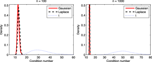
Figure 1: Distributions of the condition number of $\widetilde{p}{}^{-1}\mathbf{X}\mathbf{X}^{T}$ in different scenarios of distributions of $\mathbf{X}$ with $\widetilde{p}=3n$ and $n=100$ and $1000$, based on 100 simulations.

4 Numerical examples

In this section we provide two simulation examples to illustrate the theoretical results in Section 2, obtained through probabilistic arguments. The first simulation example examines the concentration property for large random design matrix. Let $\mathbf{X}$ be an $n\times\widetilde{p}$ random design matrix with $\widetilde{p}=cn$ for some constant $c>1$. We set $n=100$ and $1000$, and $c=3$. We considered three scenarios of distributions: (1) each entry of $\mathbf{X}$ is sampled independently from $N(0,1)$, (2) each entry of $\mathbf{X}$ is sampled independently from the Laplace distribution with mean 0 and variance 1, and (3) each row of $\mathbf{X}$ is sampled independently from the multivariate $t$-distribution with 10 degrees of freedom and then rescaled to have unit variances. In view of Definition 1, the concentration property of $\mathbf{X}$ is characterized by the distribution of the condition number of $\widetilde{p}{}^{-1}\mathbf{X}\mathbf{X}^{T}$. In each case, 100 Monte Carlo simulations were used to obtain the distribution of such condition number. Figure 1 depicts these distributions in different scenarios. We see that in scenarios 1 and 2, the condition number concentrates in the range of relatively small numbers, indicating the associated concentration property as shown in Theorem 1. In scenario 3 with multivariate $t$-distribution, one still observes the concentration phenomenon. However, since this distribution is relatively more heavy-tailed, we see that the distribution of the condition number becomes more spread out and shifts toward the range of large numbers.

The second simulation example investigates the robust spark bound for large $n\times p$ random design matrix $\mathbf{X}$. We adopted the same three scenarios of distributions as in the first simulation example, except that $n=100$, and $p=1000$ and $5000$. In light of Theorem 2, we sampled randomly 1000 $n\times k$ submatrices of $n^{-1/2}\mathbf{X}$ each with $k=\lceil 2n/(\log p)\rceil$ columns and calculated the minimum of those 1000 smallest singular values. Similarly, in each case 100 Monte Carlo simulations were used to obtain the distribution of such minimum singular value which is tied to the

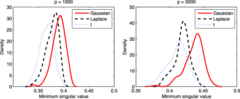
Figure 2: Distributions of the minimum singular value over 1000 submatrices of $n^{-1/2}\mathbf{X}$ each with $\lceil 2n/(\log p)\rceil$ columns, in different scenarios of distributions of $\mathbf{X}$ with $n=100$, and $p=1000$ and $5000$, based on 100 simulations.

robust spark bound of $\mathbf{X}$. These distributions are shown in Figure 2. In particular, we see that the distribution of the minimum singular value concentrates clearly away from zero in each of the three scenarios of distributions. These numerical results indicate that the robust spark of random design matrix can indeed be at least of order $O\{n/(\log p)\}$, as shown in Theorem 2.

5 Discussions

We have investigated the impacts of high dimensionality in finite samples from two different perspectives: a probabilistic one and a nonprobabilistic one. An interesting concentration phenomenon for large random design matrix has been revealed, as shown previously in Hall, Marron and Neeman (2005). We have shown that the concentration property, which is important in characterizing the sure screening property of the SIS, holds for a wide class of elliptical distributions, as conjectured by Fan and Lv (2008). We have also established a lower bound on the robust spark which is important in ensuring model identifiability and stable estimation. The high-dimensional geometric view of finite samples has lead to general bounds on dimensionality with distance constraint on sparse models, using nonprobabilistic arguments.

Both probabilistic and nonprobabilistic views provide understandings on how the dimensionality interacts with the sample size for large-scale data sets. Characterizing the limit of the dimensionality with respect to the sample size is key to the success of high-dimensional inference goals such as prediction and variable selection. We have focused on the family of elliptical distributions. It would be interesting to consider a more general class of distributions for future research.

Appendix A Proofs of main results

For notational simplicity, we use $C$ to denote a generic positive constant, whose value may change from line to line.

A.1 Proof of Lemma 1

By Theorem 5.2 in Ledoux (2001), we know that Condition 1 entails the logarithmic Sobolev inequality (4) when $\widetilde{\mu}_{q}=\mu_{p}$. It remains to prove the logarithmic Sobolev inequality for any marginal distribution of $\mu_{p}$. Let $1\leq q<p$ and $\widetilde{\mu}_{q}$ be a $q$-variate marginal distribution of $\mu_{p}$. By the spherical symmetry of $\mu_{p}$, without loss of generality we can assume that $\widetilde{\mu}_{q}$ is concentrated on $\mathbb{R}^{q}=\{\mathbf{v}=(v_{1},\ldots,v_{p})^{T}\in\mathbb{R}^{p}\dvtx v_{q+1}=\cdots=v_{p}=0\}$. For any smooth function $\widetilde{f}$ on $\mathbb{R}^{q}$ with $E_{\widetilde{\mu}_{q}}\widetilde{f}{}^{2}=1$, define $f\dvtx\mathbb{R}^{p}\rightarrow\mathbb{R}$ by

$$f(v_{1},\ldots,v_{q},v_{q+1},\ldots,v_{p})=\widetilde{f}(v_{1},\ldots,v_{q}).$$ (11)

Clearly $f$ is a smooth function on $\mathbb{R}^{p}$ and

$$\nabla f(v_{1},\ldots,v_{q},v_{q+1},\ldots,v_{p})=\left[\matrix{\nabla\widetilde{f}(v_{1},\ldots,v_{q})\cr\mathbf{0}}\right],$$

which shows that

$$\bigl{\|}\nabla f(v_{1},\ldots,v_{q},v_{q+1},\ldots,v_{p})\bigr{\|}_{2}^{2}=\bigl{\|}\nabla\widetilde{f}(v_{1},\ldots,v_{q})\bigr{\|}_{2}^{2}.$$ (12)

In view of (11), it follows from Fubini’s theorem that

$$E_{\mu_{p}}f^{2}=E_{\widetilde{\mu}_{q}}\widetilde{f}{}^{2}=1.$$

Thus by (11), (12), and Fubini’s theorem, applying the logarithmic Sobolev inequality (4) for $\mu_{p}$ to the smooth function $f$ yields

$$E_{\widetilde{\mu}_{q}}\bigl{\{}\widetilde{f}{}^{2}\log\widetilde{f}{}^{2}\bigr{\}}=E_{\mu_{p}}\bigl{\{}f^{2}\log f^{2}\bigr{\}}\leq 2C_{2}E_{\mu_{p}}\|\nabla f\|_{2}^{2}=2C_{2}E_{\widetilde{\mu}_{q}}\|\nabla\widetilde{f}\|_{2}^{2},$$

which completes the proof.

A.2 Proof of Lemma 2

We first prove part (a). By Lemma 1, the distribution of $\mathbf{z}_{q}$ satisfies the logarithmic Sobolev inequality (4). Observe that by the triangle inequality, the Euclidean norm $\|\cdot\|_{2}$ is $1$-Lipschitz with respect to the metric induced by itself. Therefore, the classical Herbst argument applies to prove the concentration inequality (5) [see, e.g., Theorem 5.3 in Ledoux (2001)]. It remains to show part (b). Note that $EZ_{1}^{2}=1$. By the spherical symmetry of $\mu_{p}$, Hölder’s inequality, and the Cauchy–Schwarz inequality, we have

$$E\|\mathbf{z}_{q}\|_{2}\leq\sqrt{E\|\mathbf{z}_{q}\|_{2}^{2}}=\sqrt{qEZ_{1}^{2}}=\sqrt{q}$$

and

$$E\|\mathbf{z}_{q}\|_{2}\geq E\bigl{(}q^{-1/2}\|\mathbf{z}_{q}\|_{1}\bigr{)}=\sqrt{q}E|Z_{1}|.$$

This concludes the proof.

A.3 Proof of Lemma 3

We first make a simple observation. The standard Gaussian distributions are special cases of spherical distributions. Recall that the $q$-variate standard Gaussian distribution $\gamma_{q}$ has density function $\frac{1}{(2\pi)^{q/2}}e^{-\|\mathbf{v}\|_{2}^{2}/2}$, $\mathbf{v}\in\mathbb{R}^{q}$. Thus it is easy to check that $\gamma_{q}$ satisfies Condition 1 with $c_{2}=1$. Let $\mathbf{w}=(W_{1},\ldots,W_{q})^{T}\sim N(\mathbf{0},I_{q})$. Then it follows immediately from Lemma 2 that for any $r\in(0,\infty)$,

$$P\bigl{(}\bigl{|}\|\mathbf{w}\|_{2}-E\|\mathbf{w}\|_{2}\bigr{|}>r\bigr{)}\leq 2e^{-r^{2}/2}.$$ (13)

Note that

$$E|W_{1}|=2\int_{0}^{\infty}u\frac{1}{\sqrt{2\pi}}e^{-u^{2}/2}\,du=\sqrt{\frac{2}{\pi}}\int_{0}^{\infty}e^{-u^{2}/2}\,d\biggl{(}\frac{u^{2}}{2}\biggr{)}=\sqrt{\frac{2}{\pi}}.$$ (14)

By (6), (13), and (14), we have for any $r_{1}\in(0,\sqrt{\frac{2}{\pi}})$,

$$P\biggl{(}q^{-1/2}\|\mathbf{w}\|_{2}>1+r_{1}\mbox{ or }q^{-1/2}\|\mathbf{w}\|_{2}<\sqrt{\frac{2}{\pi}}-r_{1}\biggr{)} \leq 2e^{-qr_{1}^{2}/2}$$

$$\leq 2e^{-nr_{1}^{2}/2}$$

since $q\geq n$.

Now we get back to $\mathbf{z}_{q}$. It follows from (5) and (6) in Lemma 2 and Condition 2 that for any $r_{2}\in(0,c_{3})$,

$$P\bigl{(}q^{-1/2}\|\mathbf{z}_{q}\|_{2}>1+r_{2}\mbox{ or }q^{-1/2}\|\mathbf{z}_{q}\|_{2}<c_{3}-r_{2}\bigr{)} \leq 2e^{-C_{2}^{-1}qr_{2}^{2}/2}$$

$$\leq 2e^{-C_{2}^{-1}nr_{2}^{2}/2}$$

since $q\geq n$. Let

$$c_{4}=\frac{c_{3}-r_{2}}{1+r_{1}}\quad\mbox{and}\quad c_{5}=\frac{1+r_{2}}{\sqrt{{2}/{\pi}}-r_{1}}.$$

Then combining (A.3) and (A.3) along with Bonferroni’s inequality yields

$$P\biggl{(}\frac{\|\mathbf{z}_{q}\|_{2}}{\|\mathbf{w}\|_{2}}<c_{4}\mbox{ or }\frac{\|\mathbf{z}_{q}\|_{2}}{\|\mathbf{w}\|_{2}}>c_{5}\biggr{)} \leq 2e^{-nr_{1}^{2}/2}+2e^{-C_{2}^{-1}nr_{2}^{2}/2}$$

$$\leq 4e^{-C_{3}n},$$

where $C_{3}=\min(r_{1}^{2}/2,C_{2}^{-1}r_{2}^{2}/2)$. This completes the proof.

A.4 Proof of Theorem 1

In Section A.7, Fan and Lv (2008) proved that Gaussian distributions satisfy the concentration property (2), that is, for $\mathbf{Z}\sim N(\mathbf{0},I_{n}\otimes I_{p})=N(\mathbf{0},I_{n\times p})$. We now consider the general situation where $n$ rows of the $n\times p$ random matrix $\mathbf{Z}=(\mathbf{z}_{1},\ldots,\mathbf{z}_{n})^{T}$ are i.i.d. copies from the spherical distribution $\mu_{p}$. Fix an arbitrary $n\times\widetilde{p}$ submatrix $\widetilde{\mathbf{Z}}$ of $\mathbf{Z}$ with $cn<\widetilde{p}\leq p$, where $c\in(1,\infty)$. We aim to prove deviation inequality in (2) with different constants $c_{1}\in(1,\infty)$ and $C_{1}\in(0,\infty)$.

By the spherical symmetry, without loss of generality we can assume that $\widetilde{\mathbf{Z}}$ consists of the first $\widetilde{p}$ columns of $\mathbf{Z}$. Let

$$\widetilde{\mathbf{z}}=(Z_{1},\ldots,Z_{\widetilde{p}})^{T}\quad\mbox{and}\quad\widetilde{\mathbf{Z}}=(\widetilde{\mathbf{z}}_{1},\ldots,\widetilde{\mathbf{z}}_{n})^{T}.$$

Clearly, $\widetilde{\mathbf{z}}_{1},\ldots,\widetilde{\mathbf{z}}_{n}$ are $n$ i.i.d. copies of $\widetilde{\mathbf{z}}$. Take an $n\times\widetilde{p}$ random matrix

$$\mathbf{W}=(\mathbf{w}_{1},\ldots,\mathbf{w}_{n})^{T}\sim N(\mathbf{0},I_{n}\otimes I_{\widetilde{p}}),$$

which is independent of $\widetilde{\mathbf{Z}}$. Then for each $i=1,\ldots,n$, $\mathbf{w}_{i}$ has the $\widetilde{p}$-variate standard Gaussian distribution. It is well known that $\mathbf{w}_{i}/\|\mathbf{w}_{i}\|_{2}$ has the Haar distribution on the unit sphere $S^{\widetilde{p}-1}$ in $\widetilde{p}$-dimensional Euclidean space $\mathbb{R}^{\widetilde{p}}$, that is, the uniform distribution on $S^{\widetilde{p}-1}$.

Since the distribution of $\widetilde{\mathbf{z}}$ is a marginal distribution of $\mu_{p}$, the spherical symmetry of $\mu_{p}$ entails that of the distribution of $\widetilde{\mathbf{z}}$. It follows easily from the assumption of $P(\mathbf{z}=\mathbf{0})=0$ that $P(\widetilde{\mathbf{z}}=\mathbf{0})=0$. Thus by Theorem 1.5.6 in Muirhead (1982), $\widetilde{\mathbf{z}}/\|\widetilde{\mathbf{z}}\|_{2}$ is uniformly distributed on $S^{\widetilde{p}-1}$ and is independent of $\|\widetilde{\mathbf{z}}\|_{2}$. This along with the above fact shows that for each $i=1,\ldots,n$,

$$\widetilde{\mathbf{z}}_{i}\stackrel{{\scriptstyle\mathrm{(d)}}}{{=}}\|\widetilde{\mathbf{z}}_{i}\|_{2}\biggl{(}\frac{\mathbf{w}_{i}}{\|\mathbf{w}_{i}\|_{2}}\biggr{)}=\biggl{(}\frac{\|\widetilde{\mathbf{z}}_{i}\|_{2}}{\|\mathbf{w}_{i}\|_{2}}\biggr{)}\mathbf{w}_{i},$$ (17)

where we use the symbol $\stackrel{{\scriptstyle\mathrm{(d)}}}{{=}}$ to denote being identical in distribution. Hereafter, for notational simplicity we do not distinguish $\widetilde{\mathbf{z}}_{i}$ and $(\frac{\|\widetilde{\mathbf{z}}_{i}\|_{2}}{\|\mathbf{w}_{i}\|_{2}})\mathbf{w}_{i}$.

Define the $n\times n$ diagonal matrix

$$\mathbf{Q}=\operatorname{diag}\biggl{\{}\frac{\|\widetilde{\mathbf{z}}_{1}\|_{2}}{\|\mathbf{w}_{1}\|_{2}},\ldots,\frac{\|\widetilde{\mathbf{z}}_{n}\|_{2}}{\|\mathbf{w}_{n}\|_{2}}\biggr{\}}.$$

Then we have

$$\widetilde{p}{}^{-1}\widetilde{\mathbf{Z}}\widetilde{\mathbf{Z}}{}^{T}=\mathbf{Q}\bigl{(}\widetilde{p}{}^{-1}\mathbf{W}\mathbf{W}^{T}\bigr{)}\mathbf{Q},$$

which entails

$$\min_{i=1}^{n}\frac{\|\widetilde{\mathbf{z}}_{i}\|_{2}^{2}}{\|\mathbf{w}_{i}\|_{2}^{2}}\lambda_{\mathrm{min}}\bigl{(}\widetilde{p}{}^{-1}\mathbf{W}\mathbf{W}^{T}\bigr{)}I_{n} \leq \min_{i=1}^{n}\frac{\|\widetilde{\mathbf{z}}_{i}\|_{2}^{2}}{\|\mathbf{w}_{i}\|_{2}^{2}}\bigl{(}\widetilde{p}{}^{-1}\mathbf{W}\mathbf{W}^{T}\bigr{)}\leq\mathbf{Q}\bigl{(}\widetilde{p}{}^{-1}\mathbf{W}\mathbf{W}^{T}\bigr{)}\mathbf{Q}$$

$$= \widetilde{p}{}^{-1}\widetilde{\mathbf{Z}}\widetilde{\mathbf{Z}}{}^{T}\leq\max_{i=1}^{n}\frac{\|\widetilde{\mathbf{z}}_{i}\|_{2}^{2}}{\|\mathbf{w}_{i}\|_{2}^{2}}\bigl{(}\widetilde{p}{}^{-1}\mathbf{W}\mathbf{W}^{T}\bigr{)}$$

$$\leq \max_{i=1}^{n}\frac{\|\widetilde{\mathbf{z}}_{i}\|_{2}^{2}}{\|\mathbf{w}_{i}\|_{2}^{2}}\lambda_{\mathrm{max}}\bigl{(}\widetilde{p}{}^{-1}\mathbf{W}\mathbf{W}^{T}\bigr{)}I_{n}.$$

This shows that

$$\lambda_{\mathrm{min}}\bigl{(}\widetilde{p}{}^{-1}\widetilde{\mathbf{Z}}\widetilde{\mathbf{Z}}{}^{T}\bigr{)}\geq\min_{i=1}^{n}\frac{\|\widetilde{\mathbf{z}}_{i}\|_{2}^{2}}{\|\mathbf{w}_{i}\|_{2}^{2}}\lambda_{\mathrm{min}}\bigl{(}\widetilde{p}{}^{-1}\mathbf{W}\mathbf{W}^{T}\bigr{)}$$ (18)

and

$$\lambda_{\mathrm{max}}\bigl{(}\widetilde{p}{}^{-1}\widetilde{\mathbf{Z}}\widetilde{\mathbf{Z}}{}^{T}\bigr{)}\leq\max_{i=1}^{n}\frac{\|\widetilde{\mathbf{z}}_{i}\|_{2}^{2}}{\|\mathbf{w}_{i}\|_{2}^{2}}\lambda_{\mathrm{max}}\bigl{(}\widetilde{p}{}^{-1}\mathbf{W}\mathbf{W}^{T}\bigr{)}.$$ (19)

As mentioned before, we have for some $c_{1}\in(1,\infty)$ and $C_{1}\in(0,\infty)$,

$$P\bigl{(}\lambda_{\mathrm{max}}\bigl{(}\widetilde{p}{}^{-1}\mathbf{W}\mathbf{W}^{T}\bigr{)}>c_{1}\mbox{ or }\lambda_{\mathrm{min}}\bigl{(}\widetilde{p}{}^{-1}\mathbf{W}\mathbf{W}^{T}\bigr{)}<1/c_{1}\bigr{)}\leq e^{-C_{1}n}.$$ (20)

Note that $\widetilde{p}>n$. Thus by (7) in Lemma 3, an application of Bonferroni’s inequality gives

$$P\biggl{(}\min_{i=1}^{n}\frac{\|\widetilde{\mathbf{z}}_{i}\|_{2}^{2}}{\|\mathbf{w}_{i}\|_{2}^{2}}<c_{4}\mbox{ or }\max_{i=1}^{n}\frac{\|\widetilde{\mathbf{z}}_{i}\|_{2}^{2}}{\|\mathbf{w}_{i}\|_{2}^{2}}>c_{5}\biggr{)}\leq 4ne^{-C_{3}n},$$ (21)

where $c_{4}\in(0,1)$, $c_{5}\in(1,\infty)$, and $C_{3}\in(0,\infty)$. Therefore by Bonferroni’s inequality, combining (20) and (21) proves the deviation inequality in (2) by appropriately changing the constants $c_{1}\in(1,\infty)$ and $C_{1}\in(0,\infty)$. This concludes the proof.

A.5 Proof of Theorem 2

Using the similar arguments as in the proof of Theorem 1, we can prove that there exist some universal positive constants $c_{6},C$ such that the deviation probability bound

$$P\bigl{\{}\lambda_{\min}\bigl{(}n^{-1}\widetilde{\mathbf{Z}}{}^{T}\widetilde{\mathbf{Z}}\bigr{)}<c_{6}\bigr{\}}\leq\exp(-Cn)$$ (22)

holds for each $n\times\widetilde{p}$ submatrix $\widetilde{\mathbf{Z}}$ of $\mathbf{Z}$ with $\widetilde{p}=c_{7}n$ and $c_{7}<1$ some positive constant. This is because Lemmas 1–2 are free of the dimension $q$ of the marginal distribution, and Lemma 3 still holds with the choice of $q=\widetilde{p}$. We should also note that the deviation probability bound (22) holds when $\widetilde{\mathbf{Z}}\sim N(\mathbf{0},I_{n}\otimes I_{\widetilde{p}})$, which is entailed by the concentration property (2) proved in Fan and Lv (2008) for Gaussian distributions.

For each set $\alpha\subset\{1,\ldots,p\}$ with $|\alpha|=\widetilde{p}$, denote by $\bolds{\Sigma}_{\alpha,\alpha}$ the principal submatrix of $\bolds{\Sigma}$ corresponding to variables in $\alpha$, and $\mathbf{X}_{\alpha}$ a submatrix of the design matrix $\mathbf{X}$ consisting of columns with indices in $\alpha$. It follows easily from the representation of elliptical distributions that $\widetilde{\mathbf{X}}_{\alpha}=\mathbf{X}_{\alpha}\bolds{\Sigma}_{\alpha,\alpha}^{-1/2}$ has the same distribution as $\mathbf{Z}_{\alpha}$. Since $\lambda_{\min}(\bolds{\Sigma})$ is bounded from below by some positive constant, we have

$$\lambda_{\min}\bigl{(}n^{-1}\mathbf{X}_{\alpha}^{T}\mathbf{X}_{\alpha}\bigr{)}\geq\lambda_{\min}\bigl{(}n^{-1}\widetilde{\mathbf{X}}_{\alpha}^{T}\widetilde{\mathbf{X}}_{\alpha}\bigr{)}\lambda_{\min}(\bolds{\Sigma}_{\alpha,\alpha})\geq C\lambda_{\min}\bigl{(}n^{-1}\widetilde{\mathbf{X}}_{\alpha}^{T}\widetilde{\mathbf{X}}_{\alpha}\bigr{)},$$

where $C$ is some positive constant. Therefore, combining the above results yields

$$P\bigl{\{}\lambda_{\min}\bigl{(}n^{-1}\mathbf{X}_{\alpha}^{T}\mathbf{X}_{\alpha}\bigr{)}<c_{6}\bigr{\}}\leq\exp(-Cn)$$ (23)

with a possibly different positive constant $c_{6}$. Note that the positive constants involved are universal ones. We choose a positive integer $K=2^{-1}Cn/\break(\log p)\leq\widetilde{p}$. Then an application of the Bonferroni inequality together with (23) gives

$$P\Bigl{\{}\min_{|\alpha|=K}\lambda_{\min}\bigl{(}n^{-1}\mathbf{X}_{\alpha}^{T}\mathbf{X}_{\alpha}\bigr{)}<c_{6}\Bigr{\}}\leq\sum_{|\alpha|=K}\exp(-Cn)\leq p^{K}\exp(-Cn)\rightarrow 0$$

as $n\rightarrow\infty$. This shows that with asymptotic probability one, the robust spark $\kappa_{c}\geq K$ for any $c\leq c_{6}$, which completes the proof.

A.6 Proof of Theorem 3

For the maximum chordal distance $d_{m}$, by noting that $x_{i}=\sin^{2}\theta_{i}$, we have a simple representation of the neighborhood $B_{\delta,d_{m}}=\{(x_{1},\ldots,x_{s})\in[0,1]^{s}\dvtx\max_{i=1}^{s}x_{i}\leq\delta^{2}\}$ for $\delta\in(0,1/2)$. We need to calculate its volume under the probability measure $\nu$ given in (43). In light of (43), a change of variable $y_{i}=\delta^{-2}x_{i}$ gives

$$\quad d\nu=\delta^{s(n-s)}K_{n,s}f(y_{1},\ldots,y_{s})\prod_{1\leq i<j\leq s}|y_{i}-y_{j}|\prod_{i=1}^{s}y_{i}^{\alpha-1}\,dy_{1}\cdots dy_{s},$$ (24)

where $f(y_{1},\ldots,y_{s})=\prod_{i=1}^{s}(1-\delta^{2}y_{i})^{-1/2}$ over $[0,1]^{s}$. Observe that without the term $f$ in (24), $\nu(B_{\delta,d_{m}})$ would become Selberg’s integral which is a generalization of the beta integral [Mehta (2004)]. We will evaluate this integral by sandwiching the function $f$ between two functions of the same form. Since the function $(1-\delta^{2}y)^{-1/2}$ is increasing and convex on $[0,1]$, it follows that $1+c_{1}y\leq(1-\delta^{2}y)^{-1/2}\leq 1+c_{2}y$, where $c_{1}=\delta^{2}/2$ and $c_{2}=\delta^{2}(1-\delta^{2})^{-3/2}/2$. This shows that

$$\prod_{i=1}^{s}(1+c_{1}y_{i})\leq f(y_{1},\ldots,y_{s})\leq\prod_{i=1}^{s}(1+c_{2}y_{i}).$$

Thus, we obtain a useful representation of the volume of the neighborhood

$$\nu(B_{\delta,d_{m}})=\delta^{s(n-s)}K_{n,s}I(c),$$ (25)

where $I(c)$ with some $c\in[c_{1},c_{2}]$ is an integral given in the following lemma.

Lemma 4.

For each $c>0$, we have

$$I(c) \equiv \int_{[0,1]^{s}}\prod_{i=1}^{s}(1+cy_{i})\prod_{1\leq i<j\leq s}|y_{i}-y_{j}|\prod_{i=1}^{s}y_{i}^{\alpha-1}\,dy_{1}\cdots dy_{s}$$

$$= 2^{s}\pi^{-s/2}\sum_{m=0}^{s}\pmatrix{s\cr m}c^{m}\prod_{i=s-m}^{s-1}\frac{\alpha+2^{-1}i}{\alpha+2^{-1}(s+i+1)}$$

$${}\times\prod_{i=0}^{s-1}\frac{\Gamma(\alpha+2^{-1}i)\Gamma(1+2^{-1}(i+1))\Gamma(1+2^{-1}i)}{\Gamma(\alpha+2^{-1}(s+i+1))},$$

where the factor containing $m$ equals $1$ when $m=0$.

Observe that the integrand in (4) is symmetric in $y_{1},\ldots,y_{s}$. Thus, an expansion of $\prod_{i=1}^{s}(1+cy_{i})$ gives

$$\int_{[0,1]^{s}}\prod_{i=1}^{s}(1+cy_{i})\prod_{1\leq i<j\leq s}|y_{i}-y_{j}|\prod_{i=1}^{s}y_{i}^{\alpha-1}\,dy_{1}\cdots dy_{s}$$

$$\qquad=\sum_{m=0}^{s}\pmatrix{s\cr m}c^{m}\int_{[0,1]^{s}}\prod_{i=1}^{m}y_{i}\prod_{1\leq i<j\leq s}|y_{i}-y_{j}|\prod_{i=1}^{s}y_{i}^{\alpha-1}\,dy_{1}\cdots dy_{s},$$

where $\prod_{i=1}^{m}y_{i}=1$ when $m=0$. The above integrals are exactly Aomoto’s extension of Selberg’s integral [Mehta (2004)] and can be calculated as

$$\int_{[0,1]^{s}}\prod_{i=1}^{m}y_{i}\prod_{1\leq i<j\leq s}|y_{i}-y_{j}|\prod_{i=1}^{s}y_{i}^{\alpha-1}\,dy_{1}\cdots dy_{s}$$

$$\qquad=2^{s}\pi^{-s/2}\prod_{i=s-m}^{s-1}\frac{\alpha+2^{-1}i}{\alpha+2^{-1}(s+i+1)}$$

$$\qquad\quad{}\times\prod_{i=0}^{s-1}\frac{\Gamma(\alpha+2^{-1}i)\Gamma(1+2^{-1}(i+1))\Gamma(1+2^{-1}i)}{\Gamma(\alpha+2^{-1}(s+i+1))},$$

where the factor containing $m$ equals $1$ when $m=0$. This completes the proof of Lemma 4.

Let us continue with the proof of Theorem 3. By assumption, $s\sim\gamma n$ as $n\rightarrow\infty$, so $\delta^{s(n-s)}\pi^{-s/2}\sim\delta^{\gamma(1-\gamma)n^{2}}\pi^{-\gamma n/2}$. Applying Stirling’s formula for large factorials gives $s!\sim(2\pi\gamma n)^{1/2}(\gamma/e)^{\gamma n}n^{\gamma n}$. Thus by omitting $O(n)$ and smaller order terms,

$$\log\bigl{[}\delta^{s(n-s)}\pi^{-s/2}/s!\bigr{]}\sim(\log\delta)\gamma(1-\gamma)n^{2}-\gamma n\log n.$$ (27)

Using Stirling’s formula for the Gamma function $\Gamma(t+1)\sim(2\pi t)^{1/2}(t/e)^{t}$ as $t\rightarrow\infty$ and noting that $A_{j}=2\pi^{j/2}/\Gamma(j/2)$ and $\alpha=(n-2s+1)/2$, we derive

$$\prod_{i=0}^{s-1}\frac{A_{n-s-i}}{A_{n-i}}\prod_{i=0}^{s-1}\frac{\Gamma(\alpha+2^{-1}i)}{\Gamma(\alpha+2^{-1}(s+i+1))}$$

$$\qquad\sim\pi^{-s^{2}/2}(2e)^{s/2}(n-s-1)^{(n-s-1)/2}(n-1)^{-(n-1)/2},$$

which entails that

$$\log\Biggl{\{}\prod_{i=0}^{s-1}\frac{A_{n-s-i}}{A_{n-i}}\prod_{i=0}^{s-1}\frac{\Gamma(\alpha+2^{-1}i)}{\Gamma(\alpha+2^{-1}(s+i+1))}\Biggr{\}}$$

(28)

$$\qquad\sim-(\log\pi)\gamma^{2}n^{2}/2-\gamma n(\log n)/2.$$

Similarly, it follows from the identities $\Gamma(t+1)=t\Gamma(t)$ and $\Gamma(1)=1$ that

$$2^{-s}\prod_{i=0}^{s-1}A_{s-i}^{2}\prod_{i=0}^{s-1}\Gamma\bigl{(}1+2^{-1}(i+1)\bigr{)}\Gamma\bigl{(}1+2^{-1}i\bigr{)}=s!\pi^{s(s+1)/2}/\Gamma(s/2).$$

This shows that

$$\log\Biggl{\{}2^{-s}\prod_{i=0}^{s-1}A_{s-i}^{2}\prod_{i=0}^{s-1}\Gamma\bigl{(}1+2^{-1}(i+1)\bigr{)}\Gamma\bigl{(}1+2^{-1}i\bigr{)}\Biggr{\}}$$

(29)

$$\qquad\sim(\log\pi)\gamma^{2}n^{2}/2+\gamma n(\log n)/2.$$

It remains to consider the last term. Note that

$$\prod_{i=s-m}^{s-1}\frac{\alpha+2^{-1}i}{\alpha+2^{-1}(s+i+1)}$$

$$\qquad=\frac{(n-s)!}{(n+1)!}\frac{(n-m+1)!}{(n-m-s)!}$$

$$\qquad\sim\biggl{(}\frac{n-m+1}{n+1}\biggr{)}^{s+1}\biggl{(}\frac{n-s}{n+1}\biggr{)}^{n-s+1/2}\biggl{(}\frac{n-m+1}{n-m-s}\biggr{)}^{n-m-s+1/2}$$

$$\qquad\sim e^{O(n)},$$

which entails that

$$\log\Biggl{\{}\sum_{m=0}^{s}\pmatrix{s\cr m}c^{m}\prod_{i=s-m}^{s-1}\frac{\alpha+2^{-1}i}{\alpha+2^{-1}(s+i+1)}\Biggr{\}} \sim \log\bigl{[}e^{O(n)}(1+c)^{s}\bigr{]}$$

$$= O(n).$$

Thus combining (25) and (27)–(A.6) yields

$$\log\bigl{(}\nu(B_{\delta,d_{m}})\bigr{)}\sim(\log\delta)\gamma(1-\gamma)n^{2}-\gamma n\log n+O(n).$$ (31)

Since all the subspaces in $\mathcal{A}_{s}$ have maximum chordal distance at least $2\delta$, it holds that ${p\choose s}=|\mathcal{A}_{s}|\leq 1/\nu(B_{\delta,d_{m}})$. Hence by (31),

$$\log\pmatrix{p\cr s}\lesssim\bigl{(}\log\delta^{-1}\bigr{)}\gamma(1-\gamma)n^{2}+\gamma n\log n+O(n),$$

where $\lesssim$ denotes asymptotic dominance. It is easy to derive $\log{p\choose s}\gtrsim\gamma n\log p-\gamma n\log n$. These two results lead to the claimed bound on $\log p$, which concludes the proof.

A.7 Proof of Theorem 4

Let us fix an arbitrary subset $\{\mathbf{x}_{j_{1}},\ldots,\mathbf{x}_{j_{s}}\}$ and denote by $\mathcal{A}_{s}^{p-s}$ the set of $s$-subspaces spanned by $s$ of the remaining $p-s$ $\mathbf{x}_{j}$’s. By assumption, $\mathcal{A}_{s}^{p-s}$ lies in a neighborhood in the Grassmann manifold $G_{n,s}$ that is characterized by the set $R_{\delta_{1}}=\{(x_{1},\ldots,x_{s})\in[0,1]^{s}\dvtx\min_{i=1}^{s}x_{i}\geq\delta_{1}^{2}\}$, since $x_{i}=\sin^{2}\theta_{i}$. In view of (43), a change of variable $y_{i}=(1-\delta_{1}^{2})^{-1}(1-x_{i})$ gives

$$d\nu = \bigl{(}1-\delta_{1}^{2}\bigr{)}^{s^{2}/2}K_{n,s}f_{1}(y_{1},\ldots,y_{s})$$

$${}\times\prod_{1\leq i<j\leq s}|y_{i}-y_{j}|\prod_{i=1}^{s}y_{i}^{-1/2}\,dy_{1}\cdots dy_{s},$$

where $f_{1}(y_{1},\ldots,y_{s})=\prod_{i=1}^{s}[1-(1-\delta_{1}^{2})y_{i}]^{\alpha-1}$ over $[0,1]^{s}$. Clearly $[1-(1-\delta_{1}^{2})y_{i}]^{\alpha-1}\geq(1-y_{i})^{\alpha-1}$ for $\alpha\geq 1$, which together with (43) and (A.7) entails that $(1-\delta_{1}^{2})^{s^{2}/2}$ is a lower bound on the integral $\nu(R_{\delta_{1}})$. However, we need an upper bound on it. The idea is to bound the function $f_{1}$ by an exponential function.

We are more interested in the asymptotic behavior of $\nu(R_{\delta_{1}})$ when $\delta_{1}$ is near zero. Using the inequality $\log(1+t)\leq t$, we derive

$$1-\bigl{(}1-\delta_{1}^{2}\bigr{)}y=\bigl{(}1-\delta_{1}^{2}\bigr{)}\bigl{[}1+\bigl{(}1-\delta_{1}^{2}\bigr{)}^{-1}\delta_{1}^{2}-y\bigr{]}\leq\bigl{(}1-\delta_{1}^{2}\bigr{)}e^{(1-\delta_{1}^{2})^{-1}\delta_{1}^{2}}e^{-y}.$$

This leads to

$$f_{1}(y_{1},\ldots,y_{s})\leq\bigl{[}\bigl{(}1-\delta_{1}^{2}\bigr{)}e^{(1-\delta_{1}^{2})^{-1}\delta_{1}^{2}}\bigr{]}^{s(\alpha-1)}\prod_{i=1}^{s}e^{-(\alpha-1)y_{i}}.$$

Thus we have

$$\nu(R_{\delta_{1}})\leq\bigl{(}1-\delta_{1}^{2}\bigr{)}^{2^{-1}s^{2}+s(\alpha-1)}e^{(1-\delta_{1}^{2})^{-1}\delta_{1}^{2}s(\alpha-1)}K_{n,s}B_{\alpha},$$ (33)

where $B_{\alpha}=\int_{[0,1]^{s}}\prod_{1\leq i<j\leq s}|y_{i}-y_{j}|\prod_{i=1}^{s}y_{i}^{-1/2}e^{-(\alpha-1)y_{i}}\,dy_{1}\cdots dy_{s}$. Since $\alpha-1=(n-2s-1)/2\rightarrow\infty$ as $n\rightarrow\infty$, a change of variable $z_{i}=(\alpha-1)y_{i}$ gives

$$B_{\alpha} = (\alpha-1)^{-s^{2}/2}\int_{[0,\alpha-1]^{s}}\prod_{1\leq i<j\leq s}|z_{i}-z_{j}|\prod_{i=1}^{s}z_{i}^{-1/2}e^{-z_{i}}\,dz_{1}\cdots dz_{s}$$

$$\leq (\alpha-1)^{-s^{2}/2}\int_{[0,\infty)^{s}}\prod_{1\leq i<j\leq s}|z_{i}-z_{j}|\prod_{i=1}^{s}z_{i}^{-1/2}e^{-z_{i}}\,dz_{1}\cdots dz_{s}.$$

Note that the last integral is a Selberg type integral related to the Laguerre polynomials [Mehta (2004)], which can be calculated exactly. This along with the identities $\Gamma(t+1)=t\Gamma(t)$ and $\Gamma(3/2)=\pi^{1/2}/2$ yields

$$B_{\alpha}\lesssim(\alpha-1)^{-s^{2}/2}s!\pi^{-s/2}\prod_{i=1}^{s}\Gamma^{2}(i/2).$$

By assumption, $s\sim\gamma n$ as $n\rightarrow\infty$. It is easy to show that

$$\log\bigl{[}\bigl{(}1-\delta_{1}^{2}\bigr{)}^{2^{-1}s^{2}+s(\alpha-1)}e^{(1-\delta_{1}^{2})^{-1}\delta_{1}^{2}s(\alpha-1)}\bigr{]}\sim-c_{\delta_{1}}\gamma n^{2}+O(n),$$ (34)

where $c_{\delta_{1}}=2^{-1}[\log(1-\delta_{1}^{2})^{-1}](1-\gamma)-2^{-1}(1-\delta_{1}^{2})^{-1}\delta_{1}^{2}(1-2\gamma)$. It remains to consider the term $K_{n,s}B_{\alpha}$. By (42), we have

$$2^{-s}\pi^{-s/2}\widetilde{K}_{n,s}\prod_{i=1}^{s}\Gamma^{2}(i/2)$$

$$\qquad=\prod_{i=0}^{s-1}\frac{\Gamma((n-i)/2)}{\Gamma((n-s-i)/2)}$$

$$\qquad\sim\prod_{i=0}^{s-1}\biggl{(}\frac{n-i-2}{n-s-i-2}\biggr{)}^{(n-s-i-1)/2}\biggl{[}\frac{(n-2)!}{(n-s-2)!}\biggr{]}^{s/2}(2e)^{-s^{2}/2},$$

where we used Stirling’s formula for the Gamma function in the last step. It follows from $s\sim\gamma n$ that

$$\prod_{i=0}^{s-1}\biggl{(}\frac{n-i-2}{n-s-i-2}\biggr{)}^{(n-s-i-1)/2}\lesssim\biggl{(}\frac{1-\gamma}{1-2\gamma}\biggr{)}^{\gamma(1-\gamma)n^{2}/2},$$

and an application of Stirling’s formula for large factorials gives

$$\biggl{[}\frac{(n-2)!}{(n-s-2)!}\biggr{]}^{s/2}(2e)^{-s^{2}/2} \sim \biggl{(}\frac{n-2}{n-s-2}\biggr{)}^{s(n-s-3/2)/2}\bigl{[}(n-2)/\bigl{(}2e^{2}\bigr{)}\bigr{]}^{s^{2}/2}$$

$$\lesssim (1-\gamma)^{-\gamma(1-\gamma)n^{2}/2}\bigl{[}n/\bigl{(}2e^{2}\bigr{)}\bigr{]}^{\gamma^{2}n^{2}/2}.$$

Note that $(\alpha-1)^{-s^{2}/2}\sim[(1-2\gamma)n/2]^{-\gamma^{2}n^{2}/2}$. Combining these results together yields

$$\log(K_{n,s}B_{\alpha}) = \log\Biggl{[}(\alpha-1)^{-s^{2}/2}2^{-s}\pi^{-s/2}\widetilde{K}_{n,s}\prod_{i=1}^{s}\Gamma^{2}(i/2)\Biggr{]}$$

$$\lesssim -\bigl{[}2\gamma+\log(1-2\gamma)\bigr{]}\gamma n^{2}/2.$$

It follows from (33)–(A.7) that

$$\log\bigl{(}\nu(R_{\delta_{1}})\bigr{)}\lesssim-c_{\delta_{1}}\gamma n^{2}-\bigl{[}2\gamma+\log(1-2\gamma)\bigr{]}\gamma n^{2}/2+O(n).$$ (36)

Finally, we are ready to derive a bound on the dimensionality $p$. Since $\mathcal{A}_{s}^{p-s}$ lies in a neighborhood in $G_{n,s}$ characterized by the set $R_{\delta_{1}}$ and all the subspaces in $\mathcal{A}_{s}^{p-s}$ have maximum chordal distance at least $\delta$, it holds that ${p-s\choose s}=|\mathcal{A}_{s}^{p-s}|\leq\nu(R_{\delta_{1}})/\nu(B_{\delta,d_{m}})$. Aided by (31) and (36), a similar argument as in the proof of Theorem 3 gives the claimed bound on $\log(p-s)$. This completes the proof.

A.8 Proof of Theorem 5

To prove the conclusion, we use the terminology introduced in Section 3. Note that the $n$-vectors $\mathbf{x}_{j}$ and $\mathbf{y}$ can be viewed as elements of Grassmannian manifold $G_{n,1}$, which consists of all one-dimensional subspaces of $\mathbb{R}^{n}$. The absolute correlation between two $n$-vectors is given by $\cos\theta_{1}$, where $\theta_{1}\in[0,\pi/2]$ is the principal angle between the two corresponding one-dimensional subspaces. We use the parametrization with local coordinate $\theta_{1}$ at the one-dimensional subspace $L=\{t\mathbf{y}\dvtx t\in\mathbb{R}\}$ spanned by $\mathbf{y}$. Then the uniform distribution on the Grassmann manifold $G_{n,1}$ can be expressed in local coordinate $\theta_{1}$ and gives a probability measure $\nu$ in (43) with $s=1$ on $[0,1]$ through a change of variable $x_{1}=\sin^{2}\theta_{1}$, where $\prod_{1\leq i<j\leq s}|x_{i}-x_{j}|=1$ in this case. Consider the maximum chordal distance on $G_{n,1}$, which is defined as $\sin\theta_{1}$. For any $t>0$, denote by $B_{t,d_{m}}$ a ball of radius $t$ centered at $L$ in $G_{n,1}$ under the maximum chordal distance, that is, $B_{t,d_{m}}=\{x_{1}\in[0,1]\dvtx x_{1}=\sin^{2}\theta_{1}\leq t^{2}\}$ in local coordinate. We need to calculate the volumes of $B_{t_{1},d_{m}}$ with $t_{1}=2^{-1}\sin\cos^{-1}\delta=(1-\delta^{2})^{1/2}/2$ and $B_{t_{2},d_{m}}^{c}$, the complement of $B_{t_{2},d_{m}}$ with $t_{2}=\sin\cos^{-1}r=(1-r^{2})^{1/2}$, under the measure $\nu$.

In view of (43), we have

$$\nu(B_{t,d_{m}})=\nu\bigl{(}\bigl{[}0,t^{2}\bigr{]}\bigr{)}=K_{n,1}\int_{0}^{t^{2}}x_{1}^{(n-3)/2}(1-x_{1})^{-1/2}\,dx_{1},$$ (37)

where $K_{n,1}=\widetilde{K}_{n,1}/2=A_{1}^{2}A_{n-1}/(4A_{n})$ with $A_{j}=2\pi^{j/2}/\Gamma(j/2)$ the area of the unit sphere $S^{j-1}\subset\mathbb{R}^{j}$. It follows from Stirling’s formula for the Gamma function that

$$K_{n,1} = \pi^{-1/2}\Gamma(n/2)/\Gamma\bigl{(}(n-1)/2\bigr{)}$$

$$\sim \pi^{-1/2}\biggl{(}\frac{n-2}{2e}\biggr{)}^{1/2}\biggl{(}\frac{n-2}{n-3}\biggr{)}^{(n-2)/2}$$

$$\sim (2\pi)^{-1/2}n^{1/2}.$$

It remains to evaluate the integral in (37). Note that $(1-x_{1})^{-1/2}$ is bounded between $1$ and $\infty$ on $[0,t^{2}]$ for $t$ bounded away from $1$. Thus, we have

$$\quad\int_{0}^{t^{2}}x_{1}^{(n-3)/2}(1-x_{1})^{-1/2}\,dx_{1}>\int_{0}^{t^{2}}x_{1}^{(n-3)/2}\,dx_{1}=2(n-1)^{-1}t^{n-1},$$ (39)

where both sides have the same asymptotic order. Combining (37)–(39) yields $\nu(B_{t,d_{m}})>c_{n}t^{n-1}$ with $c_{n}\sim(2/\pi)^{1/2}n^{-1/2}$, and $\nu(B_{t,d_{m}})\sim\break(2/\pi)^{1/2}n^{-1/2}t^{n-1}$ for $t$ bounded away from $1$. Since all the $p-s$ noise predictors $\mathbf{x}_{j}$ have absolute correlations bounded by $\delta\in(0,1)$, we have

$$p-s\leq\nu\bigl{(}B_{t_{2},d_{m}}^{c}\bigr{)}/\nu(B_{t_{1},d_{m}}),$$ (40)

if there exists no noise predictor that has absolute correlation with $\mathbf{y}$ larger than $r\in(0,1)$. The right-hand side of (40) is $[1-\nu(B_{t_{2},d_{m}})]/\nu(B_{t_{1},d_{m}})$, which is less than and has the same asymptotic order as $1/\nu(B_{t_{1},d_{m}})<c_{n}^{-1}[4/(1-\delta^{2})]^{(n-1)/2}\sim(\pi/2)^{1/2}n^{1/2}[4/(1-\delta^{2})]^{(n-1)/2}$. This together with (40) concludes the proof.

Appendix B Geometry and invariant measure of Grassmann manifold

We briefly introduce some necessary background and terminology on the geometry and invariant measure of Grassmann manifold. Let $V_{1}$ and $V_{2}$ be two $s$-dimensional subspaces of $\mathbb{R}^{n}$ and $d_{g}(\cdot,\cdot)=\arccos|\langle\cdot,\cdot\rangle|$ be the geodesic distance on $S^{n-1}$, that is, the distance induced by the Euclidean metric on $\mathbb{R}^{n}$. It was shown by James (1954) that as $v_{1}$ and $v_{2}$ vary over $V_{1}\cap S^{n-1}$ and $V_{2}\cap S^{n-1}$, respectively, $d_{g}(v_{1},v_{2})$ has a set of $s$ critical values $\angle(V_{1},V_{2})=(\theta_{1},\ldots,\theta_{s})$ with $\pi/2\geq\theta_{1}\geq\cdots\geq\theta_{s}\geq 0$, corresponding to $s$ pairs of unit vectors $(v_{1i},v_{2i})$, $i=1,\ldots,s$. Each critical value $\theta_{i}$ is exactly the angle between $v_{1i}$ and $v_{2i}$, and $v_{1i}$ is orthogonal to $v_{1j}$ and $v_{2j}$ if $j\neq i$. The principal angles $\theta_{i}$ are unique and if none of them are equal, the principle vectors $(v_{1i},v_{2i})$ are unique up to a simultaneous direction reversal. In general, the dimensions of $V_{1}$ and $V_{2}$ can be different, in which case $s$ should be their minimum.

All $s$-dimensional subspaces of $\mathbb{R}^{n}$ form a space, the so-called Grassmann manifold $G_{n,s}$. It is a compact Riemannian homogeneous space, of dimension $s(n-s)$, isomorphic to $O(n)/(O(s)\times O(n-s))$, where $O(j)$ denotes the orthogonal group of order $j$. It is well known that $G_{n,s}$ admits an invariant measure $\mu$. It can be constructed by viewing $G_{n,s}$ as $V_{n,s}/O(s)$, where $V_{n,s}\cong O(n)/O(n-s)$ denotes the Stiefel manifold of all orthonormal $s$-frames (i.e., sets of $s$ orthonormal vectors) in $\mathbb{R}^{n}$. By deriving the exterior differential forms on those manifolds [James (1954)], $d\mu(V)$ can be expressed in local coordinates, at the $s$-dimensional subspace with generator matrix $(I_{s}\enskip 0)$, as a product of three independent densities $\prod_{i=1}^{3}\,d\mu_{i}$, where

$$d\mu_{1}=\widetilde{K}_{n,s}\prod_{i=1}^{s}(\sin\theta_{i})^{n-2s}\prod_{1\leq i<j\leq s}\bigl{(}\sin^{2}\theta_{i}-\sin^{2}\theta_{j}\bigr{)}\,d\theta_{1}\cdots d\theta_{s}$$ (41)

over $\Theta=\{(\theta_{1},\ldots,\theta_{s})\dvtx\pi/2>\theta_{1}>\cdots>\theta_{s}>0\}$, and $d\mu_{2}$ and $d\mu_{3}$ are independent of parameters $(\theta_{1},\ldots,\theta_{s})$. The normalization constant is given by

$$\widetilde{K}_{n,s}=\prod_{i=0}^{s-1}\frac{A_{s-i}^{2}A_{n-s-i}}{2A_{n-i}},$$ (42)

where $A_{j}=2\pi^{j/2}/\Gamma(j/2)$ is the area of the unit sphere $S^{j-1}$. A change of variable $x_{i}=\sin^{2}\theta_{i}$ and symmetrization in (41) yield a probability measure $\nu$ on $[0,1]^{s}$ with density

$$d\nu=K_{n,s}\prod_{1\leq i<j\leq s}|x_{i}-x_{j}|\prod_{i=1}^{s}x_{i}^{\alpha-1}\prod_{i=1}^{s}(1-x_{i})^{-1/2}\,dx_{1}\cdots dx_{s},$$ (43)

where $K_{n,s}=\widetilde{K}_{n,s}/(2^{s}s!)$ and $\alpha=(n-2s+1)/2$.

References

- Bickel, Ritov and Tsybakov (2009) {barticle}[mr] \bauthor\bsnmBickel, \bfnmPeter J.\binitsP. J., \bauthor\bsnmRitov, \bfnmYa’acov\binitsY. and \bauthor\bsnmTsybakov, \bfnmAlexandre B.\binitsA. B. (\byear2009). \btitleSimultaneous analysis of lasso and Dantzig selector. \bjournalAnn. Statist. \bvolume37 \bpages1705–1732. \biddoi=10.1214/08-AOS620, issn=0090-5364, mr=2533469 \bptokimsref \endbibitem
- Bühlmann and Mandozzi (2012) {bmisc}[auto:STB—2013/06/05—13:45:01] \bauthor\bsnmBühlmann, \bfnmP.\binitsP. and \bauthor\bsnmMandozzi, \bfnmJ.\binitsJ. (\byear2012). \bhowpublishedHigh-dimensional variable screening and bias in subsequent inference, with an empirical comparison. Unpublished manuscript. \bptokimsref \endbibitem
- Chamberlain (1983) {barticle}[mr] \bauthor\bsnmChamberlain, \bfnmGary\binitsG. (\byear1983). \btitleA characterization of the distributions that imply mean-variance utility functions. \bjournalJ. Econom. Theory \bvolume29 \bpages185–201. \biddoi=10.1016/0022-0531(83)90129-1, issn=0022-0531, mr=0709035 \bptokimsref \endbibitem
- Conway, Hardin and Sloane (1996) {barticle}[mr] \bauthor\bsnmConway, \bfnmJohn H.\binitsJ. H., \bauthor\bsnmHardin, \bfnmRonald H.\binitsR. H. and \bauthor\bsnmSloane, \bfnmNeil J. A.\binitsN. J. A. (\byear1996). \btitlePacking lines, planes, etc.: Packings in Grassmannian spaces. \bjournalExperiment. Math. \bvolume5 \bpages139–159. \bidissn=1058-6458, mr=1418961 \bptokimsref \endbibitem
- Delaigle and Hall (2012) {barticle}[mr] \bauthor\bsnmDelaigle, \bfnmAurore\binitsA. and \bauthor\bsnmHall, \bfnmPeter\binitsP. (\byear2012). \btitleEffect of heavy tails on ultra high dimensional variable ranking methods. \bjournalStatist. Sinica \bvolume22 \bpages909–932. \biddoi=10.5705/ss.2011.036, issn=1017-0405, mr=2987477 \bptokimsref \endbibitem
- Donoho and Elad (2003) {barticle}[mr] \bauthor\bsnmDonoho, \bfnmDavid L.\binitsD. L. and \bauthor\bsnmElad, \bfnmMichael\binitsM. (\byear2003). \btitleOptimally sparse representation in general (nonorthogonal) dictionaries via minimization. \bjournalProc. Natl. Acad. Sci. USA \bvolume100 \bpages2197–2202 (electronic). \biddoi=10.1073/pnas.0437847100, issn=1091-6490, mr=1963681 \bptokimsref \endbibitem
- Edelman, Arias and Smith (1999) {barticle}[mr] \bauthor\bsnmEdelman, \bfnmAlan\binitsA., \bauthor\bsnmArias, \bfnmTomás A.\binitsT. A. and \bauthor\bsnmSmith, \bfnmSteven T.\binitsS. T. (\byear1999). \btitleThe geometry of algorithms with orthogonality constraints. \bjournalSIAM J. Matrix Anal. Appl. \bvolume20 \bpages303–353. \biddoi=10.1137/S0895479895290954, issn=0895-4798, mr=1646856 \bptnotecheck year\bptokimsref \endbibitem
- Efron et al. (2004) {barticle}[mr] \bauthor\bsnmEfron, \bfnmBradley\binitsB., \bauthor\bsnmHastie, \bfnmTrevor\binitsT., \bauthor\bsnmJohnstone, \bfnmIain\binitsI. and \bauthor\bsnmTibshirani, \bfnmRobert\binitsR. (\byear2004). \btitleLeast angle regression. \bjournalAnn. Statist. \bvolume32 \bpages407–499. \biddoi=10.1214/009053604000000067, issn=0090-5364, mr=2060166 \bptokimsref \endbibitem
- Fan and Fan (2008) {barticle}[mr] \bauthor\bsnmFan, \bfnmJianqing\binitsJ. and \bauthor\bsnmFan, \bfnmYingying\binitsY. (\byear2008). \btitleHigh-dimensional classification using features annealed independence rules. \bjournalAnn. Statist. \bvolume36 \bpages2605–2637. \biddoi=10.1214/07-AOS504, issn=0090-5364, mr=2485009 \bptokimsref \endbibitem
- Fan, Feng and Song (2011) {barticle}[mr] \bauthor\bsnmFan, \bfnmJianqing\binitsJ., \bauthor\bsnmFeng, \bfnmYang\binitsY. and \bauthor\bsnmSong, \bfnmRui\binitsR. (\byear2011). \btitleNonparametric independence screening in sparse ultra-high-dimensional additive models. \bjournalJ. Amer. Statist. Assoc. \bvolume106 \bpages544–557. \biddoi=10.1198/jasa.2011.tm09779, issn=0162-1459, mr=2847969 \bptokimsref \endbibitem
- Fan and Li (2006) {bincollection}[mr] \bauthor\bsnmFan, \bfnmJianqing\binitsJ. and \bauthor\bsnmLi, \bfnmRunze\binitsR. (\byear2006). \btitleStatistical challenges with high dimensionality: Feature selection in knowledge discovery. In \bbooktitleInternational Congress of Mathematicians, Vol. III \bpages595–622. \bpublisherEur. Math. Soc., \blocationZürich. \bidmr=2275698 \bptokimsref \endbibitem
- Fan and Lv (2008) {barticle}[mr] \bauthor\bsnmFan, \bfnmJianqing\binitsJ. and \bauthor\bsnmLv, \bfnmJinchi\binitsJ. (\byear2008). \btitleSure independence screening for ultrahigh dimensional feature space. \bjournalJ. R. Stat. Soc. Ser. B Stat. Methodol. \bvolume70 \bpages849–911. \biddoi=10.1111/j.1467-9868.2008.00674.x, issn=1369-7412, mr=2530322 \bptnotecheck related\bptokimsref \endbibitem
- Fan and Lv (2010) {barticle}[mr] \bauthor\bsnmFan, \bfnmJianqing\binitsJ. and \bauthor\bsnmLv, \bfnmJinchi\binitsJ. (\byear2010). \btitleA selective overview of variable selection in high dimensional feature space. \bjournalStatist. Sinica \bvolume20 \bpages101–148. \bidissn=1017-0405, mr=2640659 \bptokimsref \endbibitem
- Fang, Kotz and Ng (1990) {bbook}[mr] \bauthor\bsnmFang, \bfnmKai Tai\binitsK. T., \bauthor\bsnmKotz, \bfnmSamuel\binitsS. and \bauthor\bsnmNg, \bfnmKai Wang\binitsK. W. (\byear1990). \btitleSymmetric Multivariate and Related Distributions. \bseriesMonographs on Statistics and Applied Probability \bvolume36. \bpublisherChapman & Hall, \blocationLondon. \bidmr=1071174 \bptokimsref \endbibitem
- Hall (2006) {bincollection}[auto:STB—2013/06/05—13:45:01] \bauthor\bsnmHall, \bfnmP.\binitsP. (\byear2006). \btitleSome contemporary problems in statistical science. In \bbooktitleMadrid Intelligencer (\beditor\bfnmF.\binitsF. \bsnmChamizo and \beditor\bfnmA.\binitsA. \bsnmQuirós, eds.) \bpages38–41. \bpublisherSpringer, \blocationNew York. \bptokimsref \endbibitem
- Hall, Marron and Neeman (2005) {barticle}[mr] \bauthor\bsnmHall, \bfnmPeter\binitsP., \bauthor\bsnmMarron, \bfnmJ. S.\binitsJ. S. and \bauthor\bsnmNeeman, \bfnmAmnon\binitsA. (\byear2005). \btitleGeometric representation of high dimension, low sample size data. \bjournalJ. R. Stat. Soc. Ser. B Stat. Methodol. \bvolume67 \bpages427–444. \biddoi=10.1111/j.1467-9868.2005.00510.x, issn=1369-7412, mr=2155347 \bptokimsref \endbibitem
- Hall, Titterington and Xue (2009) {barticle}[mr] \bauthor\bsnmHall, \bfnmPeter\binitsP., \bauthor\bsnmTitterington, \bfnmD. M.\binitsD. M. and \bauthor\bsnmXue, \bfnmJing-Hao\binitsJ.-H. (\byear2009). \btitleTilting methods for assessing the influence of components in a classifier. \bjournalJ. R. Stat. Soc. Ser. B Stat. Methodol. \bvolume71 \bpages783–803. \biddoi=10.1111/j.1467-9868.2009.00701.x, issn=1369-7412, mr=2750095 \bptokimsref \endbibitem
- James (1954) {barticle}[mr] \bauthor\bsnmJames, \bfnmA. T.\binitsA. T. (\byear1954). \btitleNormal multivariate analysis and the orthogonal group. \bjournalAnn. Math. Statist. \bvolume25 \bpages40–75. \bidissn=0003-4851, mr=0060779 \bptokimsref \endbibitem
- Ledoux (2001) {bbook}[mr] \bauthor\bsnmLedoux, \bfnmMichel\binitsM. (\byear2001). \btitleThe Concentration of Measure Phenomenon. \bseriesMathematical Surveys and Monographs \bvolume89. \bpublisherAmer. Math. Soc., \blocationProvidence, RI. \bidmr=1849347 \bptokimsref \endbibitem
- Li, Zhong and Zhu (2012) {barticle}[mr] \bauthor\bsnmLi, \bfnmRunze\binitsR., \bauthor\bsnmZhong, \bfnmWei\binitsW. and \bauthor\bsnmZhu, \bfnmLiping\binitsL. (\byear2012). \btitleFeature screening via distance correlation learning. \bjournalJ. Amer. Statist. Assoc. \bvolume107 \bpages1129–1139. \biddoi=10.1080/01621459.2012.695654, issn=0162-1459, mr=3010900 \bptokimsref \endbibitem
- Lv and Fan (2009) {barticle}[mr] \bauthor\bsnmLv, \bfnmJinchi\binitsJ. and \bauthor\bsnmFan, \bfnmYingying\binitsY. (\byear2009). \btitleA unified approach to model selection and sparse recovery using regularized least squares. \bjournalAnn. Statist. \bvolume37 \bpages3498–3528. \biddoi=10.1214/09-AOS683, issn=0090-5364, mr=2549567 \bptokimsref \endbibitem
- Mai and Zou (2013) {barticle}[mr] \bauthor\bsnmMai, \bfnmQing\binitsQ. and \bauthor\bsnmZou, \bfnmHui\binitsH. (\byear2013). \btitleThe Kolmogorov filter for variable screening in high-dimensional binary classification. \bjournalBiometrika \bvolume100 \bpages229–234. \biddoi=10.1093/biomet/ass062, issn=0006-3444, mr=3034336 \bptnotecheck year\bptokimsref \endbibitem
- Mehta (2004) {bbook}[mr] \bauthor\bsnmMehta, \bfnmMadan Lal\binitsM. L. (\byear2004). \btitleRandom Matrices, \bedition3rd ed. \bseriesPure and Applied Mathematics (Amsterdam) \bvolume142. \bpublisherElsevier, \blocationAmsterdam. \bidmr=2129906 \bptokimsref \endbibitem
- Muirhead (1982) {bbook}[mr] \bauthor\bsnmMuirhead, \bfnmRobb J.\binitsR. J. (\byear1982). \btitleAspects of Multivariate Statistical Theory. \bpublisherWiley, \blocationNew York. \bidmr=0652932 \bptokimsref \endbibitem
- Owen and Rabinovitch (1983) {barticle}[auto:STB—2013/06/05—13:45:01] \bauthor\bsnmOwen, \bfnmJ.\binitsJ. and \bauthor\bsnmRabinovitch, \bfnmR.\binitsR. (\byear1983). \btitleOn the class of elliptical distributions and their applications to the theory of portfolio choice. \bjournalJ. Finance \bvolume38 \bpages745–752. \bptokimsref \endbibitem
- Samworth (2008) {barticle}[mr] \bauthor\bsnmSamworth, \bfnmR.\binitsR. (\byear2008). \btitleDiscussion of “Sure independence screening for ultrahigh dimensional feature space” by J. Fan and J. Lv. \bjournalJ. R. Stat. Soc. Ser. B Stat. Methodol. \bvolume70 \bpages888–889. \bptokimsref \endbibitem
- van de Geer and Bühlmann (2009) {barticle}[mr] \bauthor\bparticlevan de \bsnmGeer, \bfnmSara A.\binitsS. A. and \bauthor\bsnmBühlmann, \bfnmPeter\binitsP. (\byear2009). \btitleOn the conditions used to prove oracle results for the Lasso. \bjournalElectron. J. Stat. \bvolume3 \bpages1360–1392. \biddoi=10.1214/09-EJS506, issn=1935-7524, mr=2576316 \bptokimsref \endbibitem
- Wong (1967) {barticle}[mr] \bauthor\bsnmWong, \bfnmYung-chow\binitsY.-c. (\byear1967). \btitleDifferential geometry of Grassmann manifolds. \bjournalProc. Natl. Acad. Sci. USA \bvolume57 \bpages589–594. \bidissn=0027-8424, mr=0216433 \bptokimsref \endbibitem
- Xue and Zou (2011) {barticle}[mr] \bauthor\bsnmXue, \bfnmLingzhou\binitsL. and \bauthor\bsnmZou, \bfnmHui\binitsH. (\byear2011). \btitleSure independence screening and compressed random sensing. \bjournalBiometrika \bvolume98 \bpages371–380. \biddoi=10.1093/biomet/asr010, issn=0006-3444, mr=2806434 \bptokimsref \endbibitem
- Zheng, Fan and Lv (2013) {barticle}[auto:STB—2013/06/05—13:45:01] \bauthor\bsnmZheng, \bfnmZ.\binitsZ., \bauthor\bsnmFan, \bfnmY.\binitsY. and \bauthor\bsnmLv, \bfnmJ.\binitsJ. (\byear2013). \btitleHigh-dimensional thresholded regression and shrinkage effect. \bjournalJ. R. Stat. Soc. Ser. B Stat. Methodol. \bnoteTo appear. \bptokimsref \endbibitem
- Zhu et al. (2011) {barticle}[mr] \bauthor\bsnmZhu, \bfnmLi-Ping\binitsL.-P., \bauthor\bsnmLi, \bfnmLexin\binitsL., \bauthor\bsnmLi, \bfnmRunze\binitsR. and \bauthor\bsnmZhu, \bfnmLi-Xing\binitsL.-X. (\byear2011). \btitleModel-free feature screening for ultrahigh-dimensional data. \bjournalJ. Amer. Statist. Assoc. \bvolume106 \bpages1464–1475. \biddoi=10.1198/jasa.2011.tm10563, issn=0162-1459, mr=2896849 \bptokimsref \endbibitem
- Zou and Li (2008) {barticle}[mr] \bauthor\bsnmZou, \bfnmHui\binitsH. and \bauthor\bsnmLi, \bfnmRunze\binitsR. (\byear2008). \btitleOne-step sparse estimates in nonconcave penalized likelihood models. \bjournalAnn. Statist. \bvolume36 \bpages1509–1533. \biddoi=10.1214/009053607000000802, issn=0090-5364, mr=2435443 \bptnotecheck related\bptokimsref \endbibitem