High-order Rogue Waves in Vector Nonlinear Schrödinger Equations

Abstract

We study on dynamics of high-order rogue wave in two-component coupled nonlinear Schrödinger equations. We find four fundamental rogue waves can emerge for second-order vector RW in the coupled system, in contrast to the high-order ones in single component systems. The distribution shape can be quadrilateral, triangle, and line structures through varying the proper initial excitations given by the exact analytical solutions. Moreover, six fundamental rogue wave can emerge on the distribution for second-order vector rogue wave, which is similar to the scalar third-order ones. The distribution patten for vector ones are much abundant than the ones for scalar rogue waves. The results could be of interest in such diverse fields as Bose-Einstein condensates, nonlinear fibers, and superfluids.

Introduction— Rogue wave (RW) is the name given by oceanographers to isolated large amplitude wave, which occurs more frequently then expected for normal, Gaussian distributed, statistical events Onorato ; Kharif1 ; Osborne . It depicts a unique event that seems to appear from nowhere and disappear without a trace, and can appear in a variety of different contexts Ruban ; N.Akhmediev ; Kharif ; Pelinovsky . RW has been observed experimentally in nonlinear optics by Solli group and Kibler group Solli ; Kibler , water wave tank by Chabchoub group Chabchoub , and even in plasma system by Bailung group Bailung . These experimental studies suggest that the rational solutions of related dynamics equations can be used to describe these RW phenomena R.Osborne ; N.A . Moreover, there are many different pattern structures for high-order RW Yang ; Ling ; He , which can be understood as a nonlinear superposition of fundamental RW (the first order RW). Recently, many efforts are devoted to classify the hierarchy for each order RW Ling2 ; Akhmediev , since these superpositions are nontrivial and admit only a fixed number of elementary RWs in each high order solution (3 or 6 fundamental ones for the second order or third order one).

Recent studies are extended to RWs in multi-component coupled systems(vector RW), since a variety of complex systems, such as Bose-Einstein condensates, nonlinear optical fibers, etc., usually involve more than one component Becker ; Engels ; Tang . For the coupled system, the usual coupled effects are cross-phase modulation terms. The linear stability analyzes indicate that the cross-phase modulation term can vary the instability regime characters Forest ; Wright ; Chow . Moreover, for scalar system, the velocity of the background field has no real effects on pattern structure for nonlinear localized waves, since the corresponding solutions can be correlated though trivial Galileo transformation. But the relative velocity between different component field has real physical effects, and can not be erased by any trivial transformation. Therefore, the extended studies on vector ones are not trivial. In the two-component coupled systems, dark RW was presented numerically Bludov and analytically zhao2 . The interaction between RW and other nonlinear waves is also a hot topic of great interest Baronio ; Ling3 ; zhao2 . For example, it has been shown that RW attracts dark-bright wave. In three-component coupled system, four-petaled flower structure RW was reported very recently in Zhao3 ; Degasperis . These studies indicate that there are much abundant pattern dynamics for RW in the multi-component coupled systems, which are quite distinctive from the ones in scalar systems.

After the Peregrine RW has been observed experimentally in many different physical systems, high-order RW were excited successfully in a water wave tank, mainly including the RW triplets for second order one Chabchoub2 and up to the fifth-order ones Chabchoub3 . This suggests that high order analytic RW solution is meaningful physically and can be realized experimentally Erkintalo . However, as far as we know, the high order vector RW has not been taken seriously until now. As high order scalar RWs are nontrivial superpositions of elementary RWs, the high order vector ones could be nontrivial and possess more abundant dynamics characters. The knowledge about them would enrich our realization and understanding of RW’s complex dynamics.

In this letter, we introduce a family of high-order rational solution in two-component nonlinear Schrödinger equations(NLSE), which describe RW phenomena in multi-component systems prototypically. We find that four fundamental RWs can emerge for the second-order vector RW in the coupled system, which is quite different from the scalar high order ones for which it is impossible for four fundamental RWs to emerge. Moreover, six fundamental rogue wave can emerge on the distribution for second order vector rogue wave. The number of RW is identical to the one for scalar third order RW. But their distribution patten on the temporal-spatial distribution can be quite distinctive.

The two-component coupled model— We begin with the well known two-coupled NLSE in dimensionless form

$$\begin{split}iq_{1,t}+q_{1,xx}+2(|q_{1}|^{2}+|q_{2}|^{2})q_{1}&=0,\\ iq_{2,t}+q_{2,xx}+2(|q_{1}|^{2}+|q_{2}|^{2})q_{2}&=0,\end{split}$$ (1)

which admits the following Lax pair:

$$\begin{split}\Phi_{x}&=(i\lambda\Lambda+Q)\Phi,\\ \Phi_{t}&=(3i\lambda^{2}\Lambda+3\lambda Q+i\sigma_{3}(Q_{x}-Q^{2}))\Phi,\end{split}$$ (2)

where

$$Q=\begin{pmatrix}0&q_{1}&q_{2}\\ -\bar{q}_{1}&0&0\\ -\bar{q}_{2}&0&0\\ \end{pmatrix},\,\left.\begin{array}[]{ll}\Lambda&=\mathrm{diag}(-2,1,1),\\ \sigma_{3}&=\mathrm{diag}(1,-1,-1),\end{array}\right.$$

the symbol overbar represents complex conjugation. The compatibility condition $\Phi_{xt}=\Phi_{tx}$ gives the CNLS (1).

We can convert the system (2) into a new linear system

$$\begin{split}\Phi[1]_{x}&=(i\lambda\Lambda+Q[1])\Phi[1],\\ \Phi[1]_{t}&=(3i\lambda^{2}\Lambda+3\lambda Q[1]+i\sigma_{3}(Q[1]_{x}-Q[1]^{2}))\Phi[1],\end{split}$$ (3)

by the following elementary Darboux transformation

$$\begin{split}\Phi[1]&=T\Phi,\,T=I+\frac{\bar{\lambda}_{1}-\lambda_{1}}{\lambda-\bar{\lambda}_{1}}\frac{\Phi_{1}\Phi_{1}^{{\dagger}}}{\Phi_{1}^{{\dagger}}\Phi_{1}},\\ Q[1]&=Q+i(\bar{\lambda}_{1}-\lambda_{1})[P_{1},\Lambda],\end{split}$$ (4)

where $\Phi_{1}$ is a special solution for system (1) at $\lambda=\lambda_{1}$, the symbol ^† represents the hermitian transpose. It is well known that the standard N-fold Darboux transformation(DT) should be done with different spectrum parameters, or there will be some singularity in the DT matrix. The generalized DT was presented to solve this problem in Ling , which can be used to derive high-order RW conveniently by taking a special limit about the parameter $\lambda$.

The studies on first order vector RW in the ref. Ling3 ; zhao2 , indicate that there should be some restriction condition on the background fields to obtain the general RW solutions for CNLS. In ref. Ling3 , they choose the seed solution

$$q_{1}=\alpha e^{i\left(\frac{1}{2}\alpha x+\frac{15}{4}\alpha^{2}t\right)},\,\,q_{2}=\alpha e^{i\left(-\frac{1}{2}\alpha x+\frac{15}{4}\alpha^{2}t\right)}.$$

The wave vector difference between the two components should satisfy certain relation with the background amplitudes and nonlinear coefficients zhao2 , we choose a more simplified form to derive RW solution. In fact, the parameter $\alpha$ can be re-scaled by scaling transformation

$$(q_{1}(x,t),q_{2}(x,t))\rightarrow(\alpha q_{1}(\alpha x,\alpha^{2}t),\alpha q_{2}(\alpha x,\alpha^{2}t)).$$

Thus we can consider a simple seed solution as the background where RW exist without losing generality

$$q_{1}=\exp{\theta_{1}},\,\,q_{2}=\exp{\theta_{2}},$$ (5)

where $\theta_{1}=\left[i\left(\frac{1}{2}x+\frac{15}{4}t\right)\right]$, $\theta_{2}=\left[i\left(-\frac{1}{2}x+\frac{15}{4}t\right)\right]$.

We have proved that high order RW can be derived by taking a certain limit of the spectrum parameter Ling . To take the limit conveniently, we set $\lambda_{j}=\frac{\sqrt{3}i}{2}(1+\epsilon_{j}^{3})$, $j=1,2,\cdots,N$. Substituting seed solution (5) into equation (2), we can obtain the fundamental solution

$$\Phi_{i}(\lambda_{j})=D\begin{bmatrix}[i(\lambda_{j}+\frac{1}{2})-\xi_{i}][i(\lambda_{j}-\frac{1}{2})-\xi_{i}]\exp{\omega_{i}}\\[4.0pt] [i(\lambda_{j}-\frac{1}{2})-\xi_{i}]\exp{\omega_{i}}\\[4.0pt] [i(\lambda_{j}+\frac{1}{2})-\xi_{i}]\exp{\omega_{i}}\\ \end{bmatrix}$$

where $i=1,2,3,$

$$\begin{split}D&=\mathrm{diag}\left(e^{\frac{5it}{2}},\,e^{-\frac{i}{4}(2x+5t)},\,e^{\frac{i}{4}(2x-5t)}\right)\\ \omega_{i}&=\xi_{i}x+\left(i\xi_{i}^{2}+2\lambda_{j}\xi_{i}+2i\lambda_{j}^{2}+\frac{3i}{2}\right)t\end{split}$$

and $\xi_{i}$ satisfy the following cubic equation

$${\xi}^{3}-\left(\frac{9}{2}\,\epsilon_{j}^{3}+\frac{9}{4}\,\epsilon_{j}^{6}\right)\xi-\frac{3}{2}\,\sqrt{3}\epsilon_{j}^{3}-\frac{9}{4}\,\sqrt{3}\epsilon_{j}^{6}-\frac{3}{4}\,\sqrt{3}\epsilon_{j}^{9}=0.$$ (6)

By the Taylor expansion of the fundamental solution form as done in Ling , the generalized DT can be used to derive RW solution. However, Taylor expansions of the fundamental solution form are quite complicated which bring much complex calculation. We find this process can be simplified greatly by the following special solution form

$$\begin{split}\Psi_{1}(\lambda_{j})&=\frac{1}{3}\left(\Phi_{1}(\lambda_{j})+\Phi_{2}(\lambda_{j})+\Phi_{3}(\lambda_{j})\right),\\[4.0pt] \Psi_{2}(\lambda_{j})&=\frac{\sqrt[3]{2}}{3\epsilon_{j}}\left(\Phi_{1}(\lambda_{j})+\omega^{2}\Phi_{2}(\lambda_{j})+\omega\Phi_{3}(\lambda_{j})\right),\\[4.0pt] \Psi_{3}(\lambda_{j})&=\frac{\sqrt[3]{4}}{3\epsilon_{j}^{2}}\left(\Phi_{1}(\lambda_{j})+\omega\Phi_{2}(\lambda_{j})+\omega^{2}\Phi_{3}(\lambda_{j})\right),\end{split}$$ (7)

where $\omega=\exp[2i\pi/3]$, which are also the solution of the Lax pair with the seed solutions (5). We can prove that

$$\Psi(\epsilon_{j})=f\Psi_{1}+g\Psi_{2}+h\Psi_{3}$$ (8)

where

$$\begin{split}f&=f_{1}+f_{2}\epsilon_{j}^{3}+f_{3}\epsilon_{j}^{6}+\cdots+f_{N}\epsilon_{j}^{3(N-1)},\\ g&=g_{1}+g_{2}\epsilon_{j}^{3}+g_{3}\epsilon_{j}^{6}+\cdots+g_{N}\epsilon_{j}^{3(N-1)},\\ h&=h_{1}+h_{2}\epsilon_{j}^{3}+h_{3}\epsilon_{j}^{6}+\cdots+h_{N}\epsilon_{j}^{3(N-1)},\end{split}$$

and $f_{i}$,$g_{i}$,$h_{i}$ are complex numbers, can be expanded around $\epsilon_{j}=0$ with the following form

$$\Psi(\epsilon_{j})=\Psi^{[1]}+\Psi^{[2]}\epsilon_{j}^{3}+\Psi^{[3]}\epsilon_{j}^{6}+\cdots+\Psi^{[N]}\epsilon_{j}^{3(N-1)}+O(\epsilon_{j}^{3N}).$$

To obtain the vector RW solution, we merely need to take limit $\epsilon_{j}\rightarrow 0$ Ling2 . After performing the generalized DT, we can present N-th order localized solution on the plane backgrounds with the same spectral parameter $\lambda_{j}=\frac{\sqrt{3}i}{2}(1+\epsilon_{j}^{3})$ as

$$\begin{split}q_{1}[N]&=\exp{\theta_{1}}\frac{\det(M_{1})}{\det(M)},\\ q_{2}[N]&=\exp{\theta_{2}}\frac{\det(M_{2})}{\det(M)},\end{split}$$ (9)

where

$$M_{1} = M-3iY_{2}^{{\dagger}}Y_{1},\,\,M_{2}=M-3iY_{3}^{{\dagger}}Y_{1},$$

$$X = \begin{bmatrix}X_{1}\\ X_{2}\\ X_{3}\\ \end{bmatrix}=\left[\Psi^{[1]},\,\Psi^{[2]},\,\cdots,\Psi^{[N]}\right],$$ (10)

$Y_{1}=X_{1}e^{-\frac{5it}{2}}$, $Y_{2}=X_{2}e^{\frac{i}{4}(2x+5t)}$, $Y_{3}=X_{3}e^{\frac{i}{4}(-2x+5t)}$, and $M=(M_{l,m})_{1\leq l,m\leq N}$. The $M_{l,m}$ can be derived by

$$\frac{\langle\Psi(\epsilon_{j}),\Psi(\epsilon_{j})\rangle}{\lambda_{j}-\bar{\lambda}_{j}}=\sum_{l,m=1}^{+\infty,+\infty}M_{l,m}\epsilon_{j}^{3(m-1)}\bar{\epsilon}_{j}^{3(l-1)}.$$

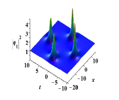
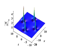
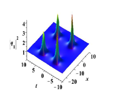
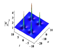
Figure 1: (color online) (a,b) The “rhombus” structure for the second-order vector RW which contains four fundamental ones. The parameters are $f_{1}=0,f_{2}=0,g_{1}=1,g_{2}=0,h_{1}=0,h_{2}=10000$ , (c,d) The “rectangle” structure for the second-order vector RW which contains four fundamental ones. The parameters are $f_{1}=0,f_{2}=0,g_{1}=1,g_{2}=1000,h_{1}=10,h_{2}=0$ .

The compact solution formula (9) can be used to derive N-th order RW solution. With $N=1$, the first order vector RW can be derived directly, which agrees well with the ones in Ling3 ; zhao2 . We find the dynamics structure of high order RW in the coupled system are much more abundant than the ones in scalar systems Yang ; Ling ; He ; Ling2 ; Akhmediev . Even for the second-order RW, whose distributions processes many different structures, which are quite different from the second order scalar ones. As an example, we exhibit the dynamics behavior of second order vector RW solution. Since the expressions of high order RW solution are quite complicated, we will present them elsewhere.

The dynamics of second order vector rogue waves— There are six free parameters in the generalized second order rogue wave solution, denoted by $f_{j}$, $g_{j}$ and $h_{j}$ ($j=1,2$), which can be used to obtain different types or patterns for the rogue wave dynamics. We find that there are mainly two kinds of rogue wave solutions which correspond to four fundamental RWs and six fundamental ones obtained by setting $f_{1}=0$ and $f_{1}\neq 0$ respectively.

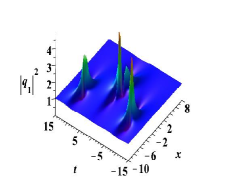
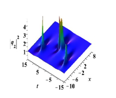
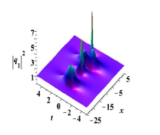
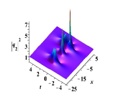
Figure 2: (color online) (a,b) The “triangle” structure for the second-order vector RW which contains four fundamental ones. The parameters are $f_{1}=0,f_{2}=100,g_{1}=1,g_{2}=0,h_{1}=0,h_{2}=0$, (c,d) The “line” structure for the second-order vector RW which contains four fundamental ones. The parameters are $f_{1}=0,f_{2}=0,g_{1}=1,g_{2}=0,h_{1}=10,h_{2}=0$.

Firstly, we discuss the second order RW solution which possesses four fundamental RWs. The pattern is quite different from the ones in scalar NLS systems Ling2 ; Akhmediev , for which it is impossible for four fundamental RWs to emerge on the temporal-spatial distribution plane. To obtain this kind of solution, we merely need to choose parameter $f_{1}=0$. We classify them by parameters $f_{2},g_{1},g_{2},h_{1},h_{2}$ whether or not are zeros. By this classification, there could be $2^{5}$ kinds of different solution which correspond to different patterns on the temporal-spatial distribution. In fact, the solution with different parameters here correspond to different ideal initial excitation for RW experimentally. We find there are mainly three types of the patterns, such as quadrilateral, triangle, and line structures.

The explicit shape of the quadrilateral can be varied though the parameters. As an example, we show two cases for the quadrilateral structure in Fig. 1. The first case: the four RWs arrange with the “rhombus” structure (Fig. 1(a,b)). The spatial-temporal distribution are similar globally in the two components, but the RW with highest peak emerge at different time, it appear at time $t=-5$ for the component $q_{1}$; and at $t=5$ for the component $q_{2}$. The second case: the four RWs arrange with “rectangle” structure (Fig. 1(c,d)). It is seen that the peak values of two RWs on the right hand is much higher than the ones on the left hand in the component $q_{1}$. The character is inverse for the component $q_{2}$.

Varying the other parameters, we can observe the interaction between the four RWs. When two of them fuse into be a new RW, the three RWs can emerge with “triangle” structure on the temporal-spatial distribution (Fig. 2(a,b)). The structure of the triangle can be changed by vary the parameters. Especially, the three RWs can emerge in a “line” (Fig. 2(c,d)), which is perpendicular with the $t$ axes. Namely, at a certain time, three or four RWs can emerge synchronously.

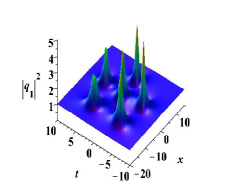
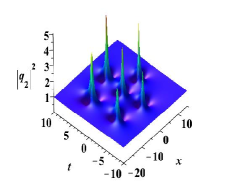
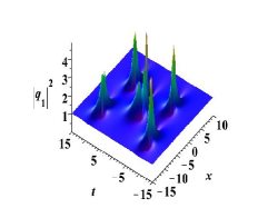
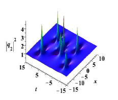
Figure 3: (color online) (a,b)The “pentagon” structure for the second-order vector RW which contains six fundamental ones. The parameters are $f_{1}=1,f_{2}=0,g_{1}=0,g_{2}=0,h_{1}=0,h_{2}=10000$ , (c,d) The “rectangle” structure for the second-order vector RW which contains six fundamental ones. The parameters are $f_{1}=1,f_{2}=0,g_{1}=0,g_{2}=0,h_{1}=100,h_{2}=0$.

Secondly, we consider the second case of second order RW solutions, which possess six fundamental RWs. To obtain this kind of solution, we choose the parameter $f_{1}=1$. One can simply classify this solution $2^{5}$ types by parameters $f_{2},g_{1},g_{2},h_{1},h_{2}$. But the six fundamental RWs can constitute many different structures, such as “pentagon”, “quadrilateral”, “triangle”, and “line” structures. As an example, we show the “pentagon” structure in Fig. 3(a,b). The pentagon structure can be varied too though changing the parameters. There is one RW in the internal region of the pentagon, and its location in the distribution plane can be varied too. This case is similar to the “pentagon” structure of the third order RW of scalar NLS equation Ling2 ; Akhmediev . The six RWs can be arranged with the “rectangle” structure through varying the parameters, such as the one in Fig. 3(c,d). The structure is similar to the one in Fig. 1(c,d). But there is a new RW insider “rectangle”, which is formed by the interaction of the other two fundamental RWs.

Similar to the ones for four fundamental RWs case, the six RWs can be arranged with the “triangle” structure too, such as the ones in Fig. 4(a,b). In this case, there are two fundamental RWs and a new RW to form a triangle. The new RW is formed by the interaction between the other four fundamental RWs. Moreover, the RWs can be arranged with “line” structure too, shown in Fig. 4(c,d). There should be six fundamental RWs arranged in one line case, but it is very complicated to derive the case since the parameters are too many to be managed well. We just show a particular one of the “line” cases.

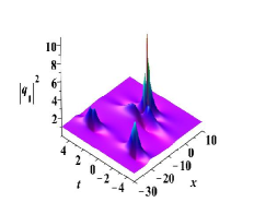
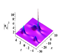
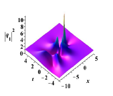
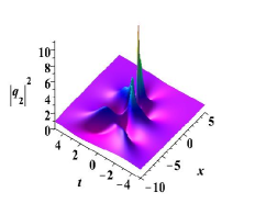
Figure 4: (color online) (a,b) The “triangle” structure for the second-order vector RW which contains six fundamental ones. The parameters are $f_{1}=1,f_{2}=0,g_{1}=10,g_{2}=0,h_{1}=0,h_{2}=0$ . (c,d) The “line” structure for the second-order vector RW which contains six fundamental ones. The parameters are $f_{1}=1,f_{2}=0,g_{1}=0,g_{2}=0,h_{1}=0,h_{2}=0$.

Possibilities to observe these vector rogue waves— Considering the experiments on RW in nonlinear fibers with anomalous GVD Kibler ; Solli , which have shown that the simple scalar NLS could describe nonlinear waves in nonlinear fibers well, we expect that these different vector nonlinear waves could be observed in two-mode nonlinear fibers. Consider the case that the operation wavelength of each mode is nearly $1.55\ \mu m$, the GVD coefficients are $-20\ ps^{2}km^{-1}$ in the anomalous regime, and the Kerr coefficients are nearly $1.1\ W^{-1}km^{-1}$, corresponding to the self-focusing effect in the fiber Dudley2 . The unit in $x$ direction will be denoted as $0.23\ ps$, and the one in $t$ will be denoted as $0.55\ km$. We discuss the proper conditions to observe the vector RWs. One can introduce two distinct modes to the nonlinear fiber operating in the anomalous GVD regime Afanasyev ; Ueda . The spontaneous development of RW seeded from some perturbation should be on the continuous waves as the ones in Kibler ; Solli . The continuous wave background intensities in the two modes should be equal (assume to be $30\ W$). The frequency difference between the two mode should be $0.23\ ps^{-1}$. Then the ideal initial optical shape can be given by the exact second-order vector RW solution with explicit coefficients in the scaled units. As shown in Kibler , the Peregrine RW characteristics can appear with initial conditions that do not correspond to the mathematical ideal, the vector RWs could be observed in the nonlinear fiber with approaching the ideal initial excitation form.

Conclusions— We find that there are mainly two kinds of rogue wave solutions for the second order vector RW in two-component coupled NLSE, which correspond to four fundamental RWs and six fundamental ones obtained by setting $f_{1}=0$ and $f_{1}\neq 0$ respectively. The distribution patten for vector RWs are much abundant than the ones for scalar rogue waves. These results could be helpful to understand the complex RW phenomena.

References

- (1) M. Onorato, S. Residori, U. Bortolozzo, A. Montina and F. T. Arecchi, Phys. Rep. 528, 47-89 (2013).
- (2) C. Kharif, E. Pelinovsky, and A. Slunyaev, Rogue Waves in the Ocean (Springer, Heidelberg, 2009).
- (3) A.R. Osborne, Nonlinear Ocean Waves and the Inverse Scattering Transform (Elsevier, New York, 2010).
- (4) V. Ruban, Y. Kodama, M. Ruderma, et al., Eur. Phys. Journ. Special Topics 185, 5-15 (2010).
- (5) N. Akhmediev and E. Pelinovsky, Eur. Phys. J. Special Topics 185, 1 (2010).
- (6) C. Kharif and E. Pelinovsky, Eur. J. Mech. B/Fluids 22, 603 (2003).
- (7) E. Pelinovsky and C. Kharif, Extreme Ocean Waves (Springer, Berlin, 2008).
- (8) D.R. Solli, C. Ropers, P. Koonath, B. Jalali, Nature 450, 06402 (2007).
- (9) B. Kibler, J. Fatome, C. Finot, G. Millot, et al., Nature Phys. 6, 790 (2010)..
- (10) A. Chabchoub, N.P. Hoffmann, and N. Akhmediev, Phys. Rev. Lett. 106, 204502 (2011).
- (11) H. Bailung, S.K. Sharma, and Y. Nakamura, Phys. Rev. Lett. 107, 255005 (2011).
- (12) A. R. Osborne, Mar. Struct. 14, 275 (2001); N. Akhmediev, A. Ankiewicz, M. Taki, Phys. Lett. A 373, 675-678 (2009).
- (13) N. Akhmediev, A. Ankiewicz, J.M. Soto-Crespo, Phys. Rev. E 80 026601 (2009); N. Akhmediev, A. Ankiewicz, J.M. Soto-Crespo, and J.M. Dudley, Phys. Lett. A 375, 541-544 (2011).
- (14) Y. Ohta, J.K. Yang, Proc. R. Soc. A 468, 1716-1740 (2012).
- (15) B.L. Guo, L.M. Ling, Q. P. Liu , Phys. Rev. E 85, 026607 (2012); B.L. Guo, L.L. Ling and Q. P. Liu, Stud. Appl. Math. 130, 317-344 (2013).
- (16) J. S. He, H. R. Zhang, L. H. Wang, K. Porsezian, and A. S. Fokas, Phys. Rev. E 87, 052914 (2013).
- (17) L.M. Ling, L.C. Zhao, Phys. Rev. E 88, 043201 (2013).
- (18) D.J. Kedziora, A. Ankiewicz, and N. Akhmediev, Phys. Rev. E 88, 013207 (2013).
- (19) C. Becker, S. Stellmer, P. S. Panahi, S. Dorscher, M. Baumert, E.-M. Richter, J. Kronjager, K. Bongs, and K. Sengstock, Nat. Phys. 4, 496 C501 (2008).
- (20) C. Hamner, J. J. Chang, P. Engels, and M. A. Hoefer, Phys. Rev. Lett. 106, 065302 (2011).
- (21) D. Y. Tang, H. Zhang, L. M. Zhao, and X. Wu, Phys. Rev. Lett. 101, 153904 (2008).
- (22) O.C. Wright, M.G. Forest, Physica D 141, 104 C116 (2000); M.G. Forest, S.P. Sheu, and P.C. Wright, Phys. Lett. A 266, 24-33 (2000).
- (23) M.G. Forest, O.C. Wright, Physica D 178, 173-189 (2003).
- (24) K.W. Chow, K.K.Y. Wong, K. Lam, Phys. Lett. A 372, 4596-4600 (2008).
- (25) Y.V. Bludov, V.V. Konotop, and N. Akhmediev, Eur. Phys. J. Special Topics 185, 169 (2010).
- (26) L.C. Zhao and J. Liu, J. Opt. Soc. Am. B 29, 3119-3127 (2012).
- (27) F. Baronio, A. Degasperis, M. Conforti, and S. Wabnitz, Phys. Rev. Lett. 109, 044102 (2012).
- (28) B.L. Guo, L.M. Ling, Chin. Phys. Lett. 28, 110202 (2011).
- (29) L.C. Zhao and J. Liu, Phys. Rev. E 87, 013201 (2013).
- (30) F. Baronio, M. Conforti, A. Degasperis, and S. Lombardo, Phys. Rev. Lett. 111, 114101 (2013).
- (31) A.Chabchoub,N.Akhmediev, Phys. Lett. A 377, 2590-2593(2013).
- (32) A. Chabchoub, N. Hoffmann, M. Onorato, A. Slunyaev, A. Sergeeva, E. Pelinovsky, and N. Akhmediev, Phys. Rev. E 86, 056601 (2012).
- (33) M. Erkintalo, K. Hammani, B. Kibler, C. Finot, N. Akhmediev, J.M. Dudley, and G. Genty, Phys. Rev. Lett. 107, 253901 (2011).
- (34) J. M. Dudley, G. Genty, F. Dias, B. Kibler, N. Akhmediev, Opt. Express 17, 21497-21508 (2009).
- (35) B. Crosignani and P. Di Porto, Opt. Lett. 6, 329 (1981); V. V. Afanasyev, Yu. S. Kivshar, V. V. Konotop, V. N. Serkin, Opt. Lett. 14, 805 (1989).
- (36) Tetsuji Ueda and William L. Lath, Phys. Rev. A 42, 563 (1990).