Dirichlet-Neumann and Neumann-Neumann Waveform Relaxation Algorithms for Parabolic Problems

Abstract

We present and analyze a waveform relaxation version of the Dirichlet-Neumann and Neumann-Neumann methods for parabolic problems. Like the Dirichlet-Neumann method for steady problems, the method is based on a non-overlapping spatial domain decomposition, and the iteration involves subdomain solves with Dirichlet boundary conditions followed by subdomain solves with Neumann boundary conditions. For the Neumann-Neumann method, one step of the method consists of solving the subdomain problems using Dirichlet interface conditions, followed by a correction step involving Neumann interface conditions. However, each subdomain problem is now in space and time, and the interface conditions are also time-dependent. Using Laplace transforms, we show for the heat equation that when we consider finite time intervals, the Dirichlet-Neumann and Neumann-Neumann methods converge superlinearly for an optimal choice of the relaxation parameter, similar to the case of Schwarz waveform relaxation algorithms. The convergence rate depends on the size of the subdomains as well as the length of the time window. For any other choice of the relaxation parameter, convergence is only linear. We illustrate our results with numerical experiments.

1 Introduction

We introduce and analyze new types of Waveform Relaxation (WR) methods based on the Dirichlet-Neumann and Neumann-Neumann algorithms for steady problems. To solve time-dependent problems in parallel, one can either discretize in time to obtain a sequence of steady problems, which is called Rothe’s method after the German analyst Erich Rothe, and then one applies domain decomposition algorithms to solve the steady problems at each time step in parallel. Or one can first discretize in space, which is called the method of lines, and then apply WR to the large system of ordinary differential equations (ODEs) obtained from the spatial discretization. WR methods have their origin in the work of Picard [27] and Lindelöf [18] for the existence proof of solutions of ODEs in the late 19th century. Lelarasmee, Ruehli and Sangiovanni-Vincentelli [17] were the first to introduce WR as a parallel method for the solution of ODEs. For WR methods applied to ODEs, we have two classical convergence results: (i) linear convergence on unbounded time intervals under some dissipation assumptions on the splitting ([24], [25], [15] and [23]); and (ii) superlinear convergence for nonlinear systems (including linear ones) on bounded time intervals, assuming a Lipschitz condition on the splitting function ([24], [25], [1] and [3]). The main computational advantage of the WR method next to parallelization is that one can use different time discretizations for different components of the system.

Domain decomposition methods for elliptic PDEs can be extended to time dependent problems by using the same decomposition in space, but then solving time dependent problems in the subdomains during the iterative solution process. This leads to WR type methods, see the early references [3] and [15]. The systematic extension of the classical Schwarz method to time dependent problems was started independently in [13, 14]; Gander and Stuart [13] showed linear convergence of overlapping Schwarz WR iteration for the heat equation on unbounded time intervals with a rate depending on the size of the overlap; Giladi and Keller [14] proved superlinear convergence of the Schwarz WR method with overlap on bounded time intervals for the convection-diffusion equation. Like WR algorithms in general, the so called Schwarz Waveform Relaxation algorithms (SWR) converge relatively slowly, except if the time window size is very short. A remedy is to use optimized transmission conditions, which leads to much faster algorithms, see [11, 2] for parabolic problems, and [12, 10] for hyperbolic problems, and this technique also led to the so called optimized Schwarz methods for elliptic problems, for an overview, see [9].

The Dirichlet-Neumann and Neumann-Neumann methods belong to the class of substructuring methods for solving elliptic PDEs. The Dirichlet-Neumann algorithm was first considered by Bjørstad & Widlund [4] and further studied in [6], [22] and [21]; the Neumann-Neumann algorithm was introduced by Bourgat et al. [5], see also [29] and [31]. The performance of these algorithms for elliptic problems is now well understood, see for example the book [32]. However, no substructuring-type analogue of the WR method has been proposed so far. In this paper, we propose the Dirichlet-Neumann Waveform Relaxation (DNWR) and the Neumann-Neumann Waveform Relaxation (NNWR) methods, which generalize the use of substructuring methods to the case of time-dependent problems in a natural way. We define and analyze these methods in the continuous setting to ensure the understanding of the asymptotic behavior of the methods in the case of fine grids.

We formulate the new algorithms for the following parabolic equation on a bounded domain $\Omega\subset\mathbb{R}^{d}$, $0<t<T$, $d=1,2,3$:

$$\begin{array}[]{rcll}\displaystyle\frac{\partial u}{\partial t}&=&\nabla\cdot\left(\kappa(\boldsymbol{x},t)\nabla u\right)+f(\boldsymbol{x},t),&\boldsymbol{x}\in\Omega,\ 0<t<T,\\ u(\boldsymbol{x},0)&=&u_{0}(\boldsymbol{x}),&\boldsymbol{x}\in\Omega,\\ u(\boldsymbol{x},t)&=&g(\boldsymbol{x},t),&\boldsymbol{x}\in\partial\Omega,\ 0<t<T,\end{array}$$ (1)

where $\kappa(\boldsymbol{x},t)\geq\kappa>0$. In Section 2, we introduce the non-overlapping DNWR algorithm with two subdomains for the model problem (1), and we present sharp convergence estimates for DNWR obtained for the special case of the one dimensional heat equation, $\kappa(\boldsymbol{x},t)=1$. In Section 3 we present the NNWR algorithm for multiple subdomains for the general problem (1), and present sharp convergence estimates again for the one dimensional heat equation. Our convergence analysis shows that both the DNWR and NNWR algorithms converge superlinearly on finite time intervals, $T<\infty$. It is based on detailed, technical kernel estimates, which we show in Section 4. Section 5 contains the proofs of our main convergence results for both DNWR and NNWR. We then show in Section 6 how the analysis of the NNWR can be generalized to higher spatial dimensions, and prove that the convergence estimates do not change. We finally show numerical results in Section 7, which illustrate our analysis. We also test the algorithms in configurations not covered by our analysis, and still observe the same convergence behavior.

2 The Dirichlet-Neumann Waveform Relaxation algorithm

To define the Dirichlet-Neumann WR algorithm for the model problem (1) on the space-time domain $\Omega\times(0,T)$ with Dirichlet data given on $\partial\Omega$, we assume that the spatial domain $\Omega$ is partitioned into two non-overlapping subdomains $\Omega_{1}$ and $\Omega_{2}$, as illustrated in Figure 1.

Fig. 1: Splitting into two non-overlapping subdomains

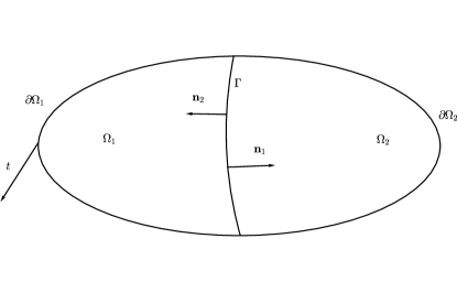
We denote by $u_{i}$ the restriction of the solution $u$ of (1) to $\Omega_{i}$, $i=1,2$, and by $\boldsymbol{n}_{i}$ the unit outward normal for $\Omega_{i}$ on the interface $\Gamma:=\partial\Omega_{1}\cap\partial\Omega_{2}$. The Dirichlet-Neumann Waveform Relaxation algorithm consists of the following steps: given an initial guess $h^{0}(\boldsymbol{x},t)$ along the interface $\Gamma\times(0,T)$, compute for $k=1,2,\ldots$ with $u_{1}^{k}=g$ on $\partial\Omega_{1}\setminus\Gamma$ and $u_{2}^{k}=g$ on $\partial\Omega_{2}\setminus\Gamma$ the approximations

$$\begin{array}[]{rcll}\partial_{t}u_{1}^{k}-\nabla\cdot\left(\kappa(\boldsymbol{x},t)\nabla u_{1}^{k}\right)&=&f,&\textrm{in}\;\Omega_{1},\\ u_{1}^{k}(\boldsymbol{x},0)&=&u_{0}(\boldsymbol{x}),&\textrm{in}\;\Omega_{1},\\ u_{1}^{k}&=&h^{k-1},&\textrm{on}\;\Gamma,\end{array}\ \begin{array}[]{rcll}\partial_{t}u_{2}^{k}-\nabla\cdot\left(\kappa(\boldsymbol{x},t)\nabla u_{2}^{k}\right)&=&f,&\textrm{in}\;\Omega_{2},\\ u_{2}^{k}(\boldsymbol{x},0)&=&u_{0}(\boldsymbol{x}),&\textrm{in}\;\Omega_{2},\\ \partial_{\boldsymbol{n}_{2}}u_{2}^{k}&=&-\partial_{\boldsymbol{n}_{1}}u_{1}^{k},&\textrm{on}\;\Gamma,\end{array}$$ (2)

and then update the value along the interface using

$$h^{k}(\boldsymbol{x},t)=\theta u_{2}^{k}\left|{}_{\Gamma\times(0,T)}\right.+(1-\theta)h^{k-1}(\boldsymbol{x},t),$$ (3)

$\theta\in(0,1]$ being a relaxation parameter. Now the main goal of the analysis is to study how the error $h^{k-1}(\boldsymbol{x},t)-u\left|{}_{\Gamma\times(0,T)}\right.$ converges to zero, and by linearity it suffices to consider the so called error equations, $f(\boldsymbol{x},t)=0$, $g(\boldsymbol{x},t)=0$, $u_{0}(\boldsymbol{x})=0$ in (2), and examine how $h^{k-1}(\boldsymbol{x},t)$ converges to zero as $k\rightarrow\infty$.

We present now sharp convergence estimates for algorithm (2,3) for the special case of the heat equation, $\kappa(\boldsymbol{x},t)=1$, on the one dimensional domain $\Omega=(-a,b)$ with subdomains $\Omega_{1}=(-a,0)$ and $\Omega_{2}=(0,b)$. Our convergence analysis is based on Laplace transforms. We define the Laplace transform of a function $u(x,t)$ with respect to time $t$ as

$$\hat{u}(x,s):=\mathcal{L}\left\{u(x,t)\right\}:=\int_{0}^{\infty}e^{-st}u(x,t)\,dt,$$ (4)

where $s$ is a complex variable. If $\mathcal{L}\left\{u(x,t)\right\}=\hat{u}(x,s)$, then the inverse Laplace transform of $\hat{u}(x,s)$ is defined by

$$\mathcal{L}^{-1}\left\{\hat{u}(x,s)\right\}:=u(x,t),\qquad t\geq 0,$$ (5)

and maps the Laplace transform of a function back to the original function. For more information on Laplace transforms, see [8, 26].

After a Laplace transform, the DNWR algorithm (2,3) for the error equations in the one dimensional heat equation setting becomes

$$\begin{array}[]{rcll}(s-\partial_{xx})\hat{u}_{1}^{k}&=&0&\textrm{on $(-a,0)$},\\ \hat{u}_{1}^{k}(-a,s)&=&0,\\ \hat{u}_{1}^{k}(0,s)&=&\hat{h}^{k-1}(s),\end{array}\quad\begin{array}[]{rcll}(s-\partial_{xx})\hat{u}_{2}^{k}&=&0&\textrm{on $(0,b)$},\\ \partial_{x}\hat{u}_{2}^{k}(0,s)&=&\partial_{x}\hat{u}_{1}^{k}(0,s),\\ \hat{u}_{2}^{k}(b,s)&=&0,\end{array}$$ (6)

followed by the updating step

$$\hat{h}^{k}(s)=\theta\hat{u}_{2}^{k}(0,s)+(1-\theta)\hat{h}^{k-1}(s).$$ (7)

Solving the two-point boundary value problems in the Dirichlet and Neumann step in (6), we get

$$\hat{u}_{1}^{k}(x,s) = \frac{\hat{h}^{k-1}(s)}{\sinh(a\sqrt{s})}\sinh\left((x+a)\sqrt{s}\right),$$ (8)

$$\hat{u}_{2}^{k}(x,s) = \hat{h}^{k-1}(s)\frac{\coth(a\sqrt{s})}{\cosh(b\sqrt{s})}\sinh((x-b)\sqrt{s}).$$ (9)

By induction, we therefore find for the updating step the relation

$$\hat{h}^{k}(s)=\left(1-\theta-\theta\tanh(b\sqrt{s})\coth(a\sqrt{s})\right)^{k}\hat{h}^{0}(s),\quad k=1,2,3,\ldots$$ (10)

Theorem 1 (Convergence of DNWR for $a=b$).

When the subdomains are of the same size, $a=b$ in (6,7), the DNWR algorithm converges linearly for $0<\theta<1$, $\theta\neq 1/2$. For $\theta=1/2$, it converges in two iterations. Convergence is independent of the time window size $T$.

Proof.

For $a=b$, equation (10) reduces to $\hat{h}^{k}(s)=(1-2\theta)^{k}\hat{h}^{0}(s),$ which has the simple back transform $h^{k}(t)=(1-2\theta)^{k}h^{0}(t)$. Thus the convergence is linear for $0<\theta<1$, $\theta\neq 1/2$. If $\theta=1/2$, we have $h^{1}(t)=0$, and hence one more iteration produces the desired solution on the entire domain. ∎

Having treated the simple case where the subdomains are of the same size, $a=b$, we focus now on the more interesting case where $a\neq b$. Defining

$$G(s):=\tanh(b\sqrt{s})\coth(a\sqrt{s})-1=\frac{\sinh((b-a)\sqrt{s})}{\sinh(a\sqrt{s})\cosh(b\sqrt{s})},$$ (11)

the recurrence relation (10) can be rewritten as

$$\hat{h}^{k}(s)=\left\{\begin{array}[]{ll}\left(q(\theta)-\theta G(s)\right)^{k}\hat{h}^{0}(s),&\theta\neq 1/2,\\ \left(-1\right)^{k}2^{-k}G^{k}(s)\hat{h}^{0}(s),&\theta=1/2,\end{array}\right.$$ (12)

where $q(\theta)=1-2\theta$. Note that for $\textrm{Re}(s)>0,$ $G(s)$ is $\mathcal{O}(s^{-p})$ for every positive $p$, which can be seen as follows: setting $s=re^{i\vartheta}$, we obtain for $a\geq b$ the bound

$$\left|s^{p}G(s)\right|\leq\left|\frac{s^{p}}{\cosh(b\sqrt{s})}\right|\leq\frac{2r^{p}}{\left|e^{b\sqrt{r/2}}-e^{-b\sqrt{r/2}}\right|}\rightarrow 0\quad\mbox{as $r\rightarrow\infty$},$$

and for $a<b$, we get the bound

$$\left|s^{p}G(s)\right|\leq\left|\frac{s^{p}}{\sinh(a\sqrt{s})}\right|\leq\frac{2r^{p}}{\left|e^{a\sqrt{r/2}}-e^{-a\sqrt{r/2}}\right|}\rightarrow 0\quad\mbox{as $r\rightarrow\infty$}.$$

Therefore, by [8, p. 178], $G(s)$ is the Laplace transform of an infinitely differentiable function $F_{1}(t)$, which is the reason why we introduced $G(s)$ in (11). We now define $F_{k}(t):=\mathcal{L}^{-1}\left\{G^{k}(s)\right\}$ for $k=1,2,3,\ldots$. In what follows, we study the special case $\theta=1/2$, when $h^{k}$ is given by a convolution of $h^{0}$ with the analytic function $F_{k}$. For $\theta$ not equal to $1/2$, different techniques are required to analyze the behavior of the DNWR algorithm, and this will be done in a future paper. We also have to consider two cases: $a>b$, which means that the Dirchlet subdomain is bigger than Neumann subdomain, and $a<b$, when the Neumann subdomain is bigger than the Dirichlet subdomain. We have the following two convergence results, whose proofs will be given in Section 5.

Theorem 2 (Convergence of DNWR for $a>b$).

If $\theta=1/2$ and the Dirichlet subdomain is larger than the Neumann subdomain, then the error of the DNWR algorithm (6,7) satisfies for $t\in(0,\infty)$ the linear convergence estimate

$$\|h^{k}\|_{L^{\infty}(0,\infty)}\leq\left(\frac{a-b}{2a}\right)^{k}\|h^{0}\|_{L^{\infty}(0,\infty)}.$$ (13)

On a finite time interval $t\in(0,T)$, the DNWR method converges superlinearly with the estimate

$$\|h^{k}\|_{L^{\infty}(0,T)}\leq\left(\frac{a-b}{a}\right)^{k}\operatorname{erfc}\left(\frac{kb}{2\sqrt{T}}\right)\|h^{0}\|_{L^{\infty}(0,T)}.$$ (14)

Theorem 3 (Convergence of DNWR for $a<b$).

If $\theta=1/2$ and the Dirichlet subdomain is smaller than the Neumann subdomain, then the error of the DNWR algorithm (6,7) satisfies for $t\in(0,\infty)$ the linear convergence estimate

$$\|h^{2k}\|_{L^{\infty}(0,\infty)}\leq\left(\frac{b-a}{2a}\right)^{2k}\|h^{0}\|_{L^{\infty}(0,\infty)}.$$ (15)

For a finite time interval $t\in(0,T)$, the DNWR converges superlinearly with the estimate

$$\|h^{2k}\|_{L^{\infty}(0,T)}\leq\left(\frac{\sqrt{2}}{1-e^{-\frac{(2k+1)a^{2}}{T}}}\right)^{2k}e^{-k^{2}a^{2}/T}\|h^{0}\|_{L^{\infty}(0,T)}.$$ (16)

Remark 4.

The linear estimate (15) does not always imply convergence, because $b-a$ can be larger than $2a$. In other words, when $b>3a$, i.e., when the Neumann subdomain is much larger than the Dirichlet one, the error over the infinite time interval does not converge to zero as $k\to\infty$. In this case, one should switch the interface conditions and solve a Dirichlet problem on the larger subdomain.

3 The Neumann-Neumann Waveform Relaxation algorithm

We now introduce the NNWR algorithm for the model problem (1) for multiple subdomains; for the case of two subdomains in 1d, see [16]. Suppose $\Omega$ is partitioned into non-overlapping subdomains $\{\Omega_{i}$, $1\leq i\leq N\}$, as illustrated in Figure 2.

Fig. 2: Splitting into many non-overlapping subdomains

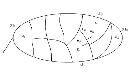
For $i=1,\ldots,N$ set $\Gamma_{i}:=\partial\Omega_{i}\setminus\partial\Omega$, $\Lambda_{i}:=\{j\in\{1,\ldots,N\}:\Gamma_{i}\cap\Gamma_{j}\,\mbox{has nonzero measure}\}$ and $\Gamma_{ij}:=\partial\Omega_{i}\cap\partial\Omega_{j}$, so that the interface of $\Omega_{i}$ can be rewritten as $\Gamma_{i}=\bigcup_{j\in\Lambda_{i}}\Gamma_{ij}$. We denote by $\boldsymbol{n}_{ij}$ the unit outward normal for $\Omega_{i}$ on the interface $\Gamma_{ij}$.

The NNWR algorithm starts with an initial guess $w_{ij}^{0}(\boldsymbol{x},t)$ along the interfaces $\Gamma_{ij}\times(0,T)$, $j\in\Lambda_{i}$, $i=1,\ldots,N$, and then performs the following two-step iteration: at each iteration $k$, one first solves Dirichlet problem on each $\Omega_{i}$ in parallel,

$$\begin{array}[]{rcll}\partial_{t}u_{i}^{k}-\nabla\cdot\left(\kappa(\boldsymbol{x},t)\nabla u_{i}^{k}\right)&=&f,&\mbox{in $\Omega_{i}$},\\ u_{i}^{k}(\boldsymbol{x},0)&=&u_{0}(\boldsymbol{x}),&\mbox{in $\Omega_{i}$},\\ u_{i}^{k}&=&g,&\mbox{on $\partial\Omega_{i}\setminus\Gamma_{i}$},\\ u_{i}^{k}&=&w_{ij}^{k-1},&\mbox{on $\Gamma_{ij},j\in\Lambda_{i}$}.\end{array}$$ (17)

One then solves Neumann problems on all subdomains,

$$\begin{array}[]{rcll}\partial_{t}\psi_{i}^{k}-\nabla\cdot\left(\kappa(\boldsymbol{x},t)\nabla\psi_{i}^{k}\right)&=&0,&\mbox{in $\Omega_{i}$},\\ \psi_{i}^{k}(\boldsymbol{x},0)&=&0,&\mbox{in $\Omega_{i}$},\\ \psi_{i}^{k}&=&0,&\mbox{on $\partial\Omega_{i}\setminus\Gamma_{i}$},\\ \partial_{\boldsymbol{n}_{ij}}\psi_{i}^{k}&=&\partial_{\boldsymbol{n}_{ij}}u_{i}^{k}+\partial_{\boldsymbol{n}_{ji}}u_{j}^{k},&\mbox{on $\Gamma_{ij},j\in\Lambda_{i}$}.\end{array}$$ (18)

The interface values are then updated with the formula

$$w_{ij}^{k}(\boldsymbol{x},t)=w_{ij}^{k-1}(\boldsymbol{x},t)-\theta\left(\psi_{i}^{k}\left|{}_{\Gamma_{ij}\times(0,T)}\right.+\psi_{j}^{k}\left|{}_{\Gamma_{ij}\times(0,T)}\right.\right),$$ (19)

where $\theta\in(0,1]$ is a relaxation parameter.

As in the case of the DNWR algorithm, we prove our results first for the one dimensional heat equation on the domain $\Omega:=(0,L)$ with boundary conditions $u(0,t)=g_{0}(t)$ and $u(L,t)=g_{L}(t)$, for higher spatial dimensions, see Section 6. We decompose $\Omega$ into non-overlapping subdomains $\Omega_{i}:=(x_{i-1},x_{i})$, $i=1,\ldots,N$, and define the subdomain length $h_{i}:=x_{i}-x_{i-1}$, and $h_{\min}:=\min_{1\leq i\leq N}h_{i}$. Our initial guess is denoted by $\left\{w_{i}^{0}(t)\right\}_{i=1}^{N-1}$ on the interfaces $x_{i}$. By linearity, we again study the error equations, $f=0$, $g_{0}=g_{L}=0$ and $u_{0}=0$, which leads with $w_{0}^{k}(t)=w_{N}^{k}(t)=0$ for all $k$ to

$$\begin{array}[]{rclrcl}\partial_{t}u_{i}^{k}-\partial_{xx}u_{i}^{k}&=&0,\qquad\textrm{in $\Omega_{i}$},&\partial_{t}\psi_{i}^{k}-\partial_{xx}\psi_{i}^{k}&=&0,\qquad\textrm{in $\Omega_{i}$},\\ u_{i}^{k}(x,0)&=&0,\qquad\textrm{in $\Omega_{i}$},&\psi_{i}^{k}(x,0)&=&0,\qquad\textrm{in $\Omega_{i}$},\\ u_{i}^{k}(x_{i-1},t)&=&w_{i-1}^{k-1}(t),&-\partial_{x}\psi_{i}^{k}(x_{i-1},t)&=&(\partial_{x}u_{i-1}^{k}-\partial_{x}u_{i}^{k})(x_{i-1},t),\\ u_{i}^{k}(x_{i},t)&=&w_{i}^{k-1}(t),&\partial_{x}\psi_{i}^{k}(x_{i},t)&=&(\partial_{x}u_{i}^{k}-\partial_{x}u_{i+1}^{k})(x_{i},t),\end{array}$$ (20)

except for the first and last subdomain, where in the Neumann step the Neumann conditions are replaced by homogeneous Dirichlet conditions along the physical boundaries. The new interface values for the next step are then defined as

$$w_{i}^{k}(t)=w_{i}^{k-1}(t)-\theta\left(\psi_{i}^{k}(x_{i},t)+\psi_{i+1}^{k}(x_{i},t)\right).$$ (21)

We have the following convergence result for NNWR:

Theorem 5 (Convergence of NNWR).

For $\theta=1/4$ and $T>0$ fixed, the NNWR algorithm (20)–(21) converges superlinearly with the estimate

$$\max_{1\leq i\leq N-1}\|w_{i}^{k}\|_{L^{\infty}(0,T)}\leq\left(\frac{\sqrt{6}}{1-e^{-\frac{(2k+1)h_{\min}^{2}}{T}}}\right)^{2k}e^{-k^{2}h_{\min}^{2}/T}\max_{1\leq i\leq N-1}\|w_{i}^{0}\|_{L^{\infty}(0,T)}.$$ (22)

The proof of Theorem 5 will also be given in Section 5. As in the case of the DNWR, the parameter choice $\theta\neq 1/4$ requires different analysis techniques and is the subject of further studies.

4 Kernel estimates

The convergence results given in Theorems 2, 3 and 5 are based on technical estimates of kernels arising in the Laplace transform of the DNWR and NNWR algorithms. We present in this section the precise estimates needed.

4.1 Properties of Laplace transforms

We start with several elementary properties of positive functions and their Laplace transforms.

Lemma 6.

Let $g$ and $w$ be two real-valued functions in $(0,\infty)$ with $\hat{w}(s)=\mathcal{L}\left\{w(t)\right\}$ the Laplace transform of $w$. Then for $t\in(0,T)$, we have the following properties:

1. If $g(t)\geq 0$ and $w(t)\geq 0$, the convolution $(g*w)(t):=\int_{0}^{t}g(t-\tau)w(\tau)d\tau\geq 0$.

2. $\|g*w\|_{L^{1}(0,T)}\leq\|g\|_{L^{1}(0,T)}\|w\|_{L^{1}(0,T)}.$

3. $\bigl{|}(g*w)(t)\bigl{|}\leq\|g\|_{L^{\infty}(0,T)}\int_{0}^{T}\bigl{|}w(\tau)\bigl{|}d\tau.$

4. $\int_{0}^{t}w(\tau)d\tau=(H*w)(t)=\mathcal{L}^{-1}\left(\frac{\hat{w}(s)}{s}\right)$, $H(t)$ being the Heaviside step function.

Proof.

The proofs follow directly from the definitions. ∎

Lemma 7.

Let, $w(t)$ be a continuous and $L^{1}$-integrable function on $(0,\infty)$ with $w(t)\geq 0$ for all $t\geq 0$, and $\hat{w}(s)=\mathcal{L}\left\{w(t)\right\}$ be its Laplace transform. Then, for $\tau>0$, we have the bound

$$\int_{0}^{\tau}|w(t)|dt\leq\lim_{s\rightarrow 0+}\hat{w}(s).$$ (23)

Proof.

With the definition of the Laplace transform (4) and using positivity, we have

$$\int_{0}^{\tau}|w(t)|dt = \int_{0}^{\tau}w(t)dt\leq\int_{0}^{\infty}w(t)dt=\int_{0}^{\infty}\lim_{s\rightarrow 0+}e^{-st}w(t)dt$$

$$= \lim_{s\rightarrow 0+}\int_{0}^{\infty}e^{-st}w(t)dt=\lim_{s\rightarrow 0+}\hat{w}(s),$$

where the dominated convergence theorem was used to exchange the order of limit and integration. ∎

4.2 Positivity

In order to use Lemma 7 in our analysis, we have to show positivity of inverse transforms of kernels appearing in the DNWR and NNWR iteration. These results are established in the following lemma.

Lemma 8.

Let $\beta>\alpha\geq 0$ and $s$ be a complex variable. Then, for $t\in(0,\infty)$

$$\varphi(t):=\mathcal{L}^{-1}\left\{\frac{\sinh(\alpha\sqrt{s})}{\sinh(\beta\sqrt{s})}\right\}\geq 0\quad\mbox{and}\quad\psi(t):=\mathcal{L}^{-1}\left\{\frac{\cosh(\alpha\sqrt{s})}{\cosh(\beta\sqrt{s})}\right\}\geq 0.$$

Proof.

We first prove that $\varphi$ and $\psi$ are well-defined and continous functions on $(0,\infty)$. Setting $s=re^{i\vartheta}$, a short calculation shows that for $\beta>\alpha\geq 0$ and for every positive $p$

$$\left|\frac{s^{p}\sinh(\alpha\sqrt{s})}{\sinh(\beta\sqrt{s})}\right|\leq r^{p}\cdot\left|\frac{e^{\alpha\sqrt{r/2}}+e^{-\alpha\sqrt{r/2}}}{e^{\beta\sqrt{r/2}}-e^{-\beta\sqrt{r/2}}}\right|\to 0\qquad\text{as $r\to\infty$,}$$

so by [8, p. 178], its inverse Laplace transform exists and is continuous (in fact, infinitely differentiable). Thus, $\varphi$ is a continuous function. A similar argument holds for $\psi$.

Next, we prove the positivity of $\varphi$ and $\psi$ by noting that these kernels are related to solutions of the heat equation. Let us consider the heat equation $u_{t}-u_{xx}=0$ on $(0,\beta)$ with initial condition $u(x,0)=0$ and boundary conditions $u(0,t)=0$, $u(\beta,t)=g(t)$. If $g$ is non-negative, then by the maximum principle, this boundary value problem has a non-negative solution $u(\alpha,t)$ for all $\alpha\in[0,\beta]$, $t>0$. Now performing a Laplace transform of the heat equation in time, we obtain the transformed solution along $x=\alpha$ to be

$$\hat{u}(\alpha,s)=\hat{g}(s)\frac{\sinh(\alpha\sqrt{s})}{\sinh(\beta\sqrt{s})}\quad\Longrightarrow\quad u(\alpha,t)=\int_{0}^{t}g(t-\tau)\varphi(\tau)d\tau.$$

We now prove that $\varphi(t)\geq 0$ by contradiction: suppose $\varphi(t_{0})<0$ for some $t_{0}>0$. Then by the continuity of $\varphi$, there exists $\delta>0$ such that $\varphi(\tau)<0$ for $\tau\in(t_{0}-\delta,t_{0}+\delta)$. Now for $t>t_{0}+\delta,$ we choose a non-negative $g$ as follows:

$$g(\zeta)=\begin{cases}1,&\zeta\in\left(t-t_{0}-\delta,t-t_{0}+\delta\right)\\ 0,&\textrm{otherwise}.\end{cases}$$

Then $u(\alpha,t)=\int_{t_{0}-\delta}^{t_{0}+\delta}g(t-\tau)\varphi(\tau)d\tau=\int_{t_{0}-\delta}^{t_{0}+\delta}\varphi(\tau)d\tau<0$, which is a contradiction, and hence $\varphi$ must be non-negative. To prove the result for $\psi$, we use again the heat equation $u_{t}-u_{xx}=0$, $u(x,0)=0$, but on the domain $(-b,b)$ and with boundary conditions $u(-\beta,t)=u(\beta,t)=g(t)$. Using a Laplace transform in time gives as solution at $x=\alpha$

$$\hat{u}(\alpha,s)=\hat{g}(s)\frac{\cosh(\alpha\sqrt{s})}{\cosh(\beta\sqrt{s})},$$

and hence a similar argument as in the first case proves that $\psi$ is also non-negative. ∎

4.3 Specific kernel estimates

The following lemma contains specific estimates for the inverse Laplace transform of two kernels in terms of infinite sums.

Lemma 9.

For $k=1,2,3,\ldots$, we have the identities

$$\mathcal{L}^{-1}\left(\operatorname{cosech}^{k}(\alpha\sqrt{s})\right) = 2^{k}{\displaystyle\sum_{m=0}^{\infty}}\binom{m+k-1}{m}\frac{(2m+k)\alpha}{\sqrt{4\pi t^{3}}}e^{-(2m+k)^{2}\alpha^{2}/4t},$$ (24)

$$\mathcal{L}^{-1}\left(\frac{\operatorname{cosech}^{k}(\alpha\sqrt{s})}{s}\right) = 2^{k}{\displaystyle\sum_{m=0}^{\infty}}\binom{m+k-1}{m}\operatorname{erfc}\left(\frac{(2m+k)\alpha}{2\sqrt{t}}\right).$$ (25)

In particular, both functions are positive for $t>0$.

Proof.

Using that $\bigl{|}e^{-2\alpha\sqrt{s}}\bigl{|}<1$ for $\mbox{Re}(s)>0$, we first expand cosech into an infinite binomial series,

$$\textrm{cosech}^{k}(\alpha\sqrt{s}) =\left(\frac{2}{e^{\alpha\sqrt{s}}-e^{-\alpha\sqrt{s}}}\right)^{k}=2^{k}e^{-k\alpha\sqrt{s}}\left(1-e^{-2\alpha\sqrt{s}}\right)^{-k}$$

$$=2^{k}{\displaystyle\sum_{m=0}^{\infty}}\binom{m+k-1}{m}e^{-(2m+k)\alpha\sqrt{s}}.$$ (26)

Now using the inverse Laplace transform (see Oberhettinger [26])

$$\mathcal{L}^{-1}\left(e^{-\lambda\sqrt{s}}\right)=\frac{\lambda}{\sqrt{4\pi t^{3}}}e^{-\lambda^{2}/4t},\quad\lambda>0,$$ (27)

we obtain

$$\mathcal{L}^{-1}\left(\text{cosech}^{k}(\alpha\sqrt{s})\right) = 2^{k}\sum_{m=0}^{\infty}\binom{m+k-1}{m}\mathcal{L}^{-1}\left(e^{-(2m+k)\alpha\sqrt{s}}\right)$$ (28)

$$= 2^{k}\sum_{m=0}^{\infty}\binom{m+k-1}{m}\frac{(2m+k)\alpha}{\sqrt{4\pi t^{3}}}e^{-(2m+k)^{2}\alpha^{2}/4t}.$$

To justify taking the inverse Laplace transform term by term, we prove that the Laplace transform of the right-hand side of (28) indeed gives $\operatorname{cosech}^{k}(\alpha\sqrt{s})$. Let $f_{m}(t)=2^{k}{m+k-1\choose m}\frac{(2m+k)\alpha}{\sqrt{4\pi t^{3}}}e^{-(2m+k)^{2}\alpha^{2}/4t}$ be the $m$th term of the series. Then for any real parameter $s_{0}>0$, we have for $\textrm{Re}(s)>s_{0}$

$$\int_{0}^{\infty}|e^{-st}f_{m}(t)|\,dt \leq 2^{k}\int_{0}^{\infty}e^{-s_{0}t}{m+k-1\choose m}\frac{(2m+k)\alpha}{\sqrt{4\pi t^{3}}}e^{-(2m+k)^{2}\alpha^{2}/4t}\,dt$$

$$=2^{k}{m+k-1\choose m}e^{-(2m+k)\alpha\sqrt{s_{0}}}.$$

Thus, we have

$$\sum_{m=0}^{\infty}\int_{0}^{\infty}|e^{-st}f_{m}(t)|\,dt\leq\operatorname{cosech}^{k}(\alpha\sqrt{s_{0}})<\infty.$$

This allows us to use Fubini’s theorem, where the product measure is between the discrete counting measure and the Lebesgue measure on $[0,\infty)$. We thus obtain for all $\textrm{Re}(s)\geq s_{0}$

$$\int_{0}^{\infty}e^{-st}\sum_{m=0}^{\infty}f_{m}(t)\,dt=\sum_{m=0}^{\infty}\int_{0}^{\infty}e^{-st}f_{m}(t)\,dt=\operatorname{cosech}^{k}(\alpha\sqrt{s}).$$

The first identity (24) then follows by taking the inverse Laplace transform on both sides. Since each $f_{m}(t)$ is positive for $t>0$, we conclude that the limit function $\sum_{m=0}^{\infty}f_{m}(t)$ is also positive.

For the second identity, we need the inverse Laplace transform

$$\mathcal{L}^{-1}\left(\frac{1}{s}e^{-\lambda\sqrt{s}}\right)=\textrm{erfc}\left(\frac{\lambda}{2\sqrt{t}}\right),\quad\lambda>0.$$ (29)

By dividing the expansion (26) by $s$, we obtain

$$\mathcal{L}^{-1}\left(\frac{\text{cosech}^{k}(\alpha\sqrt{s})}{s}\right) = 2^{k}\sum_{m=0}^{\infty}\binom{m+k-1}{m}\mathcal{L}^{-1}\left(\frac{1}{s}e^{-(2m+k)\alpha\sqrt{s}}\right)$$ (30)

$$= 2^{k}\sum_{m=0}^{\infty}\binom{m+k-1}{m}\textrm{erfc}\left(\frac{(2m+k)\alpha}{2\sqrt{t}}\right),$$

where we justify the interchanging of sums and inverse transforms in the same way as above. Since $\operatorname{erfc}$ is a positive function, so is the kernel (25). ∎

5 Proofs of the main theorems

We now prove the main convergence results for the DNWR and NNWR algorithms stated in Section 2 and 3.

5.1 Proof of Theorem 2 for DNWR

For $\theta=1/2$ we get from (12) and using part 3 of Lemma 6

$$\left|h^{k}(t)\right|=\left|2^{-k}(-1)^{k}\left(h^{0}*F_{k}\right)(t)\right|\leq 2^{-k}\|h^{0}\|_{L^{\infty}(0,T)}\int_{0}^{T}\left|F_{k}(\tau)\right|d\tau.$$ (31)

So in order to get an $L^{\infty}$ convergence estimate, we need to bound $\int_{0}^{T}\left|F_{k}(\tau)\right|d\tau$. Now in Theorem 2, $a>b$, and $\mathcal{L}\left(-F_{1}(t)\right)=\frac{\sinh((a-b)\sqrt{s})}{\sinh(a\sqrt{s})}\cdot\frac{1}{\cosh(b\sqrt{s})}$. So by Lemma 7 and the fact that the convolution of two positive functions is positive, see Lemma 6 point 1, $-F_{1}(t)$ is positive. Thus, $(-1)^{k}F_{k}(t)\geq 0$ for all $t$, and we obtain from Lemma 7

$$\int_{0}^{T}\left|(-1)^{k}F_{k}(\tau)\right|d\tau\leq\lim_{s\rightarrow 0+}(-1)^{k}G^{k}(s)=\left(\frac{a-b}{a}\right)^{k}.$$

This bound is valid for arbitrary values of $T$, and hence we get from (31)

$$\|h^{k}\|_{L^{\infty}(0,\infty)}\leq\left(\frac{a-b}{2a}\right)^{k}\|h^{0}\|_{L^{\infty}(0,\infty)},$$

which shows that the algorithm is converging at least linearly for $a>b$. To get a more accurate bound, we define $\hat{v}^{k}(s):=\cosh^{k}(b\sqrt{s})\hat{h}^{k}(s)$, and rewrite (12) for $\theta=1/2$ as

$$\hat{v}^{k}(s)=2^{-k}\frac{\sinh^{k}((a-b)\sqrt{s})}{\sinh^{k}(a\sqrt{s})}\hat{v}^{0}(s).$$

So if we set $g_{k}(t):=\mathcal{L}^{-1}\left(\frac{\sinh^{k}((a-b)\sqrt{s})}{\sinh^{k}(a\sqrt{s})}\right)$, then part 3 of Lemma 6 yields

$$\|v^{k}\|_{L^{\infty}(0,T)}\leq 2^{-k}\|v^{0}\|_{L^{\infty}(0,T)}\int_{0}^{T}|g_{k}(\tau)|d\tau.$$

By Lemma 7, $\int_{0}^{T}g_{k}(\tau)d\tau\leq\left(\frac{a-b}{a}\right)^{k}$, and we therefore obtain

$$\|v^{k}\|_{L^{\infty}(0,T)}\leq\left(\frac{a-b}{2a}\right)^{k}\|v^{0}\|_{L^{\infty}(0,T)}.$$ (32)

Setting $f_{k}(t):=\mathcal{L}^{-1}\left(\frac{1}{\cosh^{k}(b\sqrt{s})}\right)$ we have

$$h^{k}(t)=\left(f_{k}*v^{k}\right)(t)=\int_{0}^{t}f_{k}(t-\tau)v^{k}(\tau)d\tau,$$

from which it follows, using again part 3 of Lemma 6 that

$$\|h^{k}\|_{L^{\infty}(0,T)}\leq\|v^{k}\|_{L^{\infty}(0,T)}\int_{0}^{T}|f_{k}(\tau)|d\tau.$$ (33)

By Lemma 8, $f_{k}(t)\geq 0$ for all $t$. To obtain a bound for $\int_{0}^{T}f_{k}(\tau)\,d\tau$, we first show that the function $r_{k}(t)=\mathcal{L}^{-1}(2^{k}e^{-kb\sqrt{s}})$ is greater than or equal to $f_{k}(t)$ for all $t>0$, and then bound $\int_{0}^{T}r_{k}(\tau)\,d\tau$ instead. Indeed, we have

$$\mathcal{L}\left\{r_{k}(t)-f_{k}(t)\right\} =2^{k}e^{-kb\sqrt{s}}-\frac{2^{k}}{(e^{b\sqrt{s}}+e^{-b\sqrt{s}})^{k}}$$

$$=\frac{2^{k}((1+e^{-2b\sqrt{s}})^{k}-1)}{(e^{b\sqrt{s}}+e^{-b\sqrt{s}})^{k}}$$

$$=\sum_{j=1}^{k}{k\choose j}e^{-2jb\sqrt{s}}\operatorname{sech}^{k}(b\sqrt{s}).$$

Note that in addition to $f_{k}(t)=\mathcal{L}^{-1}(\operatorname{sech}^{k}(b\sqrt{s}))$, $\mathcal{L}^{-1}(e^{-2jb\sqrt{s}})$ is also a positive function for $j=1,\ldots,k$; see (27). Thus, $\mathcal{L}^{-1}(e^{-2jb\sqrt{s}}\operatorname{sech}^{k}(b\sqrt{s}))$ is a convolution of positive functions, and hence positive by part 1 of Lemma 6. This implies $r_{k}(t)-f_{k}(t)\geq 0$, so we deduce that

$$\int_{0}^{T}f_{k}(\tau)\,d\tau\leq\int_{0}^{T}r_{k}(\tau)\,d\tau=\mathcal{L}^{-1}\left(\frac{2^{k}e^{-kb\sqrt{s}}}{s}\right)=2^{k}\,\textrm{erfc}\left(\frac{kb}{2\sqrt{T}}\right),$$

where we expressed the second integral as an inverse Laplace transform using Lemma 6, part 4, which we then evaluated using (29). Finally, we combine the bound above with (32) and (33) to obtain the second estimate of Theorem 2, which concludes the proof of this theorem.

5.2 Proof of Theorem 3 for DNWR

For the case $a<b$, a linear estimate which does not depend on $T$ has been given in [20]. For the second part, we rewrite (12) in the form

$$\hat{h}^{2k}(s)=\left(-\frac{1}{2}\right)^{2}G(s)\hat{h}^{2k-1}(s)=\frac{1}{4}G^{2}(s)\hat{h}^{2k-2}(s),$$ (34)

and defining $\hat{\phi}(s):=\frac{\sinh^{2}((b-a)\sqrt{s})}{\cosh^{2}(b\sqrt{s})}$, $\hat{h}_{1}(s)=\frac{\cosh^{2}((b-a)\sqrt{s})}{\cosh^{2}(b\sqrt{s})}$ and $\hat{h}_{2}(s)=\frac{1}{\cosh^{2}(b\sqrt{s})}$, we can rewrite

$$G^{2}(s)=\frac{\sinh^{2}((b-a)\sqrt{s})}{\sinh^{2}(a\sqrt{s})\cosh^{2}(b\sqrt{s})}=\frac{1}{\sinh^{2}(a\sqrt{s})}\hat{\phi}(s)=\frac{1}{\sinh^{2}(a\sqrt{s})}\left(\hat{h}_{1}(s)-\hat{h}_{2}(s)\right).$$

This motivates the definition of the new sequence $\hat{\vartheta}^{2k}(s):=\sinh^{2k}(a\sqrt{s})\hat{h}^{2k}(s)$, which from (34) satisfies the recurrence

$$\hat{\vartheta}^{2k}(s)=\frac{1}{4}\hat{\phi}(s)\hat{\vartheta}^{2k-2}(s).$$

Now using part 3 of Lemma 6, we obtain the estimate

$$\|\vartheta^{2k}\|_{L^{\infty}(0,T)}\leq\frac{1}{4}\|\vartheta^{2k-2}\|_{L^{\infty}(0,T)}\int_{0}^{T}|\phi(\tau)|d\tau,$$ (35)

and using Lemma 7 leads to

$$\int_{0}^{T}|\phi(\tau)|d\tau \leq \int_{0}^{T}h_{1}(\tau)d\tau+\int_{0}^{T}h_{2}(\tau)d\tau$$

$$\leq \lim_{s\rightarrow 0+}\frac{\cosh^{2}((b-a)\sqrt{s})}{\cosh^{2}(b\sqrt{s})}+\lim_{s\rightarrow 0+}\frac{1}{\cosh^{2}(b\sqrt{s})}=2.$$

By induction, we therefore obtain

$$\|\vartheta^{2k}\|_{L^{\infty}(0,T)}\leq\frac{1}{2^{k}}\|\vartheta^{0}\|_{L^{\infty}(0,T)}=\frac{1}{2^{k}}\|h^{0}\|_{L^{\infty}(0,T)}.$$ (36)

Now defining $\varphi_{2k}(t)=\mathcal{L}^{-1}\left(\frac{1}{\sinh^{2k}(a\sqrt{s})}\right)$, we have

$$h^{2k}(t)=\left(\varphi_{2k}*\vartheta^{2k}\right)(t)=\int_{0}^{t}\varphi_{2k}(t-\tau)\vartheta^{2k}(\tau)d\tau,$$

from which it follows by part 3 of Lemma 6 and using (36) that

$$\|h^{2k}\|_{L^{\infty}(0,T)}\leq\|\vartheta^{2k}\|_{L^{\infty}(0,T)}\int_{0}^{T}|\varphi_{2k}(\tau)|d\tau\leq B(k,T)\|h^{0}\|_{L^{\infty}(0,T)},$$ (37)

where $B(k,T):=\frac{1}{2^{k}}\int_{0}^{T}|\varphi_{2k}(\tau)|d\tau$. By Lemma 9, $\varphi_{2k}(t)\geq 0$ for all $t>0$. Thus by part 4 of Lemma 6, and then using equation (25) from Lemma 9, we get

$$B(k,T) = \frac{1}{2^{k}}\mathcal{L}^{-1}\left(\frac{\textrm{cosech}^{2k}(a\sqrt{s})}{s}\right)_{t=T}$$

$$= 2^{k}\sum_{m=0}^{\infty}\binom{m+2k-1}{m}\textrm{erfc}\left(\frac{(m+k)a}{\sqrt{T}}\right)$$

$$\leq 2^{k}\sum_{m=0}^{\infty}\binom{m+2k-1}{m}\exp\left(-\frac{(m+k)^{2}a^{2}}{T}\right)$$

$$= 2^{k}e^{-k^{2}a^{2}/T}\sum_{m=0}^{\infty}\binom{m+2k-1}{m}\exp\left(-\frac{(m^{2}+2km)a^{2}}{T}\right)$$

$$\leq 2^{k}e^{-k^{2}a^{2}/T}\sum_{m=0}^{\infty}\binom{m+2k-1}{m}\exp\left(-\frac{m(2k+1)a^{2}}{T}\right)$$

$$\leq \left(\frac{\sqrt{2}}{1-e^{-\frac{2k+1}{\sigma}}}\right)^{2k}e^{-k^{2}/\sigma},\quad\textrm{with $\sigma:=T/a^{2}$},$$

where we used for the first inequality the estimate

$$\textrm{erfc}(x)=\frac{2}{\sqrt{\pi}}\int_{x}^{\infty}e^{-t^{2}}dt=\frac{2}{\sqrt{\pi}}\int_{0}^{\infty}e^{-(x+t)^{2}}dt\leq\frac{2}{\sqrt{\pi}}e^{-x^{2}}\int_{0}^{\infty}e^{-t^{2}}dt\leq e^{-x^{2}},$$

and for the third inequality

$$\frac{1}{(1-z)^{\beta}}=\sum_{m\geq 0}\binom{m+\beta-1}{m}z^{m},\quad\mbox{for $|z|<1$}.$$

Inserting the estimate for $B(k,T)$ into (37) gives then the result of the theorem.

Remark 10.

Note that the factor multiplying $e^{-k^{2}a^{2}/T}$ in the estimate (16) is an increasing function of $k$ in general, since $\frac{\sqrt{2}}{1-e^{-\frac{2k+1}{\sigma}}}>1$. Thus, the bound (16) may increase initially for small iteration numbers $k$, before the factor $e^{-k^{2}a^{2}/T}$ starts dominating and causing the bound to decrease to zero superlinearly. To estimate the turning point, let us fix an integer $l>0$ and consider the behavior of the algorithm for iteration numbers $k>2l$. Then by writing $\alpha=e^{-l/\sigma}$, we can bound $B(k,T)$ by

$$B(k,T) =\left(\frac{\sqrt{2}}{1-e^{-\frac{2k+1}{\sigma}}}\right)^{2k}e^{-2kl/\sigma}e^{-k(k-2l)/\sigma}$$

$$\leq\left(\frac{\sqrt{2}e^{-l/\sigma}}{1-e^{-\frac{2k}{\sigma}}}\right)^{2k}e^{-k(k-2l)/\sigma}\leq{\underbrace{\left(\frac{\sqrt{2}\alpha}{1-\alpha^{4}}\right)}_{=(*)}}^{2k}e^{-\frac{(k-2l)^{2}}{\sigma}}.$$

Thus, if $\sqrt{2}\alpha/(1-\alpha^{4})<1$, then the factor ($*$) is less than 1 and the bound $B(k,T)$ contracts superlinearly for $k>2l$. This is true whenever $\alpha<\alpha_{0}$, where $\alpha_{0}\approx 0.6095$ is the unique positive root of $\psi(\alpha)=\alpha^{4}+\sqrt{2}\alpha-1$. Hence, we get superlinear convergence for $k>2l>0.99T/a^{2}.$

5.3 Proof of Theorem 5 for NNWR

We start by applying the Laplace transform to the homogeneous Dirichlet subproblems in (20), and obtain

$$s\hat{u}_{i}-\hat{u}_{i,xx}=0,\quad\hat{u}_{i}(x_{i-1},s)=\hat{w}_{i-1}(s),\quad\hat{u}_{i}(x_{i},s)=\hat{w}_{i}(s),$$

for $i=2,...,N-1.$ These subdomain problems have the solutions

$$\hat{u}_{i}(x,s)=\frac{1}{\sinh(h_{i}\sqrt{s})}\left(\hat{w}_{i}(s)\sinh\left((x-x_{i-1})\sqrt{s}\right)+\hat{w}_{i-1}(s)\sinh\left((x_{i}-x)\sqrt{s}\right)\right).$$

Next we apply the Laplace transform to the Neumann subproblems (18) for subdomains not touching the physical boundary, and obtain

$$\hat{\psi}_{i}(x,s)=C_{i}(s)\cosh\left((x-x_{i-1})\sqrt{s}\right)+D_{i}(s)\cosh\left((x_{i}-x)\sqrt{s}\right),$$

where the notation $\sigma_{i}:=\sinh\left(h_{i}\sqrt{s}\right)$ and $\gamma_{i}:=\cosh\left(h_{i}\sqrt{s}\right)$ gives

$$C_{i} = \frac{1}{\sigma_{i}}\left(\hat{w}_{i}\left(\frac{\gamma_{i}}{\sigma_{i}}+\frac{\gamma_{i+1}}{\sigma_{i+1}}\right)-\frac{\hat{w}_{i-1}}{\sigma_{i}}-\frac{\hat{w}_{i+1}}{\sigma_{i+1}}\right),$$

$$D_{i} = \frac{1}{\sigma_{i}}\left(\hat{w}_{i-1}\left(\frac{\gamma_{i}}{\sigma_{i}}+\frac{\gamma_{i-1}}{\sigma_{i-1}}\right)-\frac{\hat{w}_{i-2}}{\sigma_{i-1}}-\frac{\hat{w}_{i}}{\sigma_{i}}\right).$$

We therefore obtain for $i=2,...,N-2,$ at iteration $k$

$$\hat{w}_{i}^{k}(s) = \hat{w}_{i}^{k-1}(s)-\theta\left(\hat{\psi}_{i}^{k}(x_{i},s)+\hat{\psi}_{i+1}^{k}(x_{i},s)\right)$$

$$= \hat{w}_{i}^{k-1}(s)-\theta\left(C_{i}\gamma_{i}+D_{i}+C_{i+1}+D_{i+1}\gamma_{i+1}\right).$$

Using the identity $\gamma_{i}^{2}-1=\sigma_{i}^{2}$ and simplifying, we get

$$\begin{array}[]{rcl}\hat{w}_{i}^{k}&=&\displaystyle\hat{w}_{i}^{k-1}-\theta\left(\hat{w}_{i}^{k-1}\left(2+\frac{2\gamma_{i}\gamma_{i+1}}{\sigma_{i}\sigma_{i+1}}\right)+\frac{\hat{w}_{i+1}^{k-1}}{\sigma_{i+1}}\left(\frac{\gamma_{i+2}}{\sigma_{i+2}}-\frac{\gamma_{i}}{\sigma_{i}}\right)\right.\\ &&\hskip 40.00006pt\displaystyle\left.+\frac{\hat{w}_{i-1}^{k-1}}{\sigma_{i}}\left(\frac{\gamma_{i-1}}{\sigma_{i-1}}-\frac{\gamma_{i+1}}{\sigma_{i+1}}\right)-\frac{\hat{w}_{i+2}^{k-1}}{\sigma_{i+1}\sigma_{i+2}}-\frac{\hat{w}_{i-2}^{k-1}}{\sigma_{i}\sigma_{i-1}}\right).\end{array}$$ (38)

For $i=1$ and $i=N$, the Neumann conditions on the physical boundary are replaced by homogeneous Dirichlet conditions $\psi_{1}(0,t)=0$ and $\psi_{N}(L,t)=0$, $t>0$. For these two subdomains, we obtain as solution after a Laplace transform

$$\hat{\psi}_{1}(x,s) = \frac{1}{\gamma_{1}}\left(\hat{w}_{1}\left(\frac{\gamma_{1}}{\sigma_{1}}+\frac{\gamma_{2}}{\sigma_{2}}\right)-\frac{\hat{w}_{2}}{\sigma_{2}}\right)\sinh\left((x-x_{0})\sqrt{s}\right),$$

$$\hat{\psi}_{N}(x,s) = \frac{1}{\gamma_{N}}\left(\hat{w}_{N-1}\left(\frac{\gamma_{N-1}}{\sigma_{N-1}}+\frac{\gamma_{N}}{\sigma_{N}}\right)-\frac{\hat{w}_{N-2}}{\sigma_{N-1}}\right)\sinh\left((x_{N}-x)\sqrt{s}\right),$$

and thus the recurrence relations on the first interface is

$$\hat{w}_{1}^{k}=\hat{w}_{1}^{k-1}-\theta\left(\hat{w}_{1}^{k-1}\left(2+\frac{\gamma_{1}\gamma_{2}}{\sigma_{1}\sigma_{2}}+\frac{\sigma_{1}\gamma_{2}}{\gamma_{1}\sigma_{2}}\right)+\frac{\hat{w}_{2}^{k-1}}{\sigma_{2}}\left(\frac{\gamma_{3}}{\sigma_{3}}-\frac{\sigma_{1}}{\gamma_{1}}\right)-\frac{\hat{w}_{3}^{k-1}}{\sigma_{2}\sigma_{3}}\right),$$ (39)

and on the last interface, we obtain

$$\begin{array}[]{rcl}\hat{w}_{N-1}^{k}&=&\displaystyle\hat{w}_{N-1}^{k-1}-\theta\left(\hat{w}_{N-1}^{k-1}\left(2+\frac{\gamma_{N-1}\gamma_{N}}{\sigma_{N-1}\sigma_{N}}+\frac{\sigma_{N}\gamma_{N-1}}{\gamma_{N}\sigma_{N-1}}\right)\right.\\ &&\displaystyle\left.\hskip 50.00008pt+\frac{\hat{w}_{N-2}^{k-1}}{\sigma_{N-1}}\left(\frac{\gamma_{N-2}}{\sigma_{N-2}}-\frac{\sigma_{N}}{\gamma_{N}}\right)-\frac{\hat{w}_{N-3}^{k-1}}{\sigma_{N-1}\sigma_{N-2}}\right).\end{array}$$ (40)

Defining $\sigma:=\sinh(h_{\min}\sqrt{s})$ where $h_{\min}=\min_{1\leq i\leq N}h_{i}$, and setting

$$\hat{\nu}_{i}^{k}(s):=\sigma^{2k}\hat{w}_{i}^{k}(s),$$ (41)

relation (38) reduces for the special choice $\theta=1/4$ to

$$\hat{\nu}_{i}^{k}(s)=-\frac{1}{4}\left(\hat{t}_{i,i}\hat{\nu}_{i}^{k-1}(s)+\hat{t}_{i,i+1}\hat{\nu}_{i+1}^{k-1}(s)+\hat{t}_{i,i-1}\hat{\nu}_{i-1}^{k-1}(s)-\hat{t}_{i,i+2}\hat{\nu}_{i+2}^{k-1}(s)-\hat{t}_{i,i-2}\hat{\nu}_{i-2}^{k-1}(s)\right),$$ (42)

where we defined $\hat{t}_{i,i}:=\frac{2\sigma^{2}}{\sigma_{i}\sigma_{i+1}}(\gamma_{i}\gamma_{i+1}-\sigma_{i}\sigma_{i+1})$, $\hat{t}_{i,i+1}:=\frac{\sigma^{2}}{\sigma_{i}\sigma_{i+1}\sigma_{i+2}}(\sigma_{i}\gamma_{i+2}-\gamma_{i}\sigma_{i+2})$, $\hat{t}_{i,i-1}:=\frac{\sigma^{2}}{\sigma_{i}\sigma_{i-1}\sigma_{i+1}}(\sigma_{i+1}\gamma_{i-1}-\gamma_{i+1}\sigma_{i-1})$, $\hat{t}_{i,i+2}:=\frac{\sigma^{2}}{\sigma_{i+1}\sigma_{i+2}}$, and $\hat{t}_{i,i-2}:=\frac{\sigma^{2}}{\sigma_{i}\sigma_{i-1}}$. Similarly, we obtain for (39)

$$\hat{\nu}_{1}^{k}(s)=-\frac{1}{4}\left(\hat{t}_{1,1}\hat{\nu}_{1}^{k-1}(s)+\hat{t}_{1,2}\hat{\nu}_{2}^{k-1}(s)-\hat{t}_{1,3}\hat{\nu}_{3}^{k-1}(s)\right),$$ (43)

where we defined $\hat{t}_{1,1}:=\sigma^{2}\left(\frac{\sigma_{1}\gamma_{2}}{\gamma_{1}\sigma_{2}}+\frac{\gamma_{1}\gamma_{2}}{\sigma_{1}\sigma_{2}}-2\right)$, $\hat{t}_{1,2}=\frac{\sigma^{2}}{\sigma_{2}}\left(\frac{\gamma_{3}}{\sigma_{3}}-\frac{\sigma_{1}}{\gamma_{1}}\right)$ and $\hat{t}_{1,3}=\frac{\sigma^{2}}{\sigma_{2}\sigma_{3}}$. From (40), we obtain

$$\hat{\nu}_{N-1}^{k}(s)=-\frac{1}{4}\left(\hat{t}_{N-1,N-1}\hat{\nu}_{N-1}^{k-1}(s)+\hat{t}_{N-1,N-2}\hat{\nu}_{N-2}^{k-1}(s)-\hat{t}_{N-1,N-3}\hat{\nu}_{N-3}^{k-1}(s)\right),$$ (44)

where we defined $\hat{t}_{N-1,N-1}:=\sigma^{2}\left(\frac{\sigma_{N-1}\gamma_{N-2}}{\gamma_{N-1}\sigma_{N-2}}+\frac{\gamma_{N-1}\gamma_{N-2}}{\sigma_{N-1}\sigma_{N-2}}-2\right)$, $\hat{t}_{N-1,N-2}=\frac{\sigma^{2}}{\sigma_{N-2}}\left(\frac{\gamma_{N-3}}{\sigma_{N-3}}-\frac{\sigma_{N-1}}{\gamma_{N-1}}\right)$ and $\hat{t}_{N-1,N-3}=\frac{\sigma^{2}}{\sigma_{N-2}\sigma_{N-3}}$. Now we will show that for all $i$

$$\|\nu_{i}^{k}\|_{L^{\infty}(0,T)}\leq\frac{3}{2}\max_{1\leq j\leq N-1}\|\nu_{j}^{k-1}\|_{L^{\infty}(0,T)},\quad k=1,2,3,\ldots.$$ (45)

At first glance it seems that inequality (45) is not enough to prove convergence, because the factor $3/2$ is bigger than one, but the $\nu_{i}^{k}$ are related to the $w_{i}^{k}$ by $\sigma$, see (41), and the superlinear convergence of $w_{i}^{k}$ will come from $\sigma$. To obtain (45), we have to bound $\int_{0}^{\infty}|t_{i,j}(t)|dt$, where $t_{i,j}=\mathcal{L}^{-1}\left\{\hat{t}_{i,j}\right\}$. We first consider $\hat{t}_{i,i+2}$. If $h_{i+1}=h_{i+2}=h_{\min}$, then the terms in $\hat{t}_{i,i+2}$ cancel and we simply get $\hat{t}_{i,i+2}=1$. If $h_{\min}\leq h_{i+1}$ and $h_{\min}\leq h_{i+2}$, then the kernel $t_{i,i+2}$, being a convolution of two positive functions, is positive by part 1 of Lemma 6, and using Lemma 7 its integral is bounded by

$$\int_{0}^{\infty}|t_{i,i+2}(t)|dt\leq\lim_{s\rightarrow 0+}\frac{\sinh^{2}(h_{\min}\sqrt{s})}{\sinh(h_{i+1}\sqrt{s})\sinh(h_{i+2}\sqrt{s})}\leq\frac{h_{\min}^{2}}{h_{i+1}h_{i+2}}\leq 1,$$

so that

$$\|\mathcal{L}^{-1}\left(\hat{t}_{i,i+2}\hat{\nu}_{i+2}^{k}(s)\right)\|_{L^{\infty}(0,T)}\leq\|\nu_{i+2}^{k}\|_{L^{\infty}(0,T)}.$$

The same argument also holds for the term involving $\hat{\nu}_{i-2}^{k-1}$. Now for $\hat{\nu}_{i+1}^{k-1}$, we rewrite $\hat{t}_{i,i+1}$ as

$$\hat{t}_{i,i+1}=\frac{\sinh\left((h_{i}-h_{i+2})\sqrt{s}\right)\sinh^{2}(h_{\min}\sqrt{s})}{\sinh(h_{i}\sqrt{s})\sinh(h_{i+1}\sqrt{s})\sinh(h_{i+2}\sqrt{s})}.$$

Assuming that $h_{i}\geq h_{i+2}$, we use Lemma 8 and Lemma 7 to get a bound of the form

$$\int_{0}^{\infty}|t_{i,i+1}(t)|dt\leq\frac{|h_{i}-h_{i+2}|h_{\min}^{2}}{h_{i}h_{i+1}h_{i+2}}<1,$$

and similarly for the term involving $\hat{\nu}_{i-1}^{k-1}$. Finally, for the term $\hat{t}_{i,i}$, we use the trigonometric identity $\sinh(A)\cosh(B)=\frac{1}{2}\left(\sinh(A+B)+\sinh(A-B)\right)$ to obtain

$$\hat{t}_{i,i} = \frac{\sinh(h_{\min}\sqrt{s})\sinh\left((h_{\min}+h_{i}-h_{i+1})\sqrt{s}\right)}{\sinh(h_{i}\sqrt{s})\sinh(h_{i+1}\sqrt{s})}$$

$$+ \frac{\sinh(h_{\min}\sqrt{s})\sinh\left((h_{\min}+h_{i+1}-h_{i})\sqrt{s}\right)}{\sinh(h_{i}\sqrt{s})\sinh(h_{i+1}\sqrt{s})}.$$

Each term is again a ratio of hyperbolic sines, so we only need to pair the factors so that the coefficient in the numerator is always smaller than the one in the denominator. Now $-h_{i+1}\leq h_{\min}+h_{i}-h_{i+1}=h_{i}+h_{\min}-h_{i+1}\leq h_{i}$, so for the first term, we choose the pairing

$$\frac{\sinh(h_{\min}\sqrt{s})}{\sinh(h_{i+1}\sqrt{s})}\cdot\frac{\sinh\left((h_{\min}+h_{i}-h_{i+1})\sqrt{s}\right)}{\sinh(h_{i}\sqrt{s})}\quad\textrm{if}\;h_{i+1}\leq h_{i},$$

and

$$\frac{\sinh(h_{\min}\sqrt{s})}{\sinh(h_{i}\sqrt{s})}\cdot\frac{\sinh\left((h_{\min}+h_{i}-h_{i+1})\sqrt{s}\right)}{\sinh(h_{i+1}\sqrt{s})}\quad\textrm{if}\;h_{i+1}\geq h_{i}.$$

A similar argument holds also for the second term. Now using Lemma 7, we have again integrals of kernels bounded by 1. In summary, we get for $2\leq i\leq N-2$

$$\|\nu_{i}^{k}\|_{L^{\infty}(0,T)} \leq \frac{1}{2}\|\nu_{i}^{k-1}\|_{L^{\infty}(0,T)}+\frac{1}{4}\left(\|\nu_{i-2}^{k-1}\|_{L^{\infty}(0,T)}+\|\nu_{i-1}^{k-1}\|_{L^{\infty}(0,T)}\right.$$

$$\hskip 90.00014pt+\left.\|\nu_{i+1}^{k-1}\|_{L^{\infty}(0,T)}+\|\nu_{i+2}^{k-1}\|_{L^{\infty}(0,T)}\right),$$

and the estimate (45) is established for interior subdomains. For the left subdomain touching the boundary, the kernel $t_{1,3}$ in (43) can be estimated like $t_{i,i+2}$. For $\hat{t}_{1,2}$, we have

$$\hat{t}_{1,2}=\frac{\cosh\left((h_{1}-h_{3})\sqrt{s}\right)\sinh^{2}(h_{\min}\sqrt{s})}{\cosh(h_{1}\sqrt{s})\sinh(h_{2}\sqrt{s})\sinh(h_{3}\sqrt{s})}.$$

If $h_{1}\geq h_{3}$, the decomposition $\hat{t}_{1,2}=\frac{\cosh\left((h_{1}-h_{3})\sqrt{s}\right)}{\cosh(h_{1}\sqrt{s})}\cdot\frac{\sinh(h_{\min}\sqrt{s})}{\sinh(h_{2}\sqrt{s})}\cdot\frac{\sinh(h_{\min}\sqrt{s})}{\sinh(h_{3}\sqrt{s})}$ shows that one can bound

$$\int_{0}^{\infty}|t_{1,2}(t)|dt\leq h_{\min}^{2}/h_{2}h_{3}<1.$$

If $h_{3}>h_{1}$, then we rewrite

$$\hat{t}_{1,2} = \frac{1}{\cosh(h_{1}\sqrt{s})}\cdot\frac{\sinh(h_{\min}\sqrt{s})}{\sinh(h_{2}\sqrt{s})}\left(\frac{\sinh\left((h_{\min}+h_{1}-h_{3})\sqrt{s}\right)}{2\sinh(h_{3}\sqrt{s})}\right.$$

$$\hskip 130.0002pt\left.+\frac{\sinh\left((h_{\min}+h_{3}-h_{1})\sqrt{s}\right)}{2\sinh(h_{3}\sqrt{s})}\right),$$

which again shows using Lemma 7 that the integral is bounded by 1. Finally we consider

$$\hat{t}_{1,1} = \frac{2\cosh\left((2h_{1}-h_{2})\sqrt{s}\right)\sinh^{2}(h_{\min}\sqrt{s})}{\sinh(2h_{1}\sqrt{s})\sinh(h_{2}\sqrt{s})}$$

$$= \frac{\sinh(h_{\min}\sqrt{s})\sinh\left((h_{\min}+2h_{1}-h_{2})\sqrt{s}\right)}{\sinh(2h_{1}\sqrt{s})\sinh(h_{2}\sqrt{s})}+\frac{\sinh(h_{\min}\sqrt{s})\sinh\left((h_{\min}-2h_{1}+h_{2})\sqrt{s}\right)}{\sinh(2h_{1}\sqrt{s})\sinh(h_{2}\sqrt{s})}.$$

Using the inequalities $-h_{2}\leq h_{\min}+2h_{1}-h_{2}\leq 2h_{1}$ and $-2h_{1}\leq h_{\min}-2h_{1}+h_{2}\leq h_{2}$ we can again, with an appropriate pairing of factors, bound the integral of each term by 1. Thus we have for the subdomain touching the left physical boundary

$$\|\nu_{1}^{k}\|_{L^{\infty}(0,T)}\leq\frac{1}{2}\|\nu_{1}^{k-1}\|_{L^{\infty}(0,T)}+\frac{1}{4}\left(\|\nu_{2}^{k-1}\|_{L^{\infty}(0,T)}+\|\nu_{3}^{k-1}\|_{L^{\infty}(0,T)}\right).$$

A similar result holds for $\hat{\nu}_{N-1}^{k}(s)$, and hence the inequality (45) holds for all $1\leq i\leq N-1$. Therefore, by induction, we obtain

$$\max_{1\leq j\leq N-1}\|\nu_{j}^{k}\|_{L^{\infty}(0,T)}\leq\left(\frac{3}{2}\right)^{k}\max_{1\leq j\leq N-1}\|\nu_{j}^{0}\|_{L^{\infty}(0,T)}=\left(\frac{3}{2}\right)^{k}\max_{1\leq j\leq N-1}\|w_{j}^{0}\|_{L^{\infty}(0,T)}.$$

Now since

$$w_{i}^{k}(t)=\left(\phi_{2k}*\nu_{i}^{k}\right)(t)=\int_{0}^{t}\phi_{2k}(t-\tau)\nu_{i}^{k}(\tau)d\tau,$$

with $\phi_{2k}=\mathcal{L}^{-1}\left(\frac{1}{\sinh^{2k}(h_{\min}\sqrt{s})}\right)$, a similar estimate using part 3 of Lemma 6 as in the proof of Theorem 3 leads to the superlinear convergence estimate (22).

6 Analysis of the NNWR in 2D

In this section we formulate and analyze the NNWR algorithm, applied to the two-dimensional heat equation

$$\partial_{t}u-\Delta u=f(x,y,t),\quad(x,y)\in\Omega=(l,L)\times(0,\pi),\>t\in(0,T]$$

with initial condition $u(x,y,0)=u_{0}(x,y)$ and Dirichlet boundary conditions. To define the Neumann-Neumann algorithm, we decompose $\Omega$ into strips of the form $\Omega_{i}=(x_{i-1},x_{i})\times(0,\pi)$, $l=x_{0}<x_{1}<\cdots<x_{N}=L$. The Neumann-Neumann algorithm, considering directly the error equations with $f(x,y,t)=0,u_{0}(x,y)=0$ and homogeneous Dirichlet boundary conditions, is then given by performing iteratively for $k=1,2,\ldots$ and for $i=1,\ldots,N$ the Dirichlet and Neumann steps

$$\begin{array}[]{rclrcl}\partial_{t}u_{i}^{k}-\Delta u_{i}^{k}&=&0,\qquad\textrm{in $\Omega_{i}$},&\partial_{t}\psi_{i}^{k}-\Delta\psi_{i}^{k}&=&0,\qquad\textrm{in $\Omega_{i}$},\\ u_{i}^{k}(x,y,0)&=&0,&\psi_{i}^{k}(x,y,0)&=&0,\\ u_{i}^{k}(x_{i-1},y,t)&=&g_{i-1}^{k-1}(y,t),&\partial_{n_{i}}\psi_{i}^{k}(x_{i-1},y,t)&=&(\partial_{n_{i-1}}u_{i-1}^{k}+\partial_{n_{i}}u_{i}^{k})(x_{i-1},y,t),\\ u_{i}^{k}(x_{i},y,t)&=&g_{i}^{k-1}(y,t),&\partial_{n_{i}}\psi_{i}^{k}(x_{i},y,t)&=&(\partial_{n_{i-1}}u_{i-1}^{k}+\partial_{n_{i}}u_{i}^{k})(x_{i},y,t),\\ u_{i}^{k}(x,0,t)&=&u_{i}^{k}(x,\pi,t)=0,&\psi_{i}^{k}(x,0,t)&=&\psi_{i}^{k}(x,\pi,t)=0,\end{array}$$ (46)

except for the first and last subdomain, where in the Neumann step the Neumann conditions are replaced by homogeneous Dirichlet conditions along the physical boundaries, as in the one dimensional case. The new interface values for the next step are then defined as

$$g_{i}^{k}(y,t)=g_{i}^{k-1}(y,t)-\theta\left(\psi_{i}^{k}(x_{i},y,t)+\psi_{i+1}^{k}(x_{i},y,t)\right).$$

To analyze the NNWR algorithm (46) in two dimensions, we first reduce the problem to a collection of one-dimensional problems by performing a Fourier transform along the $y$ direction. More precisely, we use a Fourier sine series along the $y$-direction,

$$u_{i}^{k}(x,y,t)=\sum_{n\geq 1}U_{i}^{k}(x,n,t)\sin(ny)$$

where

$$U_{i}^{k}(x,n,t)=\frac{2}{\pi}\int_{0}^{\pi}u_{i}^{k}(x,\eta,t)\sin(n\eta)d\eta.$$

Thus, the 2D problems in the NNWR algorithm (46) become a sequence of 1D problems indexed by $n$,

$$\frac{\partial U_{i}^{k}}{\partial t}(x,n,t)-\frac{\partial^{2}U_{i}^{k}}{\partial x^{2}}(x,n,t)+n^{2}U_{i}^{k}(x,n,t)=0,$$ (47)

and the boundary conditions for $U_{i}^{k}(x,n,t)$ are identical to the one-dimensional case for each $n$.

Theorem 11.

(Convergence of NNWR in 2D) Let $\theta=1/4$. For $T>0$ fixed, the NNWR algorithm (46) converges superlinearly with the estimate

$$\max_{1\leq i\leq N-1}\|g_{i}^{k}\|_{L^{\infty}\left(0,T;L^{2}(0,\pi)\right)}\leq\left(\frac{\sqrt{6}}{1-e^{-\frac{(2k+1)h_{\min}^{2}}{T}}}\right)^{2k}e^{-k^{2}h_{\min}^{2}/T}\max_{1\leq i\leq N-1}\|g_{i}^{0}\|_{L^{\infty}\left(0,T;L^{2}(0,\pi)\right)},$$

where $h_{\min}$ is the minimum subdomain width.

Proof.

We take Laplace transforms in $t$ of (47) to get

$$(s+n^{2})\hat{U}_{i}^{k}-\frac{d^{2}\hat{U}_{i}^{k}}{dx^{2}}=0,$$

and now treat each $n$ as in the one-dimensional analysis in the proof of Theorem 5, where the recurrence relations (38), (39) and (40) of the form

$$\hat{w}_{i}^{k}(s)=\sum_{j}A_{ij}^{(k)}(s)\hat{w}_{j}^{0}(s)$$

now become for each $n=1,2,\ldots$

$$\hat{G}_{i}^{k}(n,s)=\sum_{j}A_{ij}^{(k)}(s+n^{2})\hat{G}_{j}^{0}(n,s).$$ (48)

If $a_{ij}^{(k)}(t)$ is the inverse Laplace transform of $A_{ij}^{(k)}(s)$, i.e.,

$$A_{ij}^{(k)}(s)={\displaystyle\int_{0}^{\infty}}a_{ij}^{(k)}(t)e^{-st}dt,$$ (49)

then if we replace $s$ by $s+n^{2}$ in (49), we get $A_{ij}^{(k)}(s+n^{2})=\int_{0}^{\infty}a_{ij}^{(k)}(t)e^{-n^{2}t}e^{-st}dt,$ so the inverse Laplace transform of $A_{ij}^{(k)}(s+n^{2})$ is just $a_{ij}^{(k)}(t)e^{-n^{2}t}$. Hence taking the inverse Laplace transform of (48), we get

$$G_{i}^{k}(n,t)=\sum_{j}\int_{0}^{t}a_{ij}^{(k)}(\tau)e^{-n^{2}\tau}G_{j}^{0}(n,t-\tau)d\tau.$$

So the interface functions $g_{i}^{k}(y,t)$ can be written as

$$g_{i}^{k}(y,t) = {\displaystyle\sum_{n\geq 1}}G_{i}^{k}(n,t)\sin(ny)$$

$$= {\displaystyle\sum_{n\geq 1}}{\displaystyle\sum_{j}}{\displaystyle\int_{0}^{t}}a_{ij}^{(k)}(\tau)e^{-n^{2}\tau}\left(\frac{2}{\pi}{\displaystyle\int_{0}^{\pi}}g_{j}^{0}(\eta,t-\tau)\sin(n\eta)d\eta\right)\sin(ny)d\tau.$$

Next, we justify the exchange of the infinite sum and the integrals using Fubini’s theorem. Here, we need to check that $\left|\sum_{n=1}^{\infty}a_{ij}^{(k)}(\tau)e^{-n^{2}\tau}\right|$ remains bounded for all $\tau\geq 0$. For $\tau$ bounded away from zero, this follows from the boundedness of $|a_{ij}^{(k)}|$ and from the geometric series, so it suffices to show boundedness for $\tau$ close to zero. To do so, note that $A_{ij}^{(k)}(s)$ contains $1/\sinh^{2k}(h_{\min}\sqrt{s})$ as a factor, which implies $\lim_{s\to\infty}s^{p}A_{ij}^{k}(s)=0$ for all $p>1$. This means $a_{ij}^{(k)}(\tau)$ is infinitely differentiable at $\tau=0$ and its derivatives of all orders vanish there. Thus, by Taylor’s theorem, there exists a constant $C$ such that $|a_{ij}^{(k)}(\tau)|\leq C\tau^{2}$ for $\tau>0$ small enough, so we have

$$\left|\sum_{n=1}^{M}a_{ij}^{(k)}(\tau)e^{-n^{2}\tau}\right|\leq\frac{C\tau^{2}}{1-e^{-\tau}}.$$ (50)

In particular, for $0<\tau<1$, we have $1-e^{-\tau}\geq\tau-\frac{\tau^{2}}{2}\geq\frac{\tau}{2},$ so the sum (50) is bounded above by $2C\tau$, which is independent of $M$. Therefore, $\left|\sum_{n=1}^{\infty}a_{ij}^{(k)}(\tau)e^{-n^{2}\tau}\right|$ is bounded uniformly for all $\tau\in(0,\infty)$, so we can apply Fubini’s theorem to interchange sums and integrals and get

$$g_{i}^{k}(y,t)=\sum_{j}\int_{0}^{t}a_{ij}^{(k)}(\tau)\int_{0}^{\pi}g_{j}^{0}(\eta,t-\tau)\left(\frac{2}{\pi}\sum_{n\geq 1}e^{-n^{2}\tau}\sin(n\eta)\sin(ny)\right)d\eta d\tau.$$ (51)

We now use the trigonometric identity $\sin(A)\sin(B)=\frac{1}{2}\cos(A-B)-\frac{1}{2}\cos(A+B)$ to rewrite (51) as

$$\frac{2}{\pi}\sum_{n\geq 1}e^{-n^{2}\tau}\sin(n\eta)\sin(ny) = \frac{1}{\pi}\sum_{n\geq 1}e^{-n^{2}\tau}\left(\cos\left(n(\eta-y)\right)-\cos\left(n(\eta+y)\right)\right)$$

$$= \frac{1}{2\pi}\sum_{n\in\mathbb{Z}}e^{-n^{2}\tau}\left(\exp\left(in(\eta-y)\right)-\exp\left(in(\eta+y)\right)\right).$$

Now we recall the following well-known properties of the Fourier transform $\hat{f}(w)={\mathcal{F}}(f(x))(w):=\int_{-\infty}^{\infty}f(t)e^{-iwt}dt$:

1. if both $f$ and $\hat{f}$ are continuous and decay sufficiently rapidly, then $\sum_{n\in\mathbb{Z}}f(n)=\sum_{k\in\mathbb{Z}}\hat{f}(2k\pi)$ (Poisson summation formula),

2. $\mathcal{F}\left(f(x)e^{iw_{0}x}\right)=\hat{f}(w-w_{0})$,

3. $\mathcal{F}\left(e^{-x^{2}\tau}\right)=\sqrt{\frac{\pi}{\tau}}e^{-w^{2}/4\tau}$.

Thus, using the properties 2 and 3 and the Poisson summation formula, we obtain

$$\frac{2}{\pi}\sum_{n\geq 1}e^{-n^{2}\tau}\sin(n\eta)\sin(ny)=\frac{1}{\sqrt{4\pi\tau}}\sum_{k\in\mathbb{Z}}\left(e^{-(2k\pi-\eta+y)^{2}/4\tau}-e^{-(2k\pi-\eta-y)^{2}/4\tau}\right).$$

Interchanging the sum and the integral, (51) gives

$$g_{i}^{k}(y,t)=\sum_{j}\int_{0}^{t}\frac{a_{ij}^{(k)}(\tau)}{\sqrt{4\pi\tau}}\left(\sum_{k\in\mathbb{Z}}\int_{0}^{\pi}g_{j}^{0}(\eta,t-\tau)\left(e^{-(y-(\eta-2k\pi))^{2}/4\tau}-e^{-(y+(\eta-2k\pi))^{2}/4\tau}\right)d\eta\right)d\tau.$$ (52)

Now splitting the two integrals and performing the change of variables $\zeta=\eta-2k\pi$ in the first integral and $\zeta=2k\pi-\eta$ in the second, (52) gives

$$\sum_{k\in\mathbb{Z}}\int_{-2k\pi}^{(1-2k)\pi}g_{j}^{0}(\zeta+2k\pi,t-\tau)e^{-(y-\zeta)^{2}/4\tau}d\zeta-\sum_{k\in\mathbb{Z}}\int_{(2k-1)\pi}^{2k\pi}g_{j}^{0}(2k\pi-\zeta,t-\tau)e^{-(y-\zeta)^{2}/4\tau}d\zeta.$$

Letting $m=-k$ in the first integral, we obtain

$$\sum_{m\in\mathbb{Z}}\int_{2m\pi}^{(2m+1)\pi}g_{j}^{0}(\zeta-2m\pi,t-\tau)e^{-(y-\zeta)^{2}/4\tau}d\zeta-\sum_{m\in\mathbb{Z}}\int_{(2m-1)\pi}^{2m\pi}g_{j}^{0}(2m\pi-\zeta,t-\tau)e^{-(y-\zeta)^{2}/4\tau}d\zeta.$$

Defining the $2\pi$-periodic odd extension of $g_{j}^{0}$ as

$$\bar{g}_{j}^{0}(y,t)=\begin{cases}g_{j}^{0}(y-2m\pi,t),&2m\pi<y<(2m+1)\pi,\\ -g_{j}^{0}(2m\pi-y,t),&(2m-1)\pi<y<2m\pi\quad(m\in\mathbb{Z}),\end{cases}$$

we can rewrite (52) as

$$g_{i}^{k}(y,t)=\sum_{j}\int_{0}^{t}\int_{-\infty}^{\infty}\frac{a_{ij}^{(k)}(\tau)}{\sqrt{4\pi\tau}}\bar{g}_{j}^{0}(\zeta,t-\tau)e^{-(y-\zeta)^{2}/4\tau}d\zeta d\tau.$$ (53)

Now since $\bar{g}_{j}^{0}$ and $g_{j}^{0}$ have the same maxima and minima, we have

$$|g_{i}^{k}(y,t)|\leq\sum_{j}\|g_{j}^{0}\|\int_{0}^{t}\int_{-\infty}^{\infty}|a_{ij}^{(k)}(\tau)|\frac{1}{\sqrt{4\pi\tau}}e^{-(y-\zeta)^{2}/4\tau}d\zeta d\tau,$$ (54)

where $\|g_{j}^{0}\|=\max_{0<y<\pi}\max_{0<t<T}|g_{j}^{0}(y,t)|$ is the $L^{\infty}$ norm of the initial guess. Also note

$$\int_{-\infty}^{\infty}\frac{1}{\sqrt{4\pi\tau}}e^{-(y-\zeta)^{2}/4\tau}d\zeta=\frac{1}{\sqrt{4\pi\tau}}\int_{-\infty}^{\infty}e^{-\zeta{}^{2}/4\tau}d\zeta=1,$$

so that

$$\|g_{i}^{k}\|\leq\sum_{j}\|g_{j}^{0}\|\int_{0}^{t}|a_{ij}^{(k)}(\tau)|d\tau,$$

which means we have the same bounds as in the 1D case. ∎

7 Numerical Experiments

We perform experiments to measure the actual convergence rate of the discretized DNWR and NNWR algorithms for the problem

$$\begin{array}[]{rcll}\partial_{t}u-\frac{\partial}{\partial x}\left(\kappa(x)\partial_{x}u\right)&=&0,&x\in\Omega,\\ u(x,0)&=&x(x+1)(x+3)(x-2)e^{-x},&x\in\Omega,\\ u(-3,t)=t,\;u(2,t)&=&te^{-t},&t>0.\end{array}$$ (55)

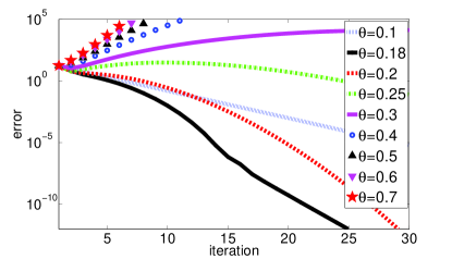
We discretize (55) using standard centered finite differences in space and backward Euler in time on a grid with $\Delta x=2\times 10^{-2}$ and $\Delta t=4\times 10^{-3}$. For the DNWR method, we consider two cases: first, we choose $a=3$ and $b=2$, i.e., we split the spatial domain $\Omega:=(-3,2)$ into two non-overlapping subdomains $\Omega_{1}=(-3,0)$ and $\Omega_{2}=(0,2)$, see Figure 1. This is the case of DNWR when the Dirichlet subdomain is larger than the Neumann subdomain ($a>b$), corresponding to Theorem 2. For the second case, we take $a=2$ and $b=3$, so that the Dirichlet domain is smaller than the Neumann one, as in Theorem 3. We test the algorithm by choosing $h^{0}(t)=t^{2},t\in[0,T]$ as an initial guess. Figures 3 and 4

Fig. 3: Convergence of DNWR for $a>b$ using various relaxation parameters $\theta$ for $T=2$, on the left for $\kappa(x)=1$ and on the right for $\kappa(x)=1+e^{x}$

Fig. 4: Convergence of DNWR for $a<b$ using various relaxation parameters $\theta$ for $T=2$, on the left for $\kappa(x)=1$ and on the right for $\kappa(x)=1+e^{x}$

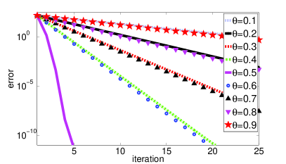
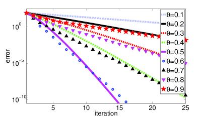
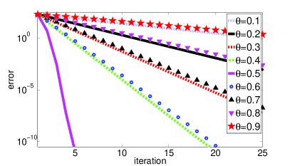
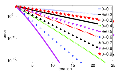
give the convergence curves for $T=2$ and for different values of the parameter $\theta$ for $\kappa(x)=1$ on the left, and $\kappa(x)=1+e^{x}$ on the right. We see that for a small time window, we get linear convergence for all relaxation parameters $\theta$, except for $\theta=1/2$, when we observe superlinear convergence.

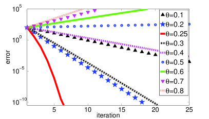
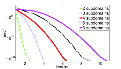
Next, we show an experiment for the NNWR algorithm in the spatial domain $\Omega=(0,6)$, with the same discretization parameters $\Delta x$ and $\Delta t$ as above, and for the time window $T=2$. Now onward we always use $\kappa(x)=1$, unless otherwise specified. In Figure 5, we consider a decomposition into two to six unequal subdomains, whose widths are shown in Table 1. On the left panel, we show the convergence in the four-subdomain case as a function of the relaxation parameter $\theta$, whereas on the right panel, we show the convergence for $\theta=1/4$ as we vary the number of subdomains. We observe superlinear convergence for $\theta=1/4$, and only linear convergence for the other choices, and also that convergence slows down as the number of subdomains is increased, as expected.

Table 1: Subdomain lengths used for the NNWR experiments in Fig.5.

No. of subdomains	$h_{1}$	$h_{2}$	$h_{3}$	$h_{4}$	$h_{5}$	$h_{6}$
2	3.50	2.50
3	2.30	2.30	1.40
4	1.20	2.40	1.80	0.60
5	1.80	1.40	1.08	1.00	0.72
6	1.20	0.80	1.00	1.20	1.00	0.80

Fig. 5: Convergence of NNWR with four subdomains and various relaxation parameters on the left, and dependence of NNWR on the number of subdomains for $\theta=1/4$ on the right

Fig. 6: Comparison of the numerically measured convergence rates and the theoretical error estimates for DNWR for $\kappa(x)=1$ with $T=2$ on the left, and $T=50$ on the right

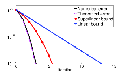
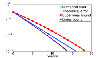
We now compare the numerical behavior of DNWR and NNWR with our theoretical estimates in Sections 2 and 3. In Figure 6, we show for the DNWR algorithm a comparison between the numerically measured convergence for the discretized problem, the theoretical convergence for the continuous model problem (calculated using inverse Laplace transforms), and the linear and superlinear convergence estimates shown in Theorem 2, for $a=3$, $b=2$, $\kappa(x)=1$. We see that for a short time interval, $T=2$, the algorithm converges superlinearly, and the superlinear bound is quite accurate. For the long time interval $T=50$, the algorithm converges linearly, and the linear convergence estimate is now more accurate.

Fig. 7: Comparison of the numerically measured convergence rates and the theoretical error estimates for NNWR for $\kappa(x)=1$ with $\theta=1/4$ and $T=2$, on the left for two subdomains, and on the right for many subdomains

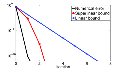
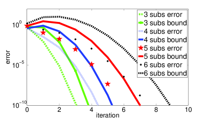
Similarly, we show in Figure 7 a comparison of the numerically measured convergence for the NNWR algorithm for $\theta=1/4$ and $\kappa(x)=1$, and the theoretical estimates from Theorem 5. On the left, we show the results for the two subdomain case (subdomain lengths are as in the first line of Table 1), where we also plotted the linear estimate from [16], and on the right, we show the results for the case of many subdomains of equal length for $\Omega=(0,6)$.

We now compare in Figure 8

Fig. 8: Comparison of DNWR and NNWR with Schwarz waveform relaxation

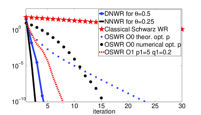
the performance of the DNWR and NNWR algorithms for two subdomains with the Schwarz Waveform Relaxation algorithms from [11, 2] with overlap. We use an overlap of length $2\Delta x$, where $\Delta x=1/50$. We observe that the DNWR and NNWR algorithms converge faster than the overlapping Schwarz WR iteration. Only a higher order optimized Schwarz waveform relaxation algorithm comes close to the performance of the DNWR algorithm in this experiment.

We show an experiment for the NNWR algorithm in two dimension for the following model problem

$$\partial_{t}u-\left(\partial_{xx}u+\partial_{yy}u\right)=0,u(x,y,0)=\sin(2\pi x)\sin(3\pi y).$$

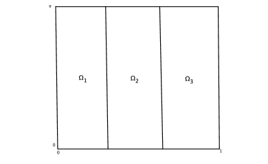
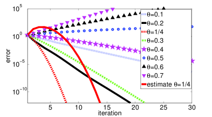
We decompose our domain $\Omega:=(0,1)\times(0,\pi)$ into three non-overlapping subdomains $\Omega_{1}=(0,2/5)\times(0,\pi)$, $\Omega_{2}=(2/5,3/4)\times(0,\pi)$, $\Omega_{3}=(3/4,1)\times(0,\pi)$, see Figure 9 on the left. On the right, we plot the numerical errors of the NNWR algorithm for various $\theta$ and the theoretical estimates from Theorem 11 for $\theta=1/4$ and again observe superlinear convergence.

Fig. 9: Decomposition of 2d domain into strips on the left, and convergence of NNWR using various relaxation parameters $\theta$ for $T=0.2$ on the right

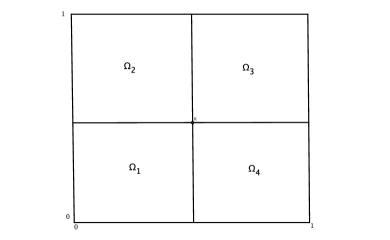
We conclude this section with a numerical experiment not covered by our analysis: we decompose the two dimensional domain $\Omega:=(0,1)\times(0,1)$ into four non-overlapping subdomains $\Omega_{1}=(0,1/2)\times(0,1/2)$, $\Omega_{2}=(0,1/2)\times(1/2,1)$, $\Omega_{3}=(1/2,1)\times(1/2,1)$, $\Omega_{4}=(1/2,1)\times(0,1/2)$, such that a cross point is present, see Figure 10 on the left. On the right, we show that the convergence of the NNWR algorithm is again superlinear.

Fig. 10: Decomposition of 2d domain with a crosspoint on the left, and convergence of NNWR using various relaxation parameters $\theta$ for $T=0.2$ on the right

8 Conclusions

We introduced two new classes of space-time parallel algorithms, the Dirichlet-Neumann waveform relaxation (DNWR) and the Neumann-Neumann waveform relaxation (NNWR) algorithms. For the one-dimensional heat equation, we proved superlinear convergence for both algorithms for a particular choice of the relaxation parameter. For the NNWR, our convergence estimate holds for a decomposition into many subdomains, and we also gave an extension to two spatial dimensions. We are currently working on the generalization of our analysis for the DNWR algorithm to the case of many subdomains and higher spatial dimensions, and we are also studying the convergence for $\theta\neq 1/2$ in more detail.

References

- [1] A. Bellen and M. Zennaro, The use of Runge-Kutta formulae in waveform relaxation methods, Appl. Numer. Math., (1993).
- [2] D. Bennequin, M. J. Gander, and L. Halpern, A Homographic Best Approximation Problem with Application to Optimized Schwarz Waveform Relaxation, Math. of Comp., (2009), pp. 185–223.
- [3] M. Bjørhus, A note on the convergence of discretized dynamic iteration, BIT, (1995), pp. 291–296.
- [4] Petter E. Bjørstad and O. B. Widlund, Iterative Methods for the Solution of Elliptic Problems on Regions Partitioned into Substructures, SIAM J. Numer. Anal., (1986).
- [5] J. F. Bourgat, R. Glowinski, P. L. Tallec, and M. Vidrascu, Variational Formulation and Algorithm for Trace Operator in Domain Decomposition Calculations, in Domain Decomposition Methods, T. F. Chan, R. Glowinski, J. Périaux, and O. B. Widlund, eds., SIAM, 1989, pp. 3–16.
- [6] J. H. Bramble, J. E. Pasciak, and A. H. Schatz, An Iterative Method for Elliptic Problems on Regions Partitioned into Substructures, Mathematics of Computation, (1986).
- [7] J. R. Cannon, The One-Dimensional Heat Equation, Addison-Wesley Publishing Company, 1984.
- [8] R. V. Churchill, Operational Mathematics, McGraw-Hill, 2nd ed., 1958.
- [9] M. J. Gander, Optimized Schwarz methods, SIAM J. Numer. Anal., 44 (2006), pp. 699–732.
- [10] M. J. Gander and L. Halpern, Absorbing Boundary Conditions for the Wave Equation and Parallel Computing, Math. of Comput., 74 (2004), pp. 153–176.
- [11] , Optimized Schwarz Waveform Relaxation for Advection Reaction Diffusion Problems, SIAM J. Num. Anal., 45 (2007), pp. 666–697.
- [12] M. J. Gander, L. Halpern, and F. Nataf, Optimal Schwarz Waveform Relaxation for the One Dimensional Wave Equation, SIAM J. Num. Anal., 41 (2003), pp. 1643–1681.
- [13] M. J. Gander and A. M. Stuart, Space-time continuous analysis of waveform relaxation for the heat equation, SIAM J. for Sci. Comput., 19 (1998), pp. 2014–2031.
- [14] E. Giladi and H. Keller, Space time domain decomposition for parabolic problems, Tech. Report 97-4, Center for research on parallel computation CRPC, Caltech, 1997.
- [15] R. Jeltsch and B. Pohl, Waveform relaxation with overlapping splittings, SIAM J. Sci. Comput., (1995).
- [16] F. Kwok, Neumann-Neumann Waveform Relaxation for the Time-Dependent Heat Equation, submitted in 21st International Conference on Domain Decomposition Methods for PDEs.
- [17] E. Lelarasmee, A. Ruehli, and A. Sangiovanni-Vincentelli, The waveform relaxation method for time-domain analysis of large scale integrated circuits, IEEE Trans. Compt.-Aided Design Integr. Circuits Syst., 1 (1982), pp. 131–145.
- [18] E. Lindelöf, Sur l’application des méthodes d’approximations successives à l’étude des intégrales réelles des équations différentielles ordinaires, Journal de Mathématiques Pures et Appliquées, (1894).
- [19] P. L. Lions, On the Schwarz alternating method, in First International Symposium on Domain Decomposition Methods for PDEs, I, (1989).
- [20] B. C. Mandal, A Time-Dependent Dirichlet-Neumann Method for the Heat Equation, submitted in 21st International Conference on Domain Decomposition Methods for PDEs.
- [21] L. Martini and A. Quarteroni, An Iterative Procedure for Domain Decomposition Methods: a Finite Element Approach, SIAM, in Domain Decomposition Methods for PDEs, I, (1988), pp. 129–143.
- [22] , A Relaxation Procedure for Domain Decomposition Method using Finite Elements, Numer. Math., (1989).
- [23] U. Miekkala and O. Nevanlinna, Convergence of dynamic iteration methods for initial value problems, SIAM J. Sci. Stat. Comput., (1987).
- [24] O. Nevanlinna, Remarks on Picard-Lindelöf iterations part i. BIT, 1989.
- [25] , Remarks on Picard-Lindelöf iterations part ii. BIT, 1989.
- [26] Fritz Oberhettinger and L. Badii, Tables of Laplace Transforms, Springer-Verlag, 1973.
- [27] E. Picard, Sur l’application des méthodes d’approximations successives à l’étude de certaines équations différentielles ordinaires, Journal de Mathématiques Pures et Appliquées, (1893).
- [28] A. Quarteroni and A. Valli, Domain Decomposition Mathods for Partial Differential Equations, Clarendon Press, 1999.
- [29] Y. D. Roeck and P. L. Tallec, Analysis and Test of a local domain decomposition preconditioner, in Domain Decomposition Methods for PDEs, I, R. Glowinski et al., ed., Philadelphia, 1991, SIAM, pp. 112–128.
- [30] J. L. Schiff, The Laplace Transform, Springer, 1991.
- [31] P. L. Tallec, Y. D. Roeck, and M. Vidrascu, Domain decomposition methods for large linearly elliptic three-dimensional problems, J. of Comput. and App. Math., (1991).
- [32] A. Toselli and O. B. Widlund, Domain Decomposition Methods, Algorithms and Theory, Springer, 2005.