Spin-spin interaction in the bulk of topological insulators

Abstract

We apply mean-field theory and Hirsch-Fye quantum Monte Carlo method to study the spin-spin interaction in the bulk of three-dimensional topological insulators. We find that the spin-spin interaction has three different components: the longitudinal, the transverse and the transverse Dzyaloshinskii-Moriya-like terms. When the Fermi energy is located in the bulk gap of topological insulators, the spin-spin interaction decays exponentially due to Bloembergen-Rowland interaction. The longitudinal correlation is antiferromagnetic and the transverse correlations are ferromagnetic. When the chemical potential is in the conduction or valence band, the spin-spin interaction follows power law decay, and isotropic ferromagnetic interaction dominates in short separation limit.

I Introduction

Time-reversal invariant topological insulatorsFu et al. (2007); Xia et al. (2009); Zhang et al. (2009); Moore (2010); Hasan and Kane (2010); Qi and Zhang (2011) (TIs) have attracted much attention and have been extensively investigated in the past few years. Three-dimensional (3D) TIs are fully gapped in the bulk with strong spin-orbit coupling, but have protected gapless surface states. Semiconducting thermoelectric Bi₂Se₃, Bi₂Te₃ and Sb₂Te₃ are most studied promising materials of TIs with large bulk band gaps $\sim$ 0.3eV and gapless Dirac fermions (quasi-particles) on the surface .Zhang et al. (2009); Hasan and Kane (2010); Qi and Zhang (2011) There are many interesting phenomena related to spin-orbit locked TI surface statesQi et al. (2008), including the topological magnetoelectric effectQi et al. (2008), the half integer quantum Hall effect Nomura and Nagaosa (2011), the image magnetic monopole Qi et al. (2009); Zang and Nagaosa (2010) induced by electric charge near the TI surface state, the topologically quantized magneto-optical Kerr and Faraday rotation Tse and MacDonald (2010, 2011) in units of the fine structure constant Maciejko et al. (2010); Lan et al. (2011) and the repulsive Casimir effect between TIs with opposite topological magnetoelectric polarizabilities Grushin and Cortijo (2011); Grushin et al. (2011); Chen and Wan (2011), etc..

To study the various phenomena mentioned above and control the transport properties of TIs, one needs to break the time-reversal symmetry and generate an energy gap for TI surface Dirac fermions. Surface- and bulk-doping with magnetic impurities are feasible methods. Chen et al. (2010); Wray et al. (2011); Okada et al. (2011); Valla et al. (2012); Hor et al. (2010); Scholz et al. (2012) There are numerous works demonstrating that magnetic doping can induce a surface band gap.Chen et al. (2010); Wray et al. (2011); Okada et al. (2011) However, some other experiments could not observe the gap opened by magnetic doping Valla et al. (2012); Hor et al. (2010); Scholz et al. (2012), such that the Ruderman-Kittel-Kasuya-Yosida (RKKY)Kasuya (1956); Ruderman and Kittel (1954); Yosida (1957) interactions between magnetic impurities have attracted much attention. For the surface-doping Liu et al. (2009), careful theoretical investigations Zhu et al. (2011); Abanin and Pesin (2011); Biswas and Balatsky (2010) show that the RKKY interactions mediated by surface Dirac fermions are much complicated than expected. Other than the normal Heisenberg-like interactions, there may exist Ising-like and Dzyaloshinskii-Moriya (DM)-like interactions between magnetic impurities on the surface of TIs. For the bulk-doping Lü et al. (2013), mean-field analysis Rosenberg and Franz (2012) shows that there may exist ferromagnetic (FM) or antiferromagnetic (AFM) correlation between magnetic impurities. Density functional theory calculationsSchmidt et al. (2011); Henk et al. (2012); Zhang et al. (2012) demonstrate complicated anisotropic spin texture in magnetically doped TIs. However, the importance of spin-orbit coupling in RKKY interactions has not been clarified. A recent experimentKim et al. (2013) sheds light on complicated RKKY interactions in the bulk of TIs. It is reported that magnetic impurities in the bulk of Fe_xBi₂Se₃ behave like ferromagnetic-cluster glass for $x\sim 0.025$, and valence-bond glass for the region from $x\sim 0.03$ up to $x\sim 0.1$. A detailed analysis on the spin-spin interaction in the bulk of TIs may provide clue to these results.

In this paper, we apply mean-field theory and Hirsch-Fye quantum Monte Carlo (HFQMC) Hirsch and Fye (1986) method to study the carrier-mediated spin-spin interaction between two magnetic impurities in the bulk of TIs. To get a heuristic physical picture about the correlation between magnetic impurities, we use mean field theory to study the problem before applying the quantum Monte Carlo method. We take two steps. Firstly, we use the self-consistent Hartree-Fork approximation to estimate the local moment of a single impurity. The self-consistent Hartree-Fork approximation gives analytical criterionAnderson (1961) about the formation of local moment in the background of electron gas. It was also applied to study the local moment problem in other systems (i.e. semiconductorHaldane and Anderson (1976) and grapheneUchoa et al. (2008)). Once we get a nonzero magnetic moment, we use functional integralNegele and Orland (1998) approach to study the interaction between magnetic impurities, the approach is a little different from the original RKKY perturbation theory because we have to deal with spin-orbit coupled systems. When quantum fluctuation is significant, the mean-field results are suspectable, so furthermore, we use the quantum Monte Carlo method to study the problem. The HFQMC technique is a numerically exact method, it is widely used to study the magnetic properties of impurities in metals, i.e. the local moment of impurityHirsch and Fye (1986); Fye and Hirsch (1988), the Kondo effectFye et al. (1987) and the interaction between localized moments Fye et al. (1987); Hirsch and Lin (1987), etc.. Recently, the HFQMC technique is applied to study the magnetic properties of Anderson impurities in dilute magnetic semiconductorsBulut et al. (2007) and grapheneHu et al. (2011).

The paper is organized as follows. We present the model and mean-field results in Sec. II. In Subsection II.1, we introduce the model Hamiltonian describing the magnetic impurities in TIs. In subsection II.2, we present the mean-field approach and analyze the spin-spin interaction for different chemical potential regions and impurity energy levels. In Sec. III, we show the results obtained by the HFQMC simulations. We investigate the local moment in subsection III.1, and the spin-spin interaction in subsection III.2. Finally, discussions and conclusions are given in Sec. IV.

II Model Hamiltonian and mean field results

II.1 Model Hamiltonian

We use the four-band modelLü et al. (2013); Lu et al. (2010); Shan et al. (2010); Shen et al. (2011) to describe the bulk states of TIs. The coupling between magnetic impurities and bulk states can be described by the Anderson modelHewson (1997). The total Hamiltonian with TI host material, magnetic impurities and hybridization between TI bulk states and impurities can be written as

$$\mathcal{H} = \mathcal{H}_{\text{b}}+\mathcal{H}_{d}+\mathcal{H}_{\text{hb}},$$ (1)

$$\mathcal{H}_{\text{b}} = \int{\mathbf{d}r}\,\Psi^{\dagger}\left[(m-B{v_{F}^{2}}\bm{k}^{2})\tau_{z}+v_{F}{\bm{k}\cdot\sigma}\tau_{x}-\mu\right]\Psi,$$ (2)

$$\mathcal{H}_{d} = \sum_{j=1,2;s=\uparrow,\downarrow}d_{j,s}^{\dagger}\left(\epsilon_{d}-\mu\right)d_{j,s}+U{}d_{j,\uparrow}^{\dagger}d_{j,\uparrow}d_{j,\downarrow}^{\dagger}d_{j,\downarrow},$$ (3)

$$\mathcal{H}_{\text{hb}} = \int{\mathbf{d}}r\,\sum_{j=1,2}{d^{\dagger}_{j}}V_{j}(\bm{r})\Psi(\bm{r})+h.c.,$$ (4)

where $\bm{k}=-i\nabla$ is the momentum operator (we take the Planck constant $\hbar=1$), $\tau_{z,x}$ and $\sigma_{x,y,z}$ are the Pauli matrices for different orbits and different spins, respectively. $v_{F}$ is the velocity of the bulk Dirac fermions, and $(m-B{v_{F}^{2}}\bm{k}^{2})$ is the effective mass which can be derived from the $k\cdot{p}$ theoryZhang et al. (2009). The sign of $mB$ determines the topology of the bulk states: $mB>0$ ($mB<0$) corresponds to a topological (normal) insulator. $\mu$ is the chemical potential which can be tuned by doping Hsieh et al. (2009). The basis vectors of the TI bulk states are chosen as

$$\Psi=\left(\begin{array}[]{cccc}\psi_{a\uparrow}&\psi_{a\downarrow}&\psi_{b\uparrow}&\psi_{b\downarrow}\end{array}\right)^{T},$$

where $a$ and $b$ are orbit indices. $d^{\dagger}_{j\uparrow(\downarrow)}$ and $d_{j\uparrow(\downarrow)}$ are creation and annihilation operators of spin-up (spin-down) state on the $j$-th impurity site. $(\epsilon_{d}-\mu)$ is the impurity energy level and $U$ is the on-site Coulomb interaction. $V_{j}(\bm{r})$ is a $2\times 4$ hybridization matrix, which can be written in the following form in short range coupling limit,

$$V_{j}(\bm{r})=\left(\begin{array}[]{cccc}V_{a}&0&V_{b}&0\\ 0&V_{a}&0&V_{b}\\ \end{array}\right)\delta(\bm{r}-\bm{r}_{j}),$$

where $\bm{r}_{j}$ is the coordinate of the $j$-th impurity. Furthermore, we consider the case that the impurities are symmetrically coupled with the two orbits, i.e. $V_{a}=V_{b}=V_{0}$. Without loss of generality, we assume that the two impurities are put on the $y$-axis and the distance is $R$. Fig. (1) gives a schematic of our model.

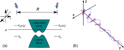
Figure 1: (a) Schematic of two magnetic impurities in the bulk of TIs, with RKKY interaction mediated by the bulk states of TIs. The two impurities are put on the y-axis, $R$ is the distance between impurities. $\epsilon_{d}$ and $\epsilon_{d}+U$ are energy levels of impurities, the conduction and valence band indicate the band structure of TIs. The chemical potential $\mu$ can be tuned into the valence band, conduction band or in the bulk gap by doping. (b) Illustration of spin-spin interaction as a function of distance $R$. The blue line means the correlation strength and arrows denote the rotation of spin-spin interaction due to the spin-orbit coupling in TIs.

II.2 Mean-field results

Before a detailed discussion on the spin-spin interaction, we first make a note on the units and parameters chosen in this paper. The Planck constant $\hbar$ is set to be 1, and we choose the parameter $m$ of TIs as energy unit. In the continuous limit, the summation over momentum is approximated by integration, $\frac{1}{N_{0}}\sum_{k}\rightarrow\frac{6\pi^{2}}{k_{T}^{3}}\int\frac{\mathbf{d}^{3}k}{(2\pi)^{3}}$, where $N_{0}$ is the number of system sites with $k_{T}$ being the truncation of momentum, which is determined by the cut-off of the band width $D=\sqrt{({v_{F}}{k_{T}})^{2}+(m-B{v_{F}^{2}}{k_{T}^{2}})^{2}}$. $\Gamma_{0}=\pi\rho_{0}{V_{0}^{2}}$ represents the hybridization strength among the impurities and the bulk states, where $\rho_{0}=N_{0}/2D$ is the density of states per spin at the chemical potential. $D=30m$ and $\Gamma_{0}=0.5$ are chosen in numerical calculationsLü et al. (2013).

In order to investigate the spin-spin interaction between the two magnetic impurities, a proper parameter region (the on-site Coulomb repulsion $U$, the impurity energy level $\epsilon_{d}$ and the chemical potential $\mu$) are required for the well developed local moment. Under the self-consistent Hartree-Fork approximation, the imaginary-time Green’s function of spin-up and spin-down electrons are

$$g_{\uparrow}(\tau)=\frac{1}{\beta}\sum_{i\omega_{n}}\frac{e^{-i\omega_{n}\tau}}{i\omega_{n}-[\epsilon_{d}-\mu+\Sigma_{1}(i\omega_{n})+U\langle{n_{\downarrow}}\rangle]},$$ (5)

$$g_{\downarrow}(\tau)=\frac{1}{\beta}\sum_{i\omega_{n}}\frac{e^{-i\omega_{n}\tau}}{i\omega_{n}-[\epsilon_{d}-\mu+\Sigma_{1}(i\omega_{n})+U\langle{n_{\uparrow}}\rangle]},$$ (6)

where $\beta=1/k_{B}T$, $T$ is the temperature and $k_{B}$ is the Boltzmann constant. $\Sigma_{1}(i\omega_{n})$ is the self-energy comes from the hybridization between the impurity and the bulk states, the exact form of the self-energy is

$$\Sigma_{1}(i\omega_{n})=-\frac{12i{}D\Gamma_{0}}{k_{T}^{3}}\frac{\sqrt{2mB-\lambda-1}-\sqrt{2mB+\lambda-1}}{2\sqrt{2}mB\lambda},$$ (7)

$$\lambda=\sqrt{1+4mB(mB(i\omega_{n}+\mu)^{2}-1)},$$ (8)

$\langle{n_{\downarrow}}\rangle$ and $\langle{n_{\uparrow}}\rangle$ are expectation values of local spin-up and spin-down states, which can be solved by self-consistent equations

$$\langle{n_{\downarrow}}\rangle=g_{\downarrow}(\tau\rightarrow 0^{-}),$$ (9)

$$\langle{n_{\uparrow}}\rangle=g_{\uparrow}(\tau\rightarrow 0^{-}).$$ (10)

Fig. (2) and Fig. (3) show the numerical results of local moment as a function of Hubbard $U$, impurity energy level $\epsilon_{d}-\mu$ and chemical potential $\mu$. One can find that the local moment $m_{d}>0.72$ when $\epsilon_{d}-\mu=-1.5$, $U=3.0$, and $k_{B}T=1/16$. Therefore, within the self-consistent mean-field approximation, $U\geq 3.0$ is sufficiently large to generate a non-zero local moment if $\epsilon_{d}-\mu=-1.5$ and $k_{B}T\leq 1/16$.

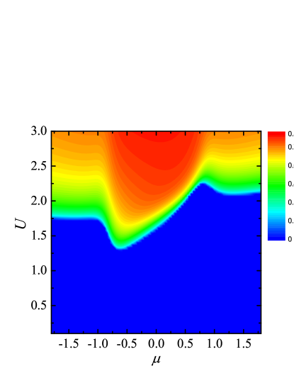
Figure 2: Mean field results of single impurity local moment ${m_{d}}=\langle{n_{\uparrow}}\rangle-\langle{n_{\downarrow}}\rangle$ as a function of chemical potential $\mu$ and Hubbard $U$. Impurity energy level $\epsilon_{d}-\mu=-1.5$ and temperature $k_{B}T=1/16$ were chosen in the calculation.

Now we construct the spin-spin interaction between the local moments, the partition function of the two impurities in the bulk of TIs can be written as

$${\cal Z}=\int{{\cal D}d^{\dagger}{\cal D}d}\mathrm{e}^{-\mathcal{S}},$$ (11)

$$\mathcal{S}=-\int_{0}^{\beta}{\mathrm{d}}\tau{}d^{\dagger}\left[\frac{\partial}{\partial{\tau}}+\left(\epsilon_{d}-\mu+U{}n_{d}+\Sigma_{1}\right.\right.$$

$$\left.\left.-U\frac{m_{d}}{2}{\cal U}\sigma_{z}{\cal U}^{\dagger}\right)+(\Sigma_{2}\lambda_{x}+\Sigma_{3}\lambda_{y}\sigma_{y})\right]d,$$ (12)

where $n_{d}=\langle{n_{\uparrow}}\rangle+\langle{n_{\downarrow}}\rangle$ is the local charge, $m_{d}$ is the local moment, $\lambda_{x}$ and $\lambda_{y}$ are the Pauli matrices in the space of two impurities, $\Sigma_{2}$ and $\Sigma_{3}$ are self-energy from hybridization between impurity states and bulk electrons, the exact form of $\Sigma_{2}$ and $\Sigma_{3}$ are given by

$$\Sigma_{2}(i\omega_{n})=\frac{12D\Gamma_{0}}{\pi{R}{k_{T}^{3}}}\int_{0}^{k_{T}}{\mathrm{d}}k\frac{k(i\omega_{n}+\mu){\sin(kR)}}{(i\omega_{n}+\mu)^{2}-E_{\bm{k}}^{2}},$$ (13)

$$\Sigma_{3}(i\omega_{n})=\frac{12D\Gamma_{0}}{\pi{R^{2}}{k_{T}^{3}}}\int_{0}^{k_{T}}{\mathrm{d}}k\frac{k[{\sin(kR)-kR\cos(kR)}]}{(i\omega_{n}+\mu)^{2}-E_{\bm{k}}^{2}},$$ (14)

$$E_{\bm{k}}^{2}=k^{2}+(1-mBk^{2})^{2}.$$ (15)

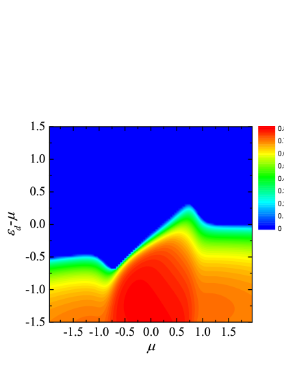
Figure 3: Mean field results of single impurity local moment ${m_{d}}=\langle{n_{\uparrow}}\rangle-\langle{n_{\downarrow}}\rangle$ as a function of chemical potential $\mu$ and impurity energy level $\epsilon_{d}-\mu=-1.5$, Hubbard $U=3.0$ and temperature $k_{B}T=1/16$ were chosen in numerical calculation.

$\Sigma_{2}$ represents the normal propagation of electrons in the bulk of TIs, while $\Sigma_{3}$ represents the spin-flipping propagation of electrons in the bulk of TIs due to spin-orbit coupling. In Eq. (12), we introduce a SU(2) matrix $\mathcal{U}$ to describe the spin degrees of freedom of the impurity with non-vanishing local moment. $\mathcal{U}$ can be parameterized in the following form,

$${\cal U}=\left(\begin{array}[]{cc}b_{1}&b_{2}^{\dagger}\\ -b_{2}&b_{1}^{\dagger}\\ \end{array}\right),$$ (16)

with SU(2) constraint on the bosonic creation and annihilation operators $b^{\dagger}_{1,2}$, $b_{1,2}$:

$$b_{1}^{\dagger}b_{1}+b_{2}^{\dagger}b_{2}=1.$$ (17)

Local moment $m_{d}$ is defined as $m_{d}=\langle{f_{\uparrow}^{\dagger}f_{\uparrow}}\rangle-\langle{f_{\downarrow}^{\dagger}f_{\downarrow}}\rangle$ and $f=\mathcal{U}^{\dagger}d$. Under the parametrization (16) and up to the self-consistent Hartree-Fork approximation, we find that the local spin can be expressed as

$$S^{z}=d_{\uparrow}^{\dagger}{d_{\uparrow}}-d_{\downarrow}^{\dagger}{d_{\downarrow}}=m_{d}\left(b_{1}^{\dagger}{b_{1}}-b_{2}^{\dagger}{b_{2}}\right),$$ (18)

$$S^{x}=d_{\uparrow}^{\dagger}{d_{\downarrow}}+d_{\downarrow}^{\dagger}{d_{\uparrow}}=m_{d}\left(b_{1}^{\dagger}{b_{2}}+b_{2}^{\dagger}{b_{1}}\right),$$ (19)

$$S^{y}=-i\left(d_{\uparrow}^{\dagger}{d_{\downarrow}}-d_{\downarrow}^{\dagger}{d_{\uparrow}}\right)=-i{}m_{d}\left(b_{1}^{\dagger}{b_{2}}-b_{2}^{\dagger}{b_{1}}\right).$$ (20)

One can find that Eq. (18)-(20) tend to the Schwinger-Wigner representationTsvelik (2007) of spin when $m_{d}\rightarrow 1$. In the loop approximation, we find that the spin-spin interaction between the two magnetic impurities can be written as

$$H_{RKKY}={\cal K}\bm{S}_{1}{\cdot}\bm{S}_{2}+{\cal Q}\left(S_{1}^{\parallel}S_{2}^{\parallel}-\bm{S}_{1}^{\perp}{\cdot}\bm{S}_{2}^{\perp}\right)+{\cal R}\left(\bm{S}_{1}{\times}\bm{S}_{2}\right)_{\parallel},$$ (21)

where $\parallel$ ($\perp$) means the component(s) parallel (perpendicular) to the y-axis. The range functions are given by

$${\cal K}(R,\mu)=2J^{2}\frac{1}{\beta}\sum_{i\omega_{n}}\left[{\Sigma_{2}^{2}(i\omega_{n})}\right],$$ (22)

$${\cal Q}(R,\mu)=2J^{2}\frac{1}{\beta}\sum_{i\omega_{n}}\left[{\Sigma_{3}^{2}(i\omega_{n})}\right],$$ (23)

$${\cal R}(R,\mu)=2J^{2}\frac{1}{\beta}\sum_{i\omega_{n}}\left[2{\Sigma_{2}(i\omega_{n})\Sigma_{3}(i\omega_{n})}\right],$$ (24)

and $J=U/(\epsilon_{d}-\mu+n_{d}U)^{2}$. The prefactor 2 indicates that there are two orbits in the bulk of TIs. One can find that the spin-spin interaction between magnetic impurities in the bulk of TI is similar to the RKKY interaction between magnetic impurities on TI surfaceZhu et al. (2011). There are three different terms, an isotropic Heisenberg-like term, an anisotropic term and a DM-like term. The difference is that the anisotropic term is not an Ising-like term but a XXZ-model-like term.

Now we analyze the range functions in more details. It is difficult to get analytical expressions due to the complex band structure of TIs, here we present the numerical results for three typical cases: (1) the chemical potential is in the gap of TIs, $-1<\mu<1$, (2) the chemical potential is in the conduction band, $\mu>1$, and (3) the chemical potential is in the valance band, $\mu<-1$.

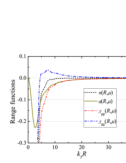
Figure 4: Range functions of RKKY interaction between two magnetic impurities as a function of distance $k_{T}R$ when chemical potential $\mu=0$. $\mathcal{J}_{yy}=\mathcal{K}(R,\mu)+\mathcal{Q}(R,\mu)$ is the longitudinal spin-spin interaction, $\mathcal{J}_{zz}=\mathcal{K}(R,\mu)-\mathcal{Q}(R,\mu)$ is the transverse spin-spin interaction. Local moment $m_{d}=1$ and zero-temperature limit were taken in the calculation.

Figure 5: Range functions of RKKY interaction between two magnetic impurities as a function of distance $k_{T}R$ when chemical potential $\mu=2$. $\mathcal{J}_{yy}=\mathcal{K}(R,\mu)+\mathcal{Q}(R,\mu)$, $\mathcal{J}_{zz}=\mathcal{K}(R,\mu)-\mathcal{Q}(R,\mu)$ and $\mathcal{J}_{xz}=\mathcal{R}(R,\mu)$. Local moment $m_{d}=1$ and zero-temperature limit were taken in the calculation.

Figure 6: Product $\mathcal{K}(R,\mu){(k_{T}R)}^{3}$, $\mathcal{Q}(R,\mu){(k_{T}R)}^{3}$ and $\mathcal{R}(R,\mu){(k_{T}R)}^{3}$ as functions of dimensionless distance $k_{T}R$. $\mu=2$, $m_{d}=1$ and $T=0$ were chosen in numerical calculation.

For the first case, we find that the DM-like term $\mathcal{R}(R,\mu)$ equals to zero spontaneously, and the other two terms decay exponentially with respect to $k_{T}R$ due to the BR interaction mediated by massive Dirac electrons in the bulk of TIs. In the short distance limit $R\rightarrow 0$, the isotropic spin-spin interaction dominates, $\mathcal{K}(0,\mu)<0$, and the anisotropic spin-spin interaction tends to vanish, $\mathcal{Q}(0,\mu)=0$. In the long distance limit, we find that the anisotropic spin-spin interaction $\mathcal{Q}(R,\mu)$ dominates and the isotropic spin-spin interaction $\mathcal{K}(R,\mu)$ decays more rapidly (one can see in Fig. (4) that $\mathcal{J}_{yy}(R,\mu)=-\mathcal{J}_{zz}(R,\mu)$ in the long distance limit,i.e. $k_{T}R>10$). All of these phenomena are related to spin-orbit coupling in TIs. When spin-orbit coupling tends to zero, the self-energy $\Sigma_{3}\rightarrow 0$ and $\mathcal{Q}(R,\mu)\rightarrow 0$. A typical example is the short distance limit. One can check in Eq. (14) that $\Sigma_{3}\rightarrow 0$ while $R\rightarrow 0$. The long distance limit is more interesting because it reflects the special band structure of TIs. As shown in Fig. (1), the minimal gap is not located at $\bm{k}=0$, so that the decay length of spin-orbit coupled states are larger than that of uncoupled states, and $\mathcal{K}(R,\mu)$ decays much more rapidly than $\mathcal{Q}(R,\mu)$. Therefore, when the chemical potential is tuned into the gap of TIs, the diluted magnetic impurities prefer paramagnetic phase not only because the effective interactions decay exponentially but also because of the anisotropic spin-spin interaction dominates.

For the second and third cases, we find that $\mathcal{K}(R,\mu)=\mathcal{K}(R,-\mu)$, $\mathcal{Q}(R,\mu)=\mathcal{Q}(R,-\mu)$ and $\mathcal{R}(R,\mu)=-\mathcal{R}(R,-\mu)$. Shown in Fig. (5) are the range functions for $\mu=2.0$. In the short distance limit $R\rightarrow 0$, we also find that $\mathcal{Q}(R,\mu)=\mathcal{R}(R,\mu)=0$ and $\mathcal{K}(R,\mu)<0$. In short separation range $0<k_{T}R<20$, the oscillation and decay are very complex due to the complex band structure of TIs. In the large separation limit $R\rightarrow\infty$, the oscillation and decay are determined by bulk states near the Fermi surface and as shown in Fig. (6), all of the three range functions decay with power law $\sim\cos{(2k_{F}R)/R^{3}}$, which is the same as in the conventional 3D electron gas. There are two interesting things in Fig (6). Firstly, similar to the surface doping Zhu et al. (2011), one can see in Fig. (6) that the red (long-dashed) line and black (solid) line are almost of opposite sign, and the maxima and minima of blue (short-dashed) line always appear at the zero points of red and black lines (i.e. $k_{T}R=60$), where the Heisenberg-like term and XXZ-model-like term vanish and DM term dominates. Secondly, the oscillation center of $\mathcal{R}(R,\mu)(k_{T}R)^{3}$ does not locate at zero, which indicates that there is a remainder spin-rotation behind the oscillation.

In addition, we want to clarify that the range functions presented above tend to the conventional RKKY interaction in the 3D electron gas in the following limits: spin-orbit coupling $\rightarrow 0$ and $\mu\gg 1$. One can check that $\Sigma_{3}\rightarrow 0$ when spin-orbit coupling $\rightarrow 0$, so that $\mathcal{Q}(R,\mu)=\mathcal{R}(R,\mu)=0$. While $\mu\gg 1$, the dispersion relation (15) can be approximated by $E_{\bm{k}}=\bm{k}^{2}/2M$ with $2M=1/mB$. We carry out the integration over momentum and frequency in Eq. (13) and Eq. (22) in zero-temperature limit and obtain

$$\mathcal{K}(R,\mu)=\frac{J^{2}k_{F}^{4}}{2\pi{mB}}\left(\frac{12D\Gamma_{0}}{k_{T}^{3}}\right)^{2}\left(\frac{x\cos{x}-\sin{x}}{x^{4}}\right),$$ (25)

where $x=2k_{F}R$ and $k_{F}=\sqrt{\mu/mB}$. Eq. (25) is exactly the conventional RKKY interaction between magnetic impurities in 3D electron gas.

III Quantum Monte Carlo Simulations

The mean-field results presented above shows that there are three different components in the spin-spin interaction between magnetic impurities, and in long distance limit ($R\rightarrow\infty$), the interaction decays exponentially or with power law $\sim 1/R^{3}$ depending on the values of $\mu$. However, when quantum fluctuation is significantly large, i.e. for intermediate values of $U$ or if the displacement between two impurities is very small ($R\rightarrow 0$), the mean-field results are suspectable. We need an unbiased method to study the spin-spin interaction between magnetic impurities. In this section we report the numerical results of spin-spin correlation functions obtained from the HFQMC simulations.

The Hirsch-Fye algorithm naturally returns the imaginary-time Green’s functions ${\cal G}^{ss^{\prime}}_{j,j^{\prime}}(\tau,R)$ where $j,j^{\prime}=1,2$ indicate two magnetic atoms and $s,s^{\prime}={\uparrow},{\downarrow}$ are spin-indices. All of the information about the host material is included in the input Green’s functions ($U=0$) which can be obtained analytically, so we can in principle deal with infinite host material in our QMC simulations.

From the imaginary-time Green’s functions, we can carry out the trace over fermion variables based on the Wick’s theorem to calculate various correlation functions. For example, the local moment squared on the impurity site is given by

$$m_{d}^{2}=\langle(n_{d\uparrow}-n_{d\downarrow})^{2}\rangle_{\{s\}},$$ (26)

where $\langle{...}\rangle_{\{s\}}$ denotes taking the average over discrete auxiliary field introduced in the quantum Monte Carlo simulations. The closer this value is to one, the more fully developed is the moment.

The displacement between the two magnetic impurities is along the y-direction, so the three different types of the spin-spin correlations are defined as

$$\langle{S_{1}^{z}}{S_{2}^{z}}\rangle_{\{s\}}=\langle{S_{1}^{x}}{S_{2}^{x}}\rangle_{\{s\}}$$

$$=\langle({\cal G}_{11}^{\uparrow\uparrow}-{\cal G}_{11}^{\downarrow\downarrow})\times({\cal G}_{22}^{\uparrow\uparrow}-{\cal G}_{22}^{\downarrow\downarrow})-{\cal G}_{12}^{\uparrow\uparrow}\cdot{\cal G}_{21}^{\uparrow\uparrow}-{\cal G}_{12}^{\downarrow\downarrow}\cdot{\cal G}_{21}^{\downarrow\downarrow}$$

$$+{\cal G}_{12}^{\uparrow\downarrow}\cdot{\cal G}_{21}^{\downarrow\uparrow}+{\cal G}_{12}^{\downarrow\uparrow}\cdot{\cal G}_{21}^{\uparrow\downarrow}\rangle_{\{s\}},$$ (27)

$$\langle{S_{1}^{y}S_{2}^{y}}\rangle_{\{s\}}$$

$$=\langle-{\cal G}_{12}^{\uparrow\uparrow}\cdot{\cal G}_{21}^{\downarrow\downarrow}-{\cal G}_{12}^{\downarrow\downarrow}\cdot{\cal G}_{21}^{\uparrow\uparrow}+{\cal G}_{12}^{\uparrow\downarrow}\cdot{\cal G}_{21}^{\uparrow\downarrow}+{\cal G}_{12}^{\downarrow\uparrow}\cdot{\cal G}_{21}^{\downarrow\uparrow}$$

$$-({\cal G}_{11}^{\uparrow\downarrow}-{\cal G}_{11}^{\downarrow\uparrow})\cdot({\cal G}_{22}^{\uparrow\downarrow}-{\cal G}_{22}^{\downarrow\uparrow})\rangle_{\{s\}},$$ (28)

$$\langle{S_{1}^{x}S_{2}^{z}}\rangle_{\{s\}}=\langle({\cal G}_{11}^{\uparrow\downarrow}+{\cal G}_{11}^{\downarrow\uparrow})\times({\cal G}_{22}^{\uparrow\uparrow}-{\cal G}_{22}^{\downarrow\downarrow})$$

$$-{\cal G}_{12}^{\uparrow\uparrow}\cdot{\cal G}_{21}^{\uparrow\downarrow}+{\cal G}_{12}^{\downarrow\downarrow}\cdot{\cal G}_{21}^{\downarrow\uparrow}-{\cal G}_{12}^{\downarrow\uparrow}\cdot{\cal G}_{21}^{\uparrow\uparrow}+{\cal G}_{12}^{\uparrow\downarrow}\cdot{\cal G}_{21}^{\downarrow\downarrow}\rangle_{\{s\}}.$$ (29)

In all the quantum Monte Carlo results we show below, we choose the on-site Coulomb repulsion $U=3.0$ and the temperature $k_{B}T=1/16$ since the results for larger values of Coulomb repulsion ($U=5.0$) and lower temperature ($T=1/32$) remain qualitatively unchanged.

III.1 Local moment

Figure 7: The HFQMC results of the local moment squared $\langle{m_{d}^{2}}\rangle$ for various values of chemical potential $\mu$ and impurity energy level $\epsilon_{d}$ when $k_{T}R=0$. We choose $U=3.0$ and the temperature is $k_{B}T=1/16$.

Figure 8: The HFQMC results of the spin-spin correlation for $k_{T}R=0$ for various values of chemical potential $\mu$ and impurity energy level $\epsilon_{d}$. We choose $U=3.0$ and the temperature is $T=1/16$.

Following the guide of mean-field analysis, we firstly consider the local moment formation. Fig. (7) shows the local moment squared defined in Eq. (26). The two magnetic atoms are equally coupled to the TIs, so the local moment formed on the two impurity sites shall be the same. We can see that when the impurity energy level is below the chemical potential ($\epsilon_{d}<\mu$) a well-developed local moment is formed on the impurity site, while for the case when $\epsilon_{d}>\mu$ the local moment has smaller values. Basing on the fact that the impurity charge can either be zero or one, we note that

$$m_{d}^{2}=n_{d}-2n_{d\uparrow}n_{d\downarrow},$$ (30)

where ${n_{d}}={n_{d\uparrow}+n_{d\downarrow}}$. When $\epsilon_{d}>\mu$, the impurity energy level is above the chemical potential, so the charge number as well as the double occupancy drop drastically, and the decrease in the local moment when $\epsilon_{d}>\mu$ is mainly caused by the decrease of charge number on the impurity sites. However, when $\epsilon_{d}<\mu$ the impurity sites would prefer single occupancy when $\epsilon_{d}+U>\mu$, so there would be a well-developed local moment formed on the impurities in this parameter range. When $\epsilon_{d}<\mu$, we also find that the local moment is preserved better when the chemical potential is lied in the gap of TIs since there are no electrons to screen the local moment on the Fermi surface. In addition, the QMC results are qualitatively consistent with self-consistent Hartree-Fork approximation, which demonstrates that the mean-field results for single impurity in the bulk of TIs are valid (see Fig. (7) and Fig. (3)).

III.2 Spin-Spin correlation functions

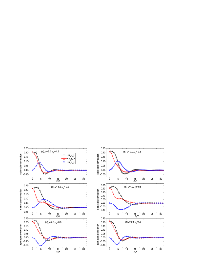
Figure 9: The results of spin-spin correlation with respect to the displacement $k_{T}R$ for the cases that $\epsilon_{d}<\mu$. (a) $\mu=-3.0$, $\epsilon_{d}=-4.5$, (b) $\mu=-2.0$, $\epsilon_{d}=-3.5$, (c) $\mu=-1.0$, $\epsilon_{d}=-2.5$, (d) $\mu=1.0$, $\epsilon_{d}=-0.5$, (e) $\mu=2.0$, $\epsilon_{d}=0.5$, (f) $\mu=3.0$, $\epsilon_{d}=1.5$.

In QMC simulations, the two-impurity spin-spin correlation functions defined in Eq. (27)-(29) are proper quantities to describe the interaction between magnetic impurities. For the weak coupling case where Eq. (21) can be used, one can check that the spin-spin correlation functions can be written as

$$\langle{S_{1}^{y}S_{2}^{y}}\rangle=\frac{e^{-\beta\mathcal{J}_{\parallel}}-e^{\beta\mathcal{J}_{\parallel}}\cosh(2\beta\mathcal{J}_{\perp})}{e^{-\beta\mathcal{J}_{\parallel}}+e^{\beta\mathcal{J}_{\parallel}}\cosh(2\beta\mathcal{J}_{\perp})}m_{d}^{2},$$ (31)

$$\langle{S_{1}^{x}S_{2}^{x}}\rangle=-\frac{\mathcal{K}-\mathcal{Q}}{\mathcal{J}_{\perp}}\frac{e^{\beta\mathcal{J}_{\parallel}}\sinh(2\beta\mathcal{J}_{\perp})}{e^{-\beta\mathcal{J}_{\parallel}}+e^{\beta\mathcal{J}_{\parallel}}\cosh(2\beta\mathcal{J}_{\perp})}m_{d}^{2},$$ (32)

$$\langle{S_{1}^{x}S_{2}^{z}}\rangle=-\frac{\mathcal{R}}{\mathcal{J}_{\perp}}\frac{e^{\beta\mathcal{J}_{\parallel}}\sinh(2\beta\mathcal{J}_{\perp})}{e^{-\beta\mathcal{J}_{\parallel}}+e^{\beta\mathcal{J}_{\parallel}}\cosh(2\beta\mathcal{J}_{\perp})}m_{d}^{2},$$ (33)

where $\mathcal{J}_{\parallel}=\mathcal{K}+\mathcal{Q}$, $\mathcal{J}_{\perp}=\sqrt{(\mathcal{K}-\mathcal{Q})^{2}+\mathcal{R}^{2}}$. In the low temperature region where $\beta\mathcal{K},\beta\mathcal{Q}$ and $\beta\mathcal{R}\ll 1$, the spin-spin correlation functions are proportional to the spin-spin interactions, $\langle{S_{1}^{y}S_{2}^{y}}\rangle\sim-\beta(\mathcal{K}+\mathcal{Q})m_{d}^{2}$, $\langle{S_{1}^{x}S_{2}^{x}}\rangle\sim-\beta(\mathcal{K}-\mathcal{Q})m_{d}^{2}$, $\langle{S_{1}^{x}S_{2}^{z}}\rangle\sim\beta\mathcal{R}m_{d}^{2}$.

Before a more detailed discussion of general spin-spin correlations, we consider the special case $k_{T}R=0$ firstly. Mean-field analysis demonstrate that the anisotropic and the DM-like spin-spin interactions vanishes in this special case. In QMC simulation, we find similar results, the longitudinal and transverse components of the spin-spin correlation defined in Eq. (27) and Eq. (28) have the same values, and the DM-like component vanishes. Fig. (8) shows the numerical results of isotropic spin-spin correlation function. Two issues need to be addressed about Fig. (8). Firstly, when the chemical potential is tuned into the gap (i.e. $-0.5<\mu<0.5$), the correlation between magnetic impurities is suppressed. This is because the correlation is mediated by itinerant electrons. Secondly, the spin-spin correlation can either be FM or AFM, while the mean-field analysis prefers FM correlation for any given parameters (as shown in Fig. (4) and Fig. (5), $\mathcal{K}(0,\mu)<0$).

Now we present the spin-spin correlation with respect to the displacement $k_{T}R$ for some typical values of $\epsilon_{d}$ and $\mu$ (Fig. (9)). In all the cases we test, we fix $\epsilon_{d}-\mu=-1.5$ which most prefer local moment formation when the on-site Coulomb repulsion $U=3.0$. In Fig. (9a)-(9c), we present the results of spin-spin correlation for the cases that the chemical potential is tuned into the valence band. Firstly, similar to the mean-field results, the DM-like correlation $\langle{S_{1}^{x}S_{2}^{z}}\rangle$ and the difference between the longitudinal and transverse correlations tend to zero smoothly in short separation limit. Secondly, the difference between the longitudinal and transverse correlations becomes more apparent as the chemical potential approaches zero. Shown in Fig. (9d)-(9f) are the results of spin-spin correlation when $\mu$ is switched into the conduction band. The FM behavior of the longitudinal and transverse correlations in the short displacement range remain unchanged. However, we can see that the oscillation of $\langle{S_{1}^{x}S_{2}^{z}}\rangle$ are opposite, which is qualitatively consistent with the mean-field results $\mathcal{K}(R,\mu)=\mathcal{K}(R,-\mu)$, $\mathcal{Q}(R,\mu)=\mathcal{Q}(R,-\mu)$ and $\mathcal{R}(R,\mu)=-\mathcal{R}(R,-\mu)$.

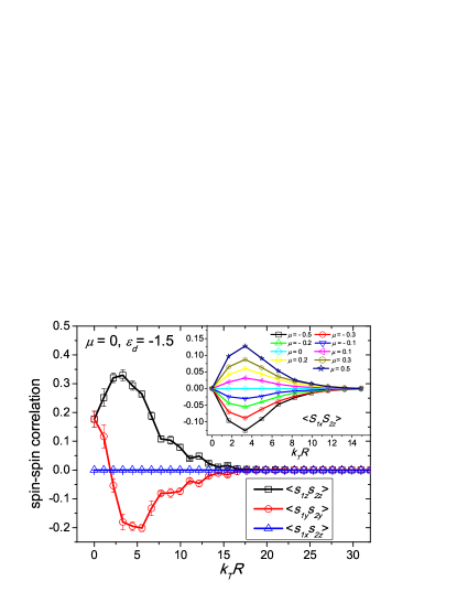
Figure 10: The results of spin-spin correlation with respect to the displacement $k_{T}R$ for $\mu=0$ and $\epsilon_{d}=-1.5$. The inset shows the results of DM-like spin-spin correlation for various values of $\mu$ while $\epsilon_{d}-\mu=-1.5=-U/2$.

In Fig. (10) we show the results of spin-spin correlation when the chemical potential is tuned into the gap of the TIs ($\mu=0$) for $\epsilon_{d}=-1.5$. The first important feature in this figure is that the transverse DM-like correlation is vanished. Theoretically, one can demonstrate that $\langle{S_{1}^{x}S_{2}^{z}}\rangle$ is exactly zero according to the particle-hole symmetry ($\Psi\rightarrow\tau_{y}\sigma_{y}\Psi^{\dagger}$, $d\rightarrow\sigma_{y}{d}^{\dagger}$) and inversion symmetry ($\Psi\rightarrow\tau_{z}\Psi$, $d_{1}\leftrightarrow{d}_{2}$). Actually, under the combined symmetric transformation, one can find that $\langle{S_{1}^{x}S_{2}^{z}}\rangle=\langle{S_{2}^{x}S_{1}^{z}}\rangle$, however, $\langle{S_{1}^{x}S_{2}^{z}}\rangle=-\langle{S_{1}^{z}S_{2}^{x}}\rangle$ according to rotation symmetry, so $\langle{S_{1}^{x}S_{2}^{z}}\rangle=0$. According to our QMC calculations, the values of the DM-like correlation is exactly zero when $\mu=0$ and $\epsilon_{d}=-1.5=-U/2$, which means that our QMC simulations preserve the symmetries exactly. We also find that as the chemical potential approaches zero, the amplitude of the DM-like correlation function decreases for both positive and negative values of $\mu$, as shown in the inset of Fig. (10). The second important feature in Fig. (10) is that the distinction between $\langle{S_{1}^{z}S_{2}^{z}}\rangle$ and $\langle{S_{1}^{y}S_{2}^{y}}\rangle$ is significant when $\mu=0$. One can find that such a distinction is more remarkable than that in the mean-field results (see Fig. (4)).

IV Discussion and conclusion

In this work, we apply mean-field theory and HFQMC method to study the spin-spin interaction in the bulk of TIs. We find that the spin-spin interaction has three different components: the longitudinal, the transverse and the transverse DM-like interaction induced by the spin-orbit coupling. From the mean-field calculation, we find that for a heavy doped system, all three kinds of spin-spin interaction oscillate with the same period $2\pi/\sqrt{|\mu|/mB}$, and decay with $\sim 1/R^{3}$ in the limit $R\rightarrow\infty$. Both the quantum Monte Carlo simulations and mean-field calculations demonstrate that the longitudinal interaction oscillates like the transverse one, and both of them are always ferromagnetic for $\epsilon_{d}<\mu$ in the short range limit, ${k_{T}}R\rightarrow 0$. When the Fermi energy is located in the bulk gap of TIs, the spin-spin interaction decays exponentially due to the Bloembergen-Rowland interaction. The mean-field calculation and the HFQMC simulation demonstrate that (For sufficiently large distance, i.e. $k_{T}R>5$) the longitudinal interaction is antiferromagnetic and transverse ones are ferromagnetic.

For the real material Fe_xBi₂Te₃, if we ignore the influence of anisotropic crystal structure and choose the following parametersLiu et al. (2010): lattice spacing $a=4.38$Å, $v_{F}=2.87$eVÅ and $m=0.3$eV, then $v_{F}{k_{T}}/m\thickapprox 5.53$ and ${k_{T}}a\thickapprox 2.53$. $k_{T}{R}\sim 10$ corresponds to $R{\sim}4a$ and concentration of impurity $x{\sim}0.016$ which defines a typical length scale. When $k_{T}{R}<10$, the difference between longitudinal correlation and transverse correlation and the importance of DM-like correlation become significant (see Fig. (9) and Fig. (5)). However, more detailed analysis, such as the anisotropic lattice structure, the position of magnetic impurities, are required to explain the topological phase transition between ferromagnetic-cluster glassy behavior for $x\sim 0.025$ and valence-bond glassy behavior for $x\sim 0.03$ to $0.1$.

V Acknowledgement

This work is supported by NSAF (Grant No. U1230202), China Postdoctoral Science Foundation (Grant No. 2013M540845), and CAEP.

References

- Fu et al. (2007) L. Fu, C. L. Kane, and E. J. Mele, Phys. Rev. Lett. 98, 106803 (2007).
- Xia et al. (2009) Y. Xia, D. Qian, D. Hsieh, L. Wray, A. Pal, H. Lin, A. Bansil, D. Grauer, Y. S. Hor, R. J. Cava, and M. Z. Hasan, Nat. Phys. 5, 398 (2009).
- Zhang et al. (2009) H. Zhang, C.-X. Liu, X.-L. Qi, X. Dai, Z. Fang, and S.-C. Zhang, Nat. Phys. 5, 438 (2009).
- Moore (2010) J. E. Moore, Nature 464, 194 (2010).
- Hasan and Kane (2010) M. Z. Hasan and C. L. Kane, Rev. Mod. Phys. 82, 3045 (2010).
- Qi and Zhang (2011) X.-L. Qi and S.-C. Zhang, Rev. Mod. Phys. 83, 1057 (2011).
- Qi et al. (2008) X.-L. Qi, T. L. Hughes, and S.-C. Zhang, Phys. Rev. B 78, 195424 (2008).
- Nomura and Nagaosa (2011) K. Nomura and N. Nagaosa, Phys. Rev. Lett. 106, 166802 (2011).
- Qi et al. (2009) X.-L. Qi, R. Li, J. Zang, and S.-C. Zhang, Science 323, 1184 (2009).
- Zang and Nagaosa (2010) J. Zang and N. Nagaosa, Phys. Rev. B 81, 245125 (2010).
- Tse and MacDonald (2010) W.-K. Tse and A. H. MacDonald, Phys. Rev. Lett. 105, 057401 (2010).
- Tse and MacDonald (2011) W.-K. Tse and A. H. MacDonald, Phys. Rev. B 84, 205327 (2011).
- Maciejko et al. (2010) J. Maciejko, X.-L. Qi, H. D. Drew, and S.-C. Zhang, Phys. Rev. Lett. 105, 166803 (2010).
- Lan et al. (2011) Y. Lan, S. Wan, and S.-C. Zhang, Phys. Rev. B 83, 205109 (2011).
- Grushin and Cortijo (2011) A. G. Grushin and A. Cortijo, Phys. Rev. Lett. 106, 020403 (2011).
- Grushin et al. (2011) A. G. Grushin, P. Rodriguez-Lopez, and A. Cortijo, Phys. Rev. B 84, 045119 (2011).
- Chen and Wan (2011) L. Chen and S. Wan, Phys. Rev. B 84, 075149 (2011).
- Chen et al. (2010) Y. L. Chen, J.-H. Chu, J. G. Analytis, Z. K. Liu, K. Igarashi, H.-H. Kuo, X. L. Qi, S. K. Mo, R. G. Moore, D. H. Lu, M. Hashimoto, T. Sasagawa, S. C. Zhang, I. R. Fisher, Z. Hussain, and Z. X. Shen, Science 329, 659 (2010).
- Wray et al. (2011) L. A. Wray, S.-Y. Xu, Y. Xia, D. Hsieh, A. V. Fedorov, Y. S. Hor, R. J. Cava, A. Bansil, H. Lin, and M. Z. Hasan, Nat. Phys. 7, 32 (2011).
- Okada et al. (2011) Y. Okada, C. Dhital, W. Zhou, E. D. Huemiller, H. Lin, S. Basak, A. Bansil, Y.-B. Huang, H. Ding, Z. Wang, S. D. Wilson, and V. Madhavan, Phys. Rev. Lett. 106, 206805 (2011).
- Valla et al. (2012) T. Valla, Z.-H. Pan, D. Gardner, Y. S. Lee, and S. Chu, Phys. Rev. Lett. 108, 117601 (2012).
- Hor et al. (2010) Y. S. Hor, P. Roushan, H. Beidenkopf, J. Seo, D. Qu, J. G. Checkelsky, L. A. Wray, D. Hsieh, Y. Xia, S.-Y. Xu, D. Qian, M. Z. Hasan, N. P. Ong, A. Yazdani, and R. J. Cava, Phys. Rev. B 81, 195203 (2010).
- Scholz et al. (2012) M. R. Scholz, J. Sánchez-Barriga, D. Marchenko, A. Varykhalov, A. Volykhov, L. V. Yashina, and O. Rader, Phys. Rev. Lett. 108, 256810 (2012).
- Kasuya (1956) T. Kasuya, Progress of Theoretical Physics 16, 45 (1956).
- Ruderman and Kittel (1954) M. A. Ruderman and C. Kittel, Phys. Rev. 96, 99 (1954).
- Yosida (1957) K. Yosida, Phys. Rev. 106, 893 (1957).
- Liu et al. (2009) Q. Liu, C.-X. Liu, C. Xu, X.-L. Qi, and S.-C. Zhang, Phys. Rev. Lett. 102, 156603 (2009).
- Zhu et al. (2011) J.-J. Zhu, D.-X. Yao, S.-C. Zhang, and K. Chang, Phys. Rev. Lett. 106, 097201 (2011).
- Abanin and Pesin (2011) D. A. Abanin and D. A. Pesin, Phys. Rev. Lett. 106, 136802 (2011).
- Biswas and Balatsky (2010) R. R. Biswas and A. V. Balatsky, Phys. Rev. B 81, 233405 (2010).
- Lü et al. (2013) H.-F. Lü, H.-Z. Lu, S.-Q. Shen, and T.-K. Ng, Phys. Rev. B 87, 195122 (2013).
- Rosenberg and Franz (2012) G. Rosenberg and M. Franz, Phys. Rev. B 85, 195119 (2012).
- Schmidt et al. (2011) T. M. Schmidt, R. H. Miwa, and A. Fazzio, Phys. Rev. B 84, 245418 (2011).
- Henk et al. (2012) J. Henk, A. Ernst, S. V. Eremeev, E. V. Chulkov, I. V. Maznichenko, and I. Mertig, Phys. Rev. Lett. 108, 206801 (2012).
- Zhang et al. (2012) J.-M. Zhang, W. Zhu, Y. Zhang, D. Xiao, and Y. Yao, Phys. Rev. Lett. 109, 266405 (2012).
- Kim et al. (2013) H.-J. Kim, K.-S. Kim, J.-F. Wang, V. A. Kulbachinskii, K. Ogawa, M. Sasaki, A. Ohnishi, M. Kitaura, Y.-Y. Wu, L. Li, I. Yamamoto, J. Azuma, M. Kamada, and V. Dobrosavljević, Phys. Rev. Lett. 110, 136601 (2013).
- Hirsch and Fye (1986) J. E. Hirsch and R. M. Fye, Phys. Rev. Lett. 56, 2521 (1986).
- Anderson (1961) P. W. Anderson, Phys. Rev. 124, 41 (1961).
- Haldane and Anderson (1976) F. D. M. Haldane and P. W. Anderson, Phys. Rev. B 13, 2553 (1976).
- Uchoa et al. (2008) B. Uchoa, V. N. Kotov, N. M. R. Peres, and A. H. Castro Neto, Phys. Rev. Lett. 101, 026805 (2008).
- Negele and Orland (1998) J. W. Negele and H. Orland, Quantum Many Particle Systems (Westview Press, 1998).
- Fye and Hirsch (1988) R. M. Fye and J. E. Hirsch, Phys. Rev. B 38, 433 (1988).
- Fye et al. (1987) R. M. Fye, J. E. Hirsch, and D. J. Scalapino, Phys. Rev. B 35, 4901 (1987).
- Hirsch and Lin (1987) J. E. Hirsch and H. Q. Lin, Phys. Rev. B 35, 4943 (1987).
- Bulut et al. (2007) N. Bulut, K. Tanikawa, S. Takahashi, and S. Maekawa, Phys. Rev. B 76, 045220 (2007).
- Hu et al. (2011) F. M. Hu, T. Ma, H.-Q. Lin, and J. E. Gubernatis, Phys. Rev. B 84, 075414 (2011).
- Lu et al. (2010) H.-Z. Lu, W.-Y. Shan, W. Yao, Q. Niu, and S.-Q. Shen, Phys. Rev. B 81, 115407 (2010).
- Shan et al. (2010) W.-Y. Shan, H.-Z. Lu, and S.-Q. Shen, New Journal of Physics 12, 043048 (2010).
- Shen et al. (2011) S.-Q. Shen, W.-Y. Shan, and H.-Z. Lu, SPIN 01, 33 (2011).
- Hewson (1997) A. C. Hewson, The Kondo Problem to Heavy Fermions (Cambridge University Press, 1997).
- Hsieh et al. (2009) D. Hsieh, Y. Xia, D. Qian, L. Wray, J. H. Dil, F. Meier, J. Osterwalder, L. Patthey, J. G. Checkelsky, N. P. Ong, A. V. Fedorov, H. Lin, A. Bansil, D. Grauer, Y. S. Hor, R. J. Cava, and M. Z. Hasan, Nature 460, 1101 (2009).
- Tsvelik (2007) A. M. Tsvelik, Quantum Field Theory in Condensed Matter Physics (Cambridge University Press, 2007).
- Liu et al. (2010) C.-X. Liu, X.-L. Qi, H. Zhang, X. Dai, Z. Fang, and S.-C. Zhang, Phys. Rev. B 82, 045122 (2010).