Coupling layers regularizes wave propagation in laminar stochastic neural fields

Zachary P. Kilpatrick zpkilpat@math.uh.edu Department of Mathematics, University of Houston, Houston, TX 77204
Abstract

We study the effects of coupling between layers of stochastic neural field models with laminar structure. In particular, we focus on how the propagation of waves of neural activity in each layer is affected by the coupling. Synaptic connectivities within and between each layer are determined by integral kernels of an integrodifferential equation describing the temporal evolution of neural activity. Excitatory neural fields, with purely positive connectivities, support traveling fronts in each layer, whose speeds are increased when coupling between layers is considered. Studying the effects of noise, we find coupling also serves to reduce the variance in the position of traveling fronts, as long as the noise sources to each layer are not completely correlated. Neural fields with asymmetric connectivity support traveling pulses whose speeds are decreased by interlaminar coupling. Again, coupling reducers the variance in traveling pulse position, when noise is considered that is not totally correlated between layers. To derive our stochastic results, we employ a small-noise expansion, also assuming inter-laminar connectivity scales similarly. Our asymptotic results agree reasonably with accompanying numerical simulations.

I Introduction

There is a growing experimental literature describing the detailed functional architecture of large scale neuronal networks Sporns et al. (2004). Much recent development is due to innovative techniques in neural recording such as voltage sensitive dye Ferezou et al. (2007), high capacity multielectrodes Nicolelis et al. (2003), and optogenetics Zhang et al. (2010). Modern electrophysiology reaches well beyond classic neuroanatomical approaches, and details about the complex organization of brain networks in the brain are coming to light Bullmore and Sporns (2009). One particular organizational motif shown to be important for sensory processing is a layered, or laminar, organization of cortical tissue, identified decades ago in visual cortex Hubel and Wiesel (1977). An important component of this type of architecture is that synaptic connections between layers have some topographic organization, reflecting recurrent architecture of each local layer Felleman and Van Essen (1991). Laminar architecture has now been identified as an important part of motor Weiler et al. (2008), somatosensory Shepherd and Svoboda (2005), and spatial memory McNaughton et al. (2006) processing. This contributes to previous findings, that connectivity across multiple areas of the brain is important for neural computations like working memory Curtis (2006), visual processing Bullier (2001), and attention Luck et al. (1997).

The structure of network organization strongly influences the wide variety of spatiotemporal activity patterns observed throughout the brain Wang (2010). Strong local recurrent excitation can reenforce stimulus tuning of local assemblies of neurons Song et al. (2005), elevating the local response to external inputs Ferster and Miller (2000), even allowing neural activity to persist seconds after after a stimulus is removed Goldman-Rakic (1995). In addition, inhibition is known to be dense in many areas of cortex Fino and Yuste (2011), resulting in sharper spatiotemporal responses to sensory stimuli Wehr and Zador (2003). In addition to relating synaptic polarity to local cortical dynamics, the intricate spatial architecture of many networks in cortex governs those regions’ resulting spatiotemporal activity Gilbert et al. (1996); Witter and Moser (2006); Vincent et al. (2007). For instance, recordings from developing cerebellum reveal that spatial asymmetries in excitatory connectivity can lead to traveling waves of activity Watt et al. (2009). Propagating waves of activity have been observed in many sensory cortices Ermentrout and Kleinfeld (2001); Petersen et al. (2003); Huang et al. (2004); Rubino et al. (2006), presumed to amplify or mark the timing of incoming signals. Typically, computational models presume they arise from a combination of recurrent excitation and negative feedback like spike rate adaptation Pinto and Ermentrout (2001) or short term depression Kilpatrick and Bressloff (2010a).

Therefore, there are a number of established principles concerning how different architectural motifs shape the brain’s spatiotemporal activity patterns. We will extend this work by exploring how laminar architecture affects the propagation of activity in stochastic neuronal networks. Recently, we showed that laminar architecture in models of spatial working memory can help stabilize persistent localized activity in the presence of fluctuations Kilpatrick (2013). Persistent activity, in the form of localized bumps, executes a random walk when stochastic fluctuations are considered, but several coupled bumps can cancel much of this noise due to the attractive force between their positions. In this work, similar principles will be demonstrated in stochastic neuronal networks that support traveling waves. Our interest will be in traveling waves that arise from two different mechanisms.

First, we will consider traveling waves in purely excitatory neuronal networks, often used as models for disinhibited cortical slices Richardson et al. (2005). Here, the speed of traveling waves is determined by the activity threshold of the network. Second, we will consider traveling waves in asymmetric neuronal networks, previously used as models of direction selectivity Xie and Giese (2002). The skew of the asymmetry in spatial connectivity determines the speed of traveling waves in these model. Typically, neural field models only consider a single layer of cortical tissue, sometimes separated into distinct excitatory and inhibitory populations Bressloff (2012). However, some recent modeling efforts accounted for the multi-laminar structure of cortex, applying them to study interacting bumps Folias and Ermentrout (2011) and binocular rivalry Kilpatrick and Bressloff (2010b); Bressloff and Webber (2012a). Here, we will combine this approach with a consideration of stochasticity on wave propagation.

There are a number of recent mathematical studies considering how stochasticity affects the formation of spatiotemporal patterns in neuronal networks. Turing patterns Hutt et al. (2007), traveling fronts Bressloff and Webber (2012b), and stationary bumps Kilpatrick and Ermentrout (2013) can all be analyzed in stochastic neural fields with the aid of small-noise expansions originally developed to analyze wave propagation in stochastic partial differential equations Armero et al. (1998). Such an approach typically results in a diffusion equation for the position of the spatiotemporal activity, but upon considering a neural field with multiple layers, the effective equations are multivariate Ornstein-Uhlenbeck processes instead Kilpatrick (2013). Thus, the small-noise expansion allows one to examine the effects of connectivity between layers, in addition to noise. Since recordings of cortical activity are becoming substantially more detailed Nicolelis et al. (2003); Zhang et al. (2010), the time is ripe for extending theories of spatiotemporal activity patterns in cortex.

The paper will proceed as follows. In section II, we introduce the models we explore, showing how noise and a multi-laminar structure can be introduced into neural field models Hutt et al. (2007). One important point is that the correlation structure of spatiotemporal noise can be tuned in the model, and changing this has non-trivial effects on the resulting dynamics. We proceed, in section III, to show how a combination of interlaminar connectivity along with noise affects the propagation of traveling fronts in an excitatory neural field model. As in Kilpatrick (2013), we are able to derive an effective equation for the position of the front, which takes the form of a multivariate OU process. Finally, we derive similar results for traveling pulse propagation in asymmetric neural fields in section IV.

II Laminar neural field model

We will consider two different models for wave propagation in neural fields. They both take the form of a system of coupled stochastic neural field equations

du1(x,t)=dsubscript𝑢1𝑥𝑡absent\displaystyle{\rm d}u_{1}(x,t)= [u1+k=12w1kf(uk)]dt+ε1/2dW1(x,t),delimited-[]subscript𝑢1superscriptsubscript𝑘12subscript𝑤1𝑘𝑓subscript𝑢𝑘d𝑡superscript𝜀12dsubscript𝑊1𝑥𝑡\displaystyle\left[-u_{1}+\sum_{k=1}^{2}w_{1k}*f(u_{k})\right]{\rm d}t+\varepsilon^{1/2}{\rm d}W_{1}(x,t), (1a)
du2(x,t)=dsubscript𝑢2𝑥𝑡absent\displaystyle{\rm d}u_{2}(x,t)= [u2+k=12w2kf(uk)]dt+ε1/2dW2(x,t),delimited-[]subscript𝑢2superscriptsubscript𝑘12subscript𝑤2𝑘𝑓subscript𝑢𝑘d𝑡superscript𝜀12dsubscript𝑊2𝑥𝑡\displaystyle\left[-u_{2}+\sum_{k=1}^{2}w_{2k}*f(u_{k})\right]{\rm d}t+\varepsilon^{1/2}{\rm d}W_{2}(x,t), (1b)

where uj(x,t)subscript𝑢𝑗𝑥𝑡u_{j}(x,t) is the neural activity of population j𝑗j at xΩ𝑥Ωx\in\Omega at time t𝑡t, and the effects of synaptic architecture are describe by the convolution

wjkf(uk)=Ωwjk(xy)f(uk(y))dy,subscript𝑤𝑗𝑘𝑓subscript𝑢𝑘subscriptΩsubscript𝑤𝑗𝑘𝑥𝑦𝑓subscript𝑢𝑘𝑦differential-d𝑦\displaystyle w_{jk}*f(u_{k})=\int_{\Omega}w_{jk}(x-y)f(u_{k}(y)){\rm d}y,

for j,k=1,2formulae-sequence𝑗𝑘12j,k=1,2, so the case j=k𝑗𝑘j=k describes recurrent synaptic connections within a layer and jk𝑗𝑘j\neq k describes synaptic connections between layers (interlaminar). The function wjk(xy)subscript𝑤𝑗𝑘𝑥𝑦w_{jk}(x-y) describes the strength (amplitude of wjksubscript𝑤𝑗𝑘w_{jk}) and net polarity (sign of wjksubscript𝑤𝑗𝑘w_{jk}) of synaptic interactions from neurons with stimulus preference y𝑦y to those with preference x𝑥x. For our analysis of traveling fronts, we consider positive, even weight functions for wjksubscript𝑤𝑗𝑘w_{jk}. In particular, we will take the exponential function

wjk(xy)=w¯jk2e|xy|,subscript𝑤𝑗𝑘𝑥𝑦subscript¯𝑤𝑗𝑘2superscripte𝑥𝑦\displaystyle w_{jk}(x-y)=\frac{\bar{w}_{jk}}{2}{\rm e}^{-|x-y|}, (2)

so that w¯jksubscript¯𝑤𝑗𝑘\bar{w}_{jk} parametrizes the total strength of connections from population k𝑘k to j𝑗j. Studying excitatory neural fields in section III, we extend the spatial domain to Ω=(,)Ω\Omega=(-\infty,\infty). In our analysis of coupled traveling pulses in section IV, we presume the modulation of the recurrent synaptic strength is given by the shifted cosine

wjj(xy)=cos(xyϕj),j=1,2,formulae-sequencesubscript𝑤𝑗𝑗𝑥𝑦𝑥𝑦subscriptitalic-ϕ𝑗𝑗12\displaystyle w_{jj}(x-y)=\cos(x-y-\phi_{j}),\ \ \ \ j=1,2, (3)

where ϕjsubscriptitalic-ϕ𝑗\phi_{j} is the amplitude of the shift in the j𝑗jth layer, and the spatial domain is taken to be a periodic ring Ω=[π,π]Ω𝜋𝜋\Omega=[-\pi,\pi]. On the other hand, interlaminar connectivity will generally be given by the pure cosine function

wjk(xy)=w¯jkcos(xy),kj.formulae-sequencesubscript𝑤𝑗𝑘𝑥𝑦subscript¯𝑤𝑗𝑘𝑥𝑦𝑘𝑗\displaystyle w_{jk}(x-y)=\bar{w}_{jk}\cos(x-y),\ \ \ k\neq j. (4)

Presuming that (1) along with (3) is meant to model directionally selective network, maintaining isotropic coupling between layers reflects a common spatial mapping in the positions within each layer.

Output firing rates are given by taking the gain function f(u)𝑓𝑢f(u) of the synaptic input, which are typically considered to be sigmoidal Wilson and Cowan (1973)

f(u)=11+eη(uθ),𝑓𝑢11superscripte𝜂𝑢𝜃\displaystyle f(u)=\frac{1}{1+{\rm e}^{-\eta(u-\theta)}}, (5)

and we will often take the high gain limit (η𝜂\eta\to\infty), which allows the explicit computation of quantities of interest Amari (1977)

f(u)=H(uθ)={1:u>θ,0:u<θ.𝑓𝑢𝐻𝑢𝜃cases1:absent𝑢𝜃0:absent𝑢𝜃\displaystyle f(u)=H(u-\theta)=\left\{\begin{array}[]{cl}1&:u>\theta,\\ 0&:u<\theta.\end{array}\right. (8)

Spatiotemporal noises are described by small amplitude (ε1much-less-than𝜀1\varepsilon\ll 1) stochastic processes ε1/2Wj(x,t)superscript𝜀12subscript𝑊𝑗𝑥𝑡\varepsilon^{1/2}W_{j}(x,t) that are white in time dWj(x,t)=0delimited-⟨⟩dsubscript𝑊𝑗𝑥𝑡0\langle{\rm d}W_{j}(x,t)\rangle=0 and correlated in space

dWj(x,t)dWj(y,s)delimited-⟨⟩dsubscript𝑊𝑗𝑥𝑡dsubscript𝑊𝑗𝑦𝑠\displaystyle\langle{\rm d}W_{j}(x,t){\rm d}W_{j}(y,s)\rangle =Cj(xy)δ(ts)dtds,j=1,2,formulae-sequenceabsentsubscript𝐶𝑗𝑥𝑦𝛿𝑡𝑠d𝑡d𝑠𝑗12\displaystyle=C_{j}(x-y)\delta(t-s){\rm d}t{\rm d}s,\ \ \ j=1,2,
dWj(x,t)dWk(y,s)delimited-⟨⟩dsubscript𝑊𝑗𝑥𝑡dsubscript𝑊𝑘𝑦𝑠\displaystyle\langle{\rm d}W_{j}(x,t){\rm d}W_{k}(y,s)\rangle =Cc(xy)δ(ts)dtds,jk,formulae-sequenceabsentsubscript𝐶𝑐𝑥𝑦𝛿𝑡𝑠d𝑡d𝑠𝑗𝑘\displaystyle=C_{c}(x-y)\delta(t-s){\rm d}t{\rm d}s,\ \ \ j\neq k,

describing local and shared noise in either layer, j=1,2𝑗12j=1,2. To demonstrate our theory, we can examine the effects of the simple case of spatially homogeneous noise Cj(xy)=χjsubscript𝐶𝑗𝑥𝑦subscript𝜒𝑗C_{j}(x-y)=\chi_{j} and Cc(xy)=χcsubscript𝐶𝑐𝑥𝑦subscript𝜒𝑐C_{c}(x-y)=\chi_{c}. In addition, we can assume a local spatial correlations have a cosine profile Cj(x)=χjcos(x/σ)subscript𝐶𝑗𝑥subscript𝜒𝑗𝑥𝜎C_{j}(x)=\chi_{j}\cos(x/\sigma), along with correlated noise component with a cosine profile so Cc(x)=χccos(x/σ)subscript𝐶𝑐𝑥subscript𝜒𝑐𝑥𝜎C_{c}(x)=\chi_{c}\cos(x/\sigma). Therefore, in the limit χc0subscript𝜒𝑐0\chi_{c}\to 0, there are no interlaminar noise correlations, and in the limit χcmax(χ1,χ2)subscript𝜒𝑐subscript𝜒1subscript𝜒2\chi_{c}\to\max(\chi_{1},\chi_{2}), noise in each layer is maximally correlated.

III Dual layer excitatory network

III.1 Coupled front propagation

To begin we examine a network of two coupled excitatory layers, which individually produce propagating fronts. In the presence of sufficient coupling between layers, we will show their front speeds coincide. This analysis should be contrasted with that in Bressloff and Webber (2012a), which explored fronts coupled with depressing inhibition as a means of modeling binocular rivalry waves. While our stochastic analysis will only consider the effects of weak coupling, our analysis of the effect of coupling on speed will study the effect of arbitrarily strong coupling. Before analyzing front solutions, it is useful to look at spatially homogeneous solutions of the system (1) in the presence of purely excitatory connections, as they govern the limiting values of traveling fronts. Thus, considering constant solutions (u1(x,t),u2(x,t))=(U1¯,U2¯)subscript𝑢1𝑥𝑡subscript𝑢2𝑥𝑡¯subscript𝑈1¯subscript𝑈2(u_{1}(x,t),u_{2}(x,t))=(\bar{U_{1}},\bar{U_{2}}), upon plugging them into (1), we have

U1¯¯subscript𝑈1\displaystyle\bar{U_{1}} =f(U1¯)w¯11+f(U2¯)w¯12absent𝑓¯subscript𝑈1subscript¯𝑤11𝑓¯subscript𝑈2subscript¯𝑤12\displaystyle=f(\bar{U_{1}})\bar{w}_{11}+f(\bar{U_{2}})\bar{w}_{12}
U2¯¯subscript𝑈2\displaystyle\bar{U_{2}} =f(U2¯)w¯22+f(U1¯)w¯21,absent𝑓¯subscript𝑈2subscript¯𝑤22𝑓¯subscript𝑈1subscript¯𝑤21\displaystyle=f(\bar{U_{2}})\bar{w}_{22}+f(\bar{U_{1}})\bar{w}_{21}, (9)

where w¯jk=wjk(x)dx0subscript¯𝑤𝑗𝑘superscriptsubscriptsubscript𝑤𝑗𝑘𝑥differential-d𝑥0\bar{w}_{jk}=\int_{-\infty}^{\infty}w_{jk}(x){\rm d}x\geq 0 since wjksubscript𝑤𝑗𝑘w_{jk} are generally positive, even functions. In the limit w¯12,w¯210subscript¯𝑤12subscript¯𝑤210\bar{w}_{12},\bar{w}_{21}\to 0 and f𝑓f is a sufficiently steep sigmoid (5) , it can be shown that each equation in (9) will have three roots Ermentrout and McLeod (1993). The largest (U¯1+subscript¯𝑈limit-from1\bar{U}_{1+} and U¯2+subscript¯𝑈limit-from2\bar{U}_{2+}) and smallest (U¯1subscript¯𝑈limit-from1\bar{U}_{1-} and U¯2subscript¯𝑈limit-from2\bar{U}_{2-}) of these constitute the boundary conditions of corresponding traveling wave solutions. Thus, as w¯12,w¯21subscript¯𝑤12subscript¯𝑤21\bar{w}_{12},\bar{w}_{21} are increased from zero, we expect this fact to still hold over a substantial range of parameters.

Thus, we seek to construct coupled traveling front solutions to (1) by converting the system to the traveling coordinate frame ξ=xct𝜉𝑥𝑐𝑡\xi=x-ct, where the wave speed c𝑐c is yet to be determined. Violations of this assumption will be bifurcations from coupled traveling front solutions. Thus, traveling fronts take the form (u1(x,t),u2(x,t))=(U1(ξ),U2(ξ))subscript𝑢1𝑥𝑡subscript𝑢2𝑥𝑡subscript𝑈1𝜉subscript𝑈2𝜉(u_{1}(x,t),u_{2}(x,t))=(U_{1}(\xi),U_{2}(\xi)). The translation invariance of the system allows us to set the leading edge of the first front to be at ξ=0𝜉0\xi=0 to ease calculations, so they satisfy

cU1(ξ)𝑐superscriptsubscript𝑈1𝜉\displaystyle-cU_{1}^{\prime}(\xi) =U1(ξ)+w11f(U1)+w12f(U2),absentsubscript𝑈1𝜉subscript𝑤11𝑓subscript𝑈1subscript𝑤12𝑓subscript𝑈2\displaystyle=-U_{1}(\xi)+w_{11}*f(U_{1})+w_{12}*f(U_{2}), (10)
cU2(ξ)𝑐superscriptsubscript𝑈2𝜉\displaystyle-cU_{2}^{\prime}(\xi) =U2(ξ)+w22f(U2)+w21f(U1),absentsubscript𝑈2𝜉subscript𝑤22𝑓subscript𝑈2subscript𝑤21𝑓subscript𝑈1\displaystyle=-U_{2}(\xi)+w_{22}*f(U_{2})+w_{21}*f(U_{1}), (11)

where the convolution * is over Ω=(,)Ω\Omega=(-\infty,\infty) with the boundedness conditions limξ±U1(ξ)=U¯1±subscript𝜉plus-or-minussubscript𝑈1𝜉subscript¯𝑈limit-from1plus-or-minus\lim_{\xi\to\pm\infty}U_{1}(\xi)=\bar{U}_{1\pm} and limξ±U2(ξ)=U¯2±subscript𝜉plus-or-minussubscript𝑈2𝜉subscript¯𝑈limit-from2plus-or-minus\lim_{\xi\to\pm\infty}U_{2}(\xi)=\bar{U}_{2\pm}. The set of equations (10) and (11) could be solved using shooting methods for an arbitrary choice of nonlinearity f𝑓f Ermentrout and McLeod (1993); Pinto and Ermentrout (2001) to specify the wavespeed c𝑐c. However, to demonstrate the relationships between parameters will be proceed by assuming the nonlinearity is Heaviside (8). Since we are constructing coupled traveling fronts, there should be a single threshold crossing point for each, yielding the additional conditions U1(0)=U2(a)=θsubscript𝑈10subscript𝑈2𝑎𝜃U_{1}(0)=U_{2}(a)=\theta. We can set the threshold crossing point of U1subscript𝑈1U_{1} due to the underlying translation invariance of (1). Note also the threshold crossing point of U2subscript𝑈2U_{2} need not be the same. Thus, we find equations (10) and (11) become

cU1(ξ)𝑐superscriptsubscript𝑈1𝜉\displaystyle-cU_{1}^{\prime}(\xi) =U1(ξ)+G1(ξ),absentsubscript𝑈1𝜉subscript𝐺1𝜉\displaystyle=-U_{1}(\xi)+G_{1}(\xi), (12)
cU2(ξ)𝑐superscriptsubscript𝑈2𝜉\displaystyle-cU_{2}^{\prime}(\xi) =U2(ξ)+G2(ξ),absentsubscript𝑈2𝜉subscript𝐺2𝜉\displaystyle=-U_{2}(\xi)+G_{2}(\xi), (13)

where

G1(x)subscript𝐺1𝑥\displaystyle G_{1}(x) =xw11(y)dy+xaw12(y)dy,absentsuperscriptsubscript𝑥subscript𝑤11𝑦differential-d𝑦superscriptsubscript𝑥𝑎subscript𝑤12𝑦differential-d𝑦\displaystyle=\int_{x}^{\infty}w_{11}(y){\rm d}y+\int_{x-a}^{\infty}w_{12}(y){\rm d}y,
G2(x)subscript𝐺2𝑥\displaystyle G_{2}(x) =xaw22(y)dy+xw21(y)dy.absentsuperscriptsubscript𝑥𝑎subscript𝑤22𝑦differential-d𝑦superscriptsubscript𝑥subscript𝑤21𝑦differential-d𝑦\displaystyle=\int_{x-a}^{\infty}w_{22}(y){\rm d}y+\int_{x}^{\infty}w_{21}(y){\rm d}y.

Thus, we can integrate the two equations (12) and (13) and apply the threshold conditions U1(0)=θsubscript𝑈10𝜃U_{1}(0)=\theta and U2(a)=θsubscript𝑈2𝑎𝜃U_{2}(a)=\theta to yield

U1(ξ)subscript𝑈1𝜉\displaystyle U_{1}(\xi) =eξ/c(θ1c0ξey/cG1(y)dy),absentsuperscripte𝜉𝑐𝜃1𝑐superscriptsubscript0𝜉superscripte𝑦𝑐subscript𝐺1𝑦differential-d𝑦\displaystyle={\rm e}^{\xi/c}\left(\theta-\frac{1}{c}\int_{0}^{\xi}{\rm e}^{-y/c}G_{1}(y){\rm d}y\right),
U2(ξ)subscript𝑈2𝜉\displaystyle U_{2}(\xi) =eξ/c(θea/c1caξey/cG2(y)dy).absentsuperscripte𝜉𝑐𝜃superscripte𝑎𝑐1𝑐superscriptsubscript𝑎𝜉superscripte𝑦𝑐subscript𝐺2𝑦differential-d𝑦\displaystyle={\rm e}^{\xi/c}\left(\theta{\rm e}^{-a/c}-\frac{1}{c}\int_{a}^{\xi}{\rm e}^{-y/c}G_{2}(y){\rm d}y\right). (14)

Requiring a bounded solution as ξ𝜉\xi\to\infty, assuming c>0𝑐0c>0, we have the conditions

θ𝜃\displaystyle\theta =1c0ey/cG1(y)dy,absent1𝑐superscriptsubscript0superscripte𝑦𝑐subscript𝐺1𝑦differential-d𝑦\displaystyle=\frac{1}{c}\int_{0}^{\infty}{\rm e}^{-y/c}G_{1}(y){\rm d}y,
θ𝜃\displaystyle\theta =ea/ccaey/cG2(y)dy,absentsuperscripte𝑎𝑐𝑐superscriptsubscript𝑎superscripte𝑦𝑐subscript𝐺2𝑦differential-d𝑦\displaystyle=\frac{{\rm e}^{a/c}}{c}\int_{a}^{\infty}{\rm e}^{-y/c}G_{2}(y){\rm d}y, (15)

so plugging (15) into (14) implies

U1(ξ)subscript𝑈1𝜉\displaystyle U_{1}(\xi) =1c0ey/cG1(y+ξ)dy,absent1𝑐superscriptsubscript0superscripte𝑦𝑐subscript𝐺1𝑦𝜉differential-d𝑦\displaystyle=\frac{1}{c}\int_{0}^{\infty}{\rm e}^{-y/c}G_{1}(y+\xi){\rm d}y, (16)
U2(ξ)subscript𝑈2𝜉\displaystyle U_{2}(\xi) =1c0ey/cG2(y+ξ)dy.absent1𝑐superscriptsubscript0superscripte𝑦𝑐subscript𝐺2𝑦𝜉differential-d𝑦\displaystyle=\frac{1}{c}\int_{0}^{\infty}{\rm e}^{-y/c}G_{2}(y+\xi){\rm d}y. (17)

In the case that wjksubscript𝑤𝑗𝑘w_{jk} are all defined as exponential weight distributions (2) with recurrent weighting w¯11=w¯22=1subscript¯𝑤11subscript¯𝑤221\bar{w}_{11}=\bar{w}_{22}=1, the wavespeed c𝑐c and crossing point a𝑎a can be related to the threshold θ𝜃\theta and coupling parameters w¯12subscript¯𝑤12\bar{w}_{12} and w¯21subscript¯𝑤21\bar{w}_{21} by the implicit system

θ𝜃\displaystyle\theta =12(c+1)+w¯12(c,a),absent12𝑐1subscript¯𝑤12𝑐𝑎\displaystyle=\frac{1}{2(c+1)}+\bar{w}_{12}{\mathcal{H}}(c,-a), (18)
θ𝜃\displaystyle\theta =12(c+1)+w¯21(c,+a),absent12𝑐1subscript¯𝑤21𝑐𝑎\displaystyle=\frac{1}{2(c+1)}+\bar{w}_{21}{\mathcal{H}}(c,+a), (19)

where

(c,x)={ex2(c+1):x>0,1+ex2(c1)c2ex/cc21:x<0.𝑐𝑥casessuperscripte𝑥2𝑐1:absent𝑥01superscripte𝑥2𝑐1superscript𝑐2superscripte𝑥𝑐superscript𝑐21:absent𝑥0\displaystyle{\mathcal{H}}(c,x)=\left\{\begin{array}[]{cl}\frac{\displaystyle{\rm e}^{-x}}{\displaystyle 2(c+1)}&:x>0,\\ 1+\frac{\displaystyle{\rm e}^{x}}{\displaystyle 2(c-1)}-\frac{\displaystyle c^{2}{\rm e}^{x/c}}{\displaystyle c^{2}-1}&:x<0.\end{array}\right.

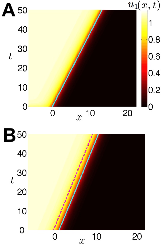
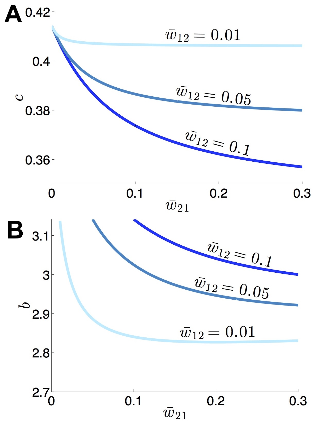
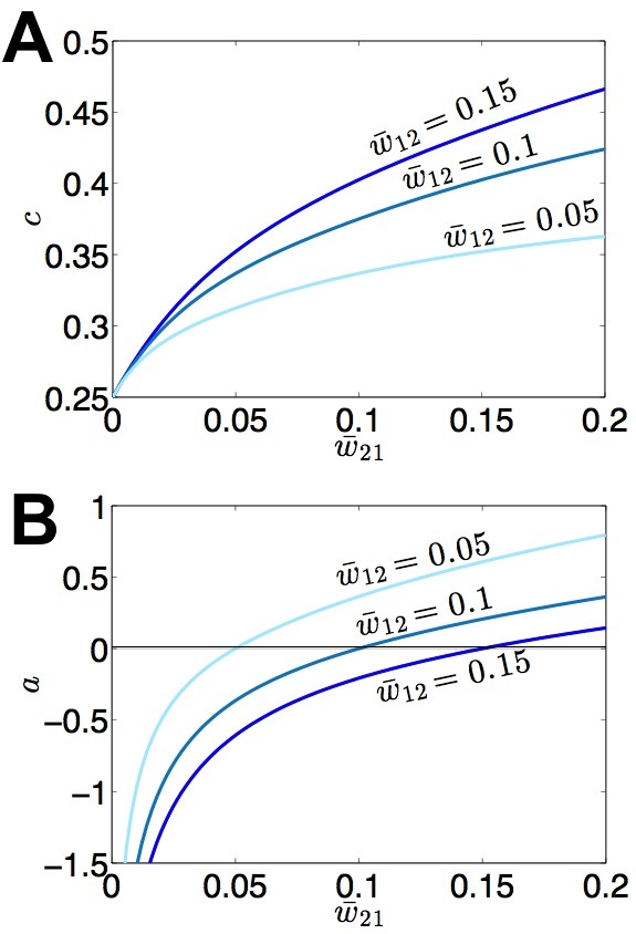
We solve the system (18) and (19) across a range of value of coupling in Fig. 1, showing that the layer receiving more input possesses the leading front. Note, keeping w¯12>0subscript¯𝑤120\bar{w}_{12}>0 fixed, in the limit w¯210subscript¯𝑤210\bar{w}_{21}\to 0, a𝑎a\to-\infty, so when one layer receives much more excitatory input, its front stays far ahead of the other’s. In the case where w¯12=w¯21=w¯csubscript¯𝑤12subscript¯𝑤21subscript¯𝑤𝑐\bar{w}_{12}=\bar{w}_{21}=\bar{w}_{c}, the system simplifies to a single equation, since the front solution U1(ξ)=U2(ξ)subscript𝑈1𝜉subscript𝑈2𝜉U_{1}(\xi)=U_{2}(\xi) exists, due to reflection symmetry of the full system (1) here. Therefore, a=0𝑎0a=0, so we can write

θ=1+w¯c2(c+1)c=1+w¯c2θ1,formulae-sequence𝜃1subscript¯𝑤𝑐2𝑐1𝑐1subscript¯𝑤𝑐2𝜃1\displaystyle\theta=\frac{1+\bar{w}_{c}}{2(c+1)}\ \ \ \ \Rightarrow\ \ \ \ c=\frac{1+\bar{w}_{c}}{2\theta}-1,

so excitatory coupling (w¯c>0subscript¯𝑤𝑐0\bar{w}_{c}>0) between layers increases the speed c𝑐c of both fronts. Finally, in the limit w¯c0subscript¯𝑤𝑐0\bar{w}_{c}\to 0, there are two decoupled fronts, both with speed c=1/(2θ)1𝑐12𝜃1c=1/(2\theta)-1. This is the limit from which we will build our theory of stochastically driven coupled fronts.
Refer to caption
Figure 1: A Speed c𝑐c and B position parameter a𝑎a of coupled traveling fronts (16) and (17) as determined by the implicit system (18) and (19). Notice a=0𝑎0a=0 when w¯21=w¯12subscript¯𝑤21subscript¯𝑤12\bar{w}_{21}=\bar{w}_{12}. Other parameters w¯12=0.1subscript¯𝑤120.1\bar{w}_{12}=0.1 and θ=0.4𝜃0.4\theta=0.4.
Refer to caption
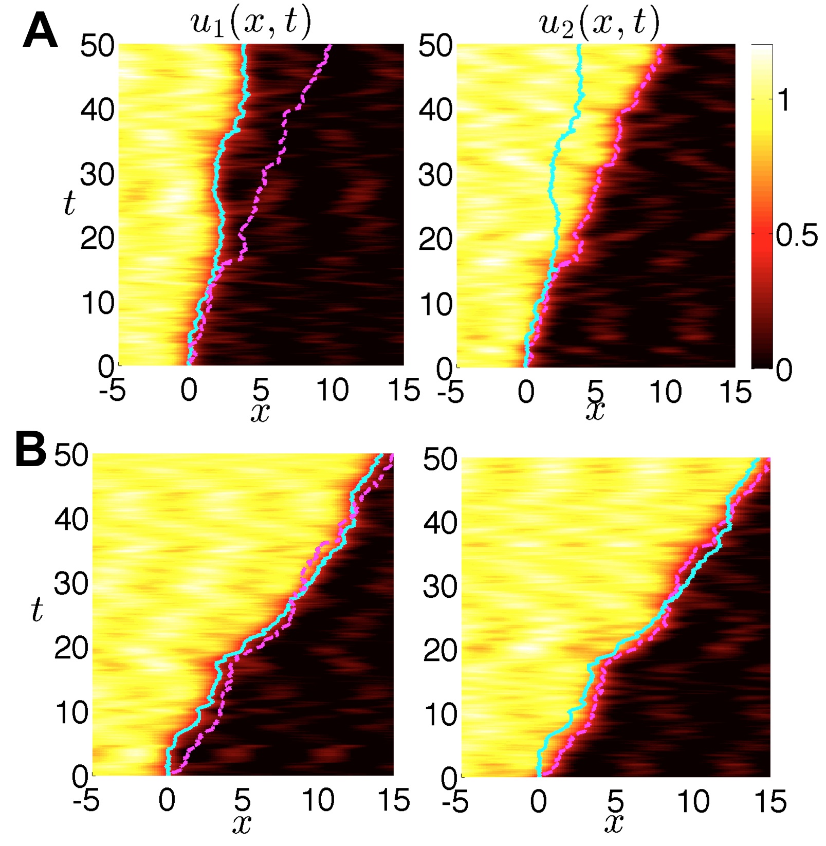
Figure 2: Evolution of coupled fronts (16) and (17) in space-time. A When w¯12=w¯21=0.1subscript¯𝑤12subscript¯𝑤210.1\bar{w}_{12}=\bar{w}_{21}=0.1, fronts propagate at the same speed with the same threshold crossing point xc(t)subscript𝑥𝑐𝑡x_{c}(t) (solid line), where u1(xc(t),t)=u2(xc(t),t)=θsubscript𝑢1subscript𝑥𝑐𝑡𝑡subscript𝑢2subscript𝑥𝑐𝑡𝑡𝜃u_{1}(x_{c}(t),t)=u_{2}(x_{c}(t),t)=\theta. B When w¯12=0.1subscript¯𝑤120.1\bar{w}_{12}=0.1 and w¯21=0.01subscript¯𝑤210.01\bar{w}_{21}=0.01, the crossing point x1(t)subscript𝑥1𝑡x_{1}(t) of the front in the first layer u1(x1(t),t)=θsubscript𝑢1subscript𝑥1𝑡𝑡𝜃u_{1}(x_{1}(t),t)=\theta (solid) stays ahead of the crossing point x2(t)subscript𝑥2𝑡x_{2}(t) (dashed) of the front in the second layer u2(x2(t),t)=θsubscript𝑢2subscript𝑥2𝑡𝑡𝜃u_{2}(x_{2}(t),t)=\theta.

In the limit w¯c0subscript¯𝑤𝑐0\bar{w}_{c}\to 0, the fronts (16) and (17) are neutrally stable to perturbations in both directions. To see this, we consider the perturbed front solutions uj(x,t)=Uj(ξ)+εUj(ξ)eλtsubscript𝑢𝑗𝑥𝑡subscript𝑈𝑗𝜉𝜀superscriptsubscript𝑈𝑗𝜉superscripte𝜆𝑡u_{j}(x,t)=U_{j}(\xi)+\varepsilon U_{j}^{\prime}(\xi){\rm e}^{\lambda t}, plugging into (1) and truncating to linear order with w11=w22=wsubscript𝑤11subscript𝑤22𝑤w_{11}=w_{22}=w and w12=w210subscript𝑤12subscript𝑤210w_{12}=w_{21}\equiv 0 to find

λUj(ξ)cUj′′(ξ)𝜆superscriptsubscript𝑈𝑗𝜉𝑐superscriptsubscript𝑈𝑗′′𝜉\displaystyle\lambda U_{j}^{\prime}(\xi)-cU_{j}^{\prime\prime}(\xi) =Uj(ξ)+w[f(Uj)Uj]absentsuperscriptsubscript𝑈𝑗𝜉𝑤delimited-[]superscript𝑓subscript𝑈𝑗superscriptsubscript𝑈𝑗\displaystyle=-U_{j}^{\prime}(\xi)+w*[f^{\prime}(U_{j})U_{j}^{\prime}] (20)

Differentiating the equations (12) and (13) and integrating by parts, we find

cUj′′Uj+w[f(Uj)Uj]=0,𝑐superscriptsubscript𝑈𝑗′′superscriptsubscript𝑈𝑗𝑤delimited-[]superscript𝑓subscript𝑈𝑗superscriptsubscript𝑈𝑗0\displaystyle cU_{j}^{\prime\prime}-U_{j}^{\prime}+w*[f^{\prime}(U_{j})U_{j}^{\prime}]=0, (21)

so the right hand side of (20) vanishes, and λ𝜆\lambda is the only eigenvalue corresponding to translating perturbations. Thus, either front (in layer 1 or 2) is neutrally stable to perturbations that shifts it position in either direction (rightwards or leftwards). We will show in the next subsection, that coupling stabilizes the fronts to perturbations in the opposite directions. Yet, even with coupling, both fronts are neutrally stable to perturbations along the same direction.

III.2 Noise-induced motion of coupled fronts
Refer to caption
Figure 3: A Uncoupled fronts u1subscript𝑢1u_{1} and u2subscript𝑢2u_{2} propagating in the dual layer stochastic neural field have leading edges (solid and dashed lines, respectively) that spread apart due to separate sources of noise dW1dsubscript𝑊1{\rm d}W_{1} and dW2dsubscript𝑊2{\rm d}W_{2}. B Coupling fronts with connectivity w¯12=w¯21=0.05subscript¯𝑤12subscript¯𝑤210.05\bar{w}_{12}=\bar{w}_{21}=0.05 keeps noise from spreading fronts very far apart. Coupling is given by exponential weights (2); other parameters θ=0.4𝜃0.4\theta=0.4 and ε=0.01𝜀0.01\varepsilon=0.01.

Now we consider the effects of small noise on the propagation of fronts in the presence of weak coupling between layers so that w12,w21=𝒪(ε1/2)subscript𝑤12subscript𝑤21𝒪superscript𝜀12w_{12},w_{21}={\mathcal{O}}(\varepsilon^{1/2}) and identical recurrent coupling w11=w22=wsubscript𝑤11subscript𝑤22𝑤w_{11}=w_{22}=w. To begin, we presume the noise generates two distinct effect in the fronts (see Fig. 3). First, noise causes both fronts to wander from their paths, while being pulled back into place by the front in the other layer. Each front’s displacement from its path will be described by the time-varying stochastic variables Δ1(t)subscriptΔ1𝑡\Delta_{1}(t) and Δ2(t)subscriptΔ2𝑡\Delta_{2}(t). Second, noise causes fluctuations in the shape of both fronts, described by the corrections Φ1(x,t)subscriptΦ1𝑥𝑡\Phi_{1}(x,t) and Φ2(x,t)subscriptΦ2𝑥𝑡\Phi_{2}(x,t). To account for this, we consider the ansatz

u1subscript𝑢1\displaystyle u_{1} =U1(ξΔ1(t))+ε1/2Φ1(ξΔ1(t),t)+absentsubscript𝑈1𝜉subscriptΔ1𝑡superscript𝜀12subscriptΦ1𝜉subscriptΔ1𝑡𝑡\displaystyle=U_{1}(\xi-\Delta_{1}(t))+\varepsilon^{1/2}\Phi_{1}(\xi-\Delta_{1}(t),t)+\cdots
u2subscript𝑢2\displaystyle u_{2} =U2(ξΔ2(t))+ε1/2Φ2(ξΔ2(t),t)+absentsubscript𝑈2𝜉subscriptΔ2𝑡superscript𝜀12subscriptΦ2𝜉subscriptΔ2𝑡𝑡\displaystyle=U_{2}(\xi-\Delta_{2}(t))+\varepsilon^{1/2}\Phi_{2}(\xi-\Delta_{2}(t),t)+\cdots (22)

This approach was originally developed to analyze front propagation in stochastic PDE models Armero et al. (1998). In stochastic neural fields, it has been modified to analyze wave propagation Bressloff (2012) and bump wandering Kilpatrick and Ermentrout (2013). Plugging the ansatz (22) into the system (1) and expanding in powers of ε1/2superscript𝜀12\varepsilon^{1/2}, we find that at 𝒪(1)𝒪1{\mathcal{O}}(1), we have the front solution (16) and (17) when w¯12=w¯210subscript¯𝑤12subscript¯𝑤210\bar{w}_{12}=\bar{w}_{21}\equiv 0. Proceeding to 𝒪(ε1/2)𝒪superscript𝜀12{\mathcal{O}}(\varepsilon^{1/2}), we find

d𝚽𝚽=(ε1/2dΔ1U1+dW1ε1/2dΔ2U2+dW2)+𝒦(x,t)ε1/2,d𝚽𝚽superscript𝜀12dsubscriptΔ1superscriptsubscript𝑈1dsubscript𝑊1superscript𝜀12dsubscriptΔ2superscriptsubscript𝑈2dsubscript𝑊2𝒦𝑥𝑡superscript𝜀12\displaystyle{\rm d}{\mathbf{\Phi}}-{\mathcal{L}}{\mathbf{\Phi}}=\left(\begin{array}[]{c}\varepsilon^{-1/2}{\rm d}\Delta_{1}U_{1}^{\prime}+{\rm d}W_{1}\\ \varepsilon^{-1/2}{\rm d}\Delta_{2}U_{2}^{\prime}+{\rm d}W_{2}\end{array}\right)+\frac{{\mathcal{K}}(x,t)}{\varepsilon^{1/2}}, (25)

where 𝒦(x,t)𝒦𝑥𝑡{\mathcal{K}}(x,t) is the 2×1212\times 1 vector function

𝒦=(w12[f(U2)+f(U2)U2(Δ1Δ2)]dtw21[f(U1)+f(U1)U1(Δ2Δ1)]dt);𝒦subscript𝑤12delimited-[]𝑓subscript𝑈2superscript𝑓subscript𝑈2superscriptsubscript𝑈2subscriptΔ1subscriptΔ2d𝑡subscript𝑤21delimited-[]𝑓subscript𝑈1superscript𝑓subscript𝑈1superscriptsubscript𝑈1subscriptΔ2subscriptΔ1d𝑡\displaystyle{\mathcal{K}}=\left(\begin{array}[]{c}w_{12}*[f(U_{2})+f^{\prime}(U_{2})U_{2}^{\prime}\cdot(\Delta_{1}-\Delta_{2})]{\rm d}t\\ w_{21}*[f(U_{1})+f^{\prime}(U_{1})U_{1}^{\prime}\cdot(\Delta_{2}-\Delta_{1})]{\rm d}t\end{array}\right);

𝚽=(Φ1(ξ,t),Φ2(ξ,t))T𝚽superscriptsubscriptΦ1𝜉𝑡subscriptΦ2𝜉𝑡𝑇{\mathbf{\Phi}}=(\Phi_{1}(\xi,t),\Phi_{2}(\xi,t))^{T}; and {\mathcal{L}} is the linear operator

𝐮=(cu(x)u(x)+w(x)[f(U1(x))u(x)]cv(x)v(x)+w(x)[f(U2(x))v(x)]),𝐮𝑐superscript𝑢𝑥𝑢𝑥𝑤𝑥delimited-[]superscript𝑓subscript𝑈1𝑥𝑢𝑥𝑐superscript𝑣𝑥𝑣𝑥𝑤𝑥delimited-[]superscript𝑓subscript𝑈2𝑥𝑣𝑥\displaystyle{\mathcal{L}}{\mathbf{u}}=\left(\begin{array}[]{c}cu^{\prime}(x)-u(x)+w(x)*[f^{\prime}(U_{1}(x))u(x)]\\ cv^{\prime}(x)-v(x)+w(x)*[f^{\prime}(U_{2}(x))v(x)]\end{array}\right),

for any vector 𝐮=(u(x),v(x))T𝐮superscript𝑢𝑥𝑣𝑥𝑇{\mathbf{u}}=(u(x),v(x))^{T} of integrable functions. Note that the null space of {\mathcal{L}} includes the vectors (U1,0)Tsuperscriptsuperscriptsubscript𝑈10𝑇(U_{1}^{\prime},0)^{T} and (0,U2)Tsuperscript0superscriptsubscript𝑈2𝑇(0,U_{2}^{\prime})^{T}, due to equation (21). The last terms in the right hand side vector of equation (25) arise to due connections between layers. We have linearized them under the assumption d=Δ1Δ2𝑑subscriptΔ1subscriptΔ2d=\Delta_{1}-\Delta_{2} remains small, so f(Uj(x+d))f(Uj(x))(1)jf(Uj(x))Uj(x)d𝑓subscript𝑈𝑗𝑥𝑑𝑓subscript𝑈𝑗𝑥superscript1𝑗superscript𝑓subscript𝑈𝑗𝑥superscriptsubscript𝑈𝑗𝑥𝑑f(U_{j}(x+d))\approx f(U_{j}(x))-(-1)^{j}f^{\prime}(U_{j}(x))U_{j}^{\prime}(x)d, where j=1,2𝑗12j=1,2. To make sure that a solution to equation (25) exists, we require the right hand side is orthogonal to all elements of the null space of the adjoint superscript{\mathcal{L}}^{*} which is defined

𝐩T𝐮dx=𝐮T𝐩dxsuperscriptsubscriptsuperscript𝐩𝑇𝐮differential-d𝑥superscriptsubscriptsuperscript𝐮𝑇𝐩differential-d𝑥\displaystyle\int_{-\infty}^{\infty}{\mathbf{p}}^{T}{\mathcal{L}}{\mathbf{u}}{\rm d}x=\int_{-\infty}^{\infty}{\mathbf{u}}^{T}{\mathcal{L}}*{\mathbf{p}}{\rm d}x

for any integrable vector 𝐩=(p(x),q(x))T𝐩superscript𝑝𝑥𝑞𝑥𝑇{\mathbf{p}}=(p(x),q(x))^{T}. Then,

𝐩=(cp(x)p(x)+f(U1)[w(x)p(x)]cq(x)q(x)+f(U2)[w(x)q(x)]).superscript𝐩𝑐superscript𝑝𝑥𝑝𝑥superscript𝑓subscript𝑈1delimited-[]𝑤𝑥𝑝𝑥𝑐superscript𝑞𝑥𝑞𝑥superscript𝑓subscript𝑈2delimited-[]𝑤𝑥𝑞𝑥\displaystyle{\mathcal{L}}^{*}{\mathbf{p}}=\left(\begin{array}[]{c}-cp^{\prime}(x)-p(x)+f^{\prime}(U_{1})[w(x)*p(x)]\\ -cq^{\prime}(x)-q(x)+f^{\prime}(U_{2})[w(x)*q(x)]\end{array}\right). (28)

We note that each element of superscript{\mathcal{L}}^{*} is a function of only one element of 𝐩𝐩{\mathbf{p}}. Therefore, we can decompose the nullspace of superscript{\mathcal{L}}^{*} into two orthogonal elements that take the forms (φ1,0)Tsuperscriptsubscript𝜑10𝑇(\varphi_{1},0)^{T} and (0,φ2)Tsuperscript0subscript𝜑2𝑇(0,\varphi_{2})^{T}. Thus, we can ensure equation (25) has a solution by taking the inner product of both sides with the two null vectors to yield

φ1,ε1/2dΔ1U1+dW1\displaystyle\langle\varphi_{1},\varepsilon^{-1/2}{\rm d}\Delta_{1}U_{1}^{\prime}+{\rm d}W_{1}
+w12[f(U2)+f(U2)U2(Δ1Δ2)]dt\displaystyle+w_{12}*[f(U_{2})+f^{\prime}(U_{2})U_{2}^{\prime}\cdot(\Delta_{1}-\Delta_{2})]{\rm d}t\rangle =0absent0\displaystyle=0
φ2,ε1/2dΔ2U2+dW2\displaystyle\langle\varphi_{2},\varepsilon^{-1/2}{\rm d}\Delta_{2}U_{2}^{\prime}+{\rm d}W_{2}
+w21[f(U1)+f(U1)U1(Δ2Δ1)]dt\displaystyle+w_{21}*[f(U_{1})+f^{\prime}(U_{1})U_{1}^{\prime}\cdot(\Delta_{2}-\Delta_{1})]{\rm d}t\rangle =0,absent0\displaystyle=0,

where we define the inner product u,v=u(x)v(x)dx𝑢𝑣superscriptsubscript𝑢𝑥𝑣𝑥differential-d𝑥\langle u,v\rangle=\int_{-\infty}^{\infty}u(x)v(x){\rm d}x. Therefore, the stochastic vector 𝚫(t)=(Δ1(t),Δ2(t))T𝚫𝑡superscriptsubscriptΔ1𝑡subscriptΔ2𝑡𝑇{\mathbf{\Delta}}(t)=(\Delta_{1}(t),\Delta_{2}(t))^{T} obeys the multivariate Ornstein-Uhlenbeck process

d𝚫(t)=[𝐉+𝐊𝚫(t)]dt+d𝐖(t)d𝚫𝑡delimited-[]𝐉𝐊𝚫𝑡d𝑡d𝐖𝑡\displaystyle{\rm d}{\mathbf{\Delta}}(t)=[{\mathbf{J}}+{\mathbf{K}}{\mathbf{\Delta}}(t)]{\rm d}t+{\rm d}{\mathbf{W}}(t) (29)

where connections between the two layers will slightly alter the mean speed through the term

𝐉=(γ1γ2)=(φ1,ε1/2w12f(U2)φ1,U1φ2,ε1/2w21f(U1)φ2,U2)𝐉subscript𝛾1subscript𝛾2subscript𝜑1superscript𝜀12subscript𝑤12𝑓subscript𝑈2subscript𝜑1superscriptsubscript𝑈1subscript𝜑2superscript𝜀12subscript𝑤21𝑓subscript𝑈1subscript𝜑2superscriptsubscript𝑈2\displaystyle{\mathbf{J}}=\left(\begin{array}[]{c}\gamma_{1}\\ \gamma_{2}\end{array}\right)=\left(\begin{array}[]{c}-\frac{\displaystyle\langle\varphi_{1},\varepsilon^{1/2}w_{12}*f(U_{2})\rangle}{\displaystyle\langle\varphi_{1},U_{1}^{\prime}\rangle}\\ -\frac{\displaystyle\langle\varphi_{2},\varepsilon^{1/2}w_{21}*f(U_{1})\rangle}{\displaystyle\langle\varphi_{2},U_{2}^{\prime}\rangle}\end{array}\right) (34)

and pull the positions of both fronts to one another according to the coupling matrix

𝐊=(κ1κ1κ2κ2),𝐊subscript𝜅1subscript𝜅1subscript𝜅2subscript𝜅2\displaystyle{\mathbf{K}}=\left(\begin{array}[]{cc}-\kappa_{1}&\kappa_{1}\\ \kappa_{2}&-\kappa_{2}\end{array}\right),

with

κ1subscript𝜅1\displaystyle\kappa_{1} =φ1,ε1/2w12[f(U2)U2]φ1,U1,absentsubscript𝜑1superscript𝜀12subscript𝑤12delimited-[]superscript𝑓subscript𝑈2superscriptsubscript𝑈2subscript𝜑1superscriptsubscript𝑈1\displaystyle=\frac{\langle\varphi_{1},\varepsilon^{1/2}w_{12}*[f^{\prime}(U_{2})U_{2}^{\prime}]\rangle}{\langle\varphi_{1},U_{1}^{\prime}\rangle},
κ2subscript𝜅2\displaystyle\kappa_{2} =φ2,ε1/2w21[f(U1)U1]φ2,U2.absentsubscript𝜑2superscript𝜀12subscript𝑤21delimited-[]superscript𝑓subscript𝑈1superscriptsubscript𝑈1subscript𝜑2superscriptsubscript𝑈2\displaystyle=\frac{\langle\varphi_{2},\varepsilon^{1/2}w_{21}*[f^{\prime}(U_{1})U_{1}^{\prime}]\rangle}{\langle\varphi_{2},U_{2}^{\prime}\rangle}.

Note, in our previous work on stochastic motion of bumps in coupled neural field layers, our effective equation exclusively had deterministic terms of the form in 𝐊𝐊{\mathbf{K}}, due to the solutions Ujsubscript𝑈𝑗U_{j} being even Kilpatrick (2013). Here, the odd components of the propagating front contribute to the terms in 𝐉𝐉{\mathbf{J}}. Noise is described by the vector d𝐖(t)=(d𝒲1,d𝒲2)Td𝐖𝑡superscriptdsubscript𝒲1dsubscript𝒲2𝑇{\rm d}{\mathbf{W}}(t)=({\rm d}{\mathcal{W}}_{1},{\rm d}{\mathcal{W}}_{2})^{T} with

d𝒲1(t)dsubscript𝒲1𝑡\displaystyle{\rm d}{\mathcal{W}}_{1}(t) =ε1/2φ1,dW1φ1,U1absentsuperscript𝜀12subscript𝜑1dsubscript𝑊1subscript𝜑1superscriptsubscript𝑈1\displaystyle=-\varepsilon^{1/2}\frac{\langle\varphi_{1},{\rm d}W_{1}\rangle}{\langle\varphi_{1},U_{1}^{\prime}\rangle}
d𝒲2(t)dsubscript𝒲2𝑡\displaystyle{\rm d}{\mathcal{W}}_{2}(t) =ε1/2φ2,dW2φ2,U2.absentsuperscript𝜀12subscript𝜑2dsubscript𝑊2subscript𝜑2superscriptsubscript𝑈2\displaystyle=-\varepsilon^{1/2}\frac{\langle\varphi_{2},{\rm d}W_{2}\rangle}{\langle\varphi_{2},U_{2}^{\prime}\rangle}.

The white noise term 𝐖𝐖{\mathbf{W}} has zero mean 𝐖(t)=𝟎delimited-⟨⟩𝐖𝑡0\langle{\mathbf{W}}(t)\rangle={\mathbf{0}} and variance described by pure diffusion so 𝐖(t)𝐖T(t)=𝐃tdelimited-⟨⟩𝐖𝑡superscript𝐖𝑇𝑡𝐃𝑡\langle{\mathbf{W}}(t){\mathbf{W}}^{T}(t)\rangle={\mathbf{D}}t with

𝐃=(D1DcDcD2)𝐃subscript𝐷1subscript𝐷𝑐subscript𝐷𝑐subscript𝐷2\displaystyle{\mathbf{D}}=\left(\begin{array}[]{cc}D_{1}&D_{c}\\ D_{c}&D_{2}\end{array}\right) (37)

where the associated diffusion coefficients of the variance are

D1subscript𝐷1\displaystyle D_{1} =εφ1(x)φ1(y)C1(xy)dxdy[φ1(x)U1(x)dx]2,absent𝜀superscriptsubscriptsuperscriptsubscriptsubscript𝜑1𝑥subscript𝜑1𝑦subscript𝐶1𝑥𝑦differential-d𝑥differential-d𝑦superscriptdelimited-[]superscriptsubscriptsubscript𝜑1𝑥superscriptsubscript𝑈1𝑥differential-d𝑥2\displaystyle=\varepsilon\frac{\int_{-\infty}^{\infty}\int_{-\infty}^{\infty}\varphi_{1}(x)\varphi_{1}(y)C_{1}(x-y){\rm d}x{\rm d}y}{\left[\int_{-\infty}^{\infty}\varphi_{1}(x)U_{1}^{\prime}(x){\rm d}x\right]^{2}},
D2subscript𝐷2\displaystyle D_{2} =εφ2(x)φ2(y)C2(xy)dxdy[φ1(x)U1(x)dx]2,absent𝜀superscriptsubscriptsuperscriptsubscriptsubscript𝜑2𝑥subscript𝜑2𝑦subscript𝐶2𝑥𝑦differential-d𝑥differential-d𝑦superscriptdelimited-[]superscriptsubscriptsubscript𝜑1𝑥superscriptsubscript𝑈1𝑥differential-d𝑥2\displaystyle=\varepsilon\frac{\int_{-\infty}^{\infty}\int_{-\infty}^{\infty}\varphi_{2}(x)\varphi_{2}(y)C_{2}(x-y){\rm d}x{\rm d}y}{\left[\int_{-\infty}^{\infty}\varphi_{1}(x)U_{1}^{\prime}(x){\rm d}x\right]^{2}},

and covariance is described by the coefficient

Dc=εφ1(x)φ2(y)Cc(xy)dxdy[φ1(x)U1(x)dx][φ2(x)U2(x)dx].subscript𝐷𝑐𝜀superscriptsubscriptsuperscriptsubscriptsubscript𝜑1𝑥subscript𝜑2𝑦subscript𝐶𝑐𝑥𝑦differential-d𝑥differential-d𝑦delimited-[]superscriptsubscriptsubscript𝜑1𝑥superscriptsubscript𝑈1𝑥differential-d𝑥delimited-[]superscriptsubscriptsubscript𝜑2𝑥superscriptsubscript𝑈2𝑥differential-d𝑥\displaystyle D_{c}=\varepsilon\frac{\int_{-\infty}^{\infty}\int_{-\infty}^{\infty}\varphi_{1}(x)\varphi_{2}(y)C_{c}(x-y){\rm d}x{\rm d}y}{\left[\int_{-\infty}^{\infty}\varphi_{1}(x)U_{1}^{\prime}(x){\rm d}x\right]\left[\int_{-\infty}^{\infty}\varphi_{2}(x)U_{2}^{\prime}(x){\rm d}x\right]}.

With the stochastic system (29) in hand, we can show how coupling between layers affects the variability of the positions of fronts subject to noise. To do so, we diagonalize the matrix 𝐊=𝐕Λ𝐕1𝐊𝐕Λsuperscript𝐕1{\mathbf{K}}={\mathbf{V}}\Lambda{\mathbf{V}}^{-1} with corresponding matrix

𝐕=(1κ11κ2),𝐕1subscript𝜅11subscript𝜅2\displaystyle{\mathbf{V}}=\left(\begin{array}[]{cc}1&\kappa_{1}\\ 1&\kappa_{2}\end{array}\right),

which provides us with the decomposition of eigendirections along which the fronts move. The eigenvalue Λ11=λ1=0subscriptΛ11subscript𝜆10\Lambda_{11}=\lambda_{1}=0 corresponds to the neutral stability of the positions (Δ1,Δ2)TsuperscriptsubscriptΔ1subscriptΔ2𝑇(\Delta_{1},\Delta_{2})^{T} to translations in the same direction 𝐯1=(1,1)Tsubscript𝐯1superscript11𝑇{\mathbf{v}}_{1}=(1,1)^{T}. The negative eigenvalue Λ22=λ2=(κ1+κ2)subscriptΛ22subscript𝜆2subscript𝜅1subscript𝜅2\Lambda_{22}=\lambda_{2}=-(\kappa_{1}+\kappa_{2}) corresponds to the linear stability introduced by connections between layers, so the positions (Δ1,Δ2)TsuperscriptsubscriptΔ1subscriptΔ2𝑇(\Delta_{1},\Delta_{2})^{T} revert to one another when perturbations translate them in opposite directions 𝐯2=(κ1,κ2)Tsubscript𝐯2superscriptsubscript𝜅1subscript𝜅2𝑇{\mathbf{v}}_{2}=(\kappa_{1},-\kappa_{2})^{T}.

With the diagonalization 𝐊=𝐕Λ𝐕1𝐊𝐕Λsuperscript𝐕1{\mathbf{K}}={\mathbf{V}}\Lambda{\mathbf{V}}^{-1}, assuming 𝚫(0)=𝟎𝚫00{\mathbf{\Delta}}(0)={\mathbf{0}}, the mean 𝚫(t)=0te𝐊(ts)ds𝐉delimited-⟨⟩𝚫𝑡superscriptsubscript0𝑡superscripte𝐊𝑡𝑠differential-d𝑠𝐉\langle{\mathbf{\Delta}}(t)\rangle=\int_{0}^{t}{\rm e}^{{\mathbf{K}}(t-s)}{\rm d}s{\mathbf{J}}, so

𝚫=(𝒜t+κ1(1e(κ1+κ2)t)𝒜tκ2(1e(κ1+κ2)t)),delimited-⟨⟩𝚫𝒜𝑡subscript𝜅11superscriptesubscript𝜅1subscript𝜅2𝑡𝒜𝑡subscript𝜅21superscriptesubscript𝜅1subscript𝜅2𝑡\displaystyle\langle{\mathbf{\Delta}}\rangle=\left(\begin{array}[]{c}{\mathcal{A}}t+{\mathcal{B}}\kappa_{1}\left(1-{\rm e}^{-(\kappa_{1}+\kappa_{2})t}\right)\\ {\mathcal{A}}t-{\mathcal{B}}\kappa_{2}\left(1-{\rm e}^{-(\kappa_{1}+\kappa_{2})t}\right)\end{array}\right),

where 𝒜=γ1κ2+γ2κ1κ1+κ2𝒜subscript𝛾1subscript𝜅2subscript𝛾2subscript𝜅1subscript𝜅1subscript𝜅2{\mathcal{A}}=\frac{\displaystyle\gamma_{1}\kappa_{2}+\gamma_{2}\kappa_{1}}{\displaystyle\kappa_{1}+\kappa_{2}}, =γ1γ2(κ1+κ2)2subscript𝛾1subscript𝛾2superscriptsubscript𝜅1subscript𝜅22{\mathcal{B}}=\frac{\displaystyle\gamma_{1}-\gamma_{2}}{\displaystyle(\kappa_{1}+\kappa_{2})^{2}}, and we have used the diagonalization e𝐊t=𝐕eΛt𝐕1superscripte𝐊𝑡𝐕superscripteΛ𝑡superscript𝐕1{\rm e}^{{\mathbf{K}}t}={\mathbf{V}}{\rm e}^{\Lambda t}{\mathbf{V}}^{-1}. Since λ2=(κ1+κ2)<0subscript𝜆2subscript𝜅1subscript𝜅20\lambda_{2}=-(\kappa_{1}+\kappa_{2})<0,

limt𝚫(t)=(𝒜t+κ1𝒜tκ2),subscript𝑡delimited-⟨⟩𝚫𝑡𝒜𝑡subscript𝜅1𝒜𝑡subscript𝜅2\displaystyle\lim_{t\to\infty}\langle{\mathbf{\Delta}}(t)\rangle=\left(\begin{array}[]{c}{\mathcal{A}}t+{\mathcal{B}}\kappa_{1}\\ {\mathcal{A}}t-{\mathcal{B}}\kappa_{2}\end{array}\right),

so the net mean effect of weak coupling is to slightly increase the wave speed (𝒜t𝒜𝑡{\mathcal{A}}t) and potentially alter the relative position of the fronts ({\mathcal{B}}). We would expect this based on the speeding up of fronts observed in our deterministic analysis. Note that if γ1=γ2subscript𝛾1subscript𝛾2\gamma_{1}=\gamma_{2}, then =00{\mathcal{B}}=0 and the fronts will have the same mean position.

To understand the collective effect that noise and coupling has upon relative front positions, we must also study the covariance of the front position vector 𝚫(t)𝚫𝑡{\mathbf{\Delta}}(t) The formula for the covariance matrix is given by Gardiner (2004)

𝚫(t)𝚫T(t)=0te𝐊(ts)𝐃e𝐊T(ts)ds,delimited-⟨⟩𝚫𝑡superscript𝚫𝑇𝑡superscriptsubscript0𝑡superscripte𝐊𝑡𝑠𝐃superscriptesuperscript𝐊𝑇𝑡𝑠differential-d𝑠\displaystyle\langle{\mathbf{\Delta}}(t){\mathbf{\Delta}}^{T}(t)\rangle=\int_{0}^{t}{\rm e}^{{\mathbf{K}}(t-s)}{\mathbf{D}}{\rm e}^{{\mathbf{K}}^{T}(t-s)}{\rm d}s, (38)

where 𝐃𝐃{\mathbf{D}} is the covariance coefficient matrix of white noise vector 𝐖(t)𝐖𝑡{\mathbf{W}}(t) given by equation (37). To compute the integral in (38), we use the diagonalization 𝐊T=(𝐕1)TΛ𝐕Tsuperscript𝐊𝑇superscriptsuperscript𝐕1𝑇Λsuperscript𝐕𝑇{\mathbf{K}}^{T}=\left({\mathbf{V}}^{-1}\right)^{T}\Lambda{\mathbf{V}}^{T} so e𝐊Tt=(𝐕1)TeΛt𝐕Tsuperscriptesuperscript𝐊𝑇𝑡superscriptsuperscript𝐕1𝑇superscripteΛ𝑡superscript𝐕𝑇{\rm e}^{{\mathbf{K}}^{T}t}=\left({\mathbf{V}}^{-1}\right)^{T}{\rm e}^{\Lambda t}{\mathbf{V}}^{T}. By integrating (38), we find the elements of the covariance matrix

𝚫(t)𝚫T(t)=(Δ1(t)2Δ1(t)Δ2(t)Δ1(t)Δ2(t)Δ2(t)2)delimited-⟨⟩𝚫𝑡superscript𝚫𝑇𝑡delimited-⟨⟩subscriptΔ1superscript𝑡2delimited-⟨⟩subscriptΔ1𝑡subscriptΔ2𝑡delimited-⟨⟩subscriptΔ1𝑡subscriptΔ2𝑡delimited-⟨⟩subscriptΔ2superscript𝑡2\displaystyle\langle{\mathbf{\Delta}}(t){\mathbf{\Delta}}^{T}(t)\rangle=\left(\begin{array}[]{cc}\langle\Delta_{1}(t)^{2}\rangle&\langle\Delta_{1}(t)\Delta_{2}(t)\rangle\\ \langle\Delta_{1}(t)\Delta_{2}(t)\rangle&\langle\Delta_{2}(t)^{2}\rangle\end{array}\right)

are

Δ1(t)2delimited-⟨⟩subscriptΔ1superscript𝑡2\displaystyle\langle\Delta_{1}(t)^{2}\rangle =D+t+2κ1r1(t)+κ1κ2r2(t)absentsubscript𝐷𝑡2subscript𝜅1subscript𝑟1𝑡subscript𝜅1subscript𝜅2subscript𝑟2𝑡\displaystyle=D_{+}t+2\kappa_{1}r_{1}(t)+\frac{\kappa_{1}}{\kappa_{2}}r_{2}(t) (39)
Δ2(t)2delimited-⟨⟩subscriptΔ2superscript𝑡2\displaystyle\langle\Delta_{2}(t)^{2}\rangle =D+t2κ2r1(t)+κ2κ1r2(t)absentsubscript𝐷𝑡2subscript𝜅2subscript𝑟1𝑡subscript𝜅2subscript𝜅1subscript𝑟2𝑡\displaystyle=D_{+}t-2\kappa_{2}r_{1}(t)+\frac{\kappa_{2}}{\kappa_{1}}r_{2}(t) (40)
Δ1(t)Δ2(t)delimited-⟨⟩subscriptΔ1𝑡subscriptΔ2𝑡\displaystyle\langle\Delta_{1}(t)\Delta_{2}(t)\rangle =D+t+(κ1κ2)r1(t)r2(t)absentsubscript𝐷𝑡subscript𝜅1subscript𝜅2subscript𝑟1𝑡subscript𝑟2𝑡\displaystyle=D_{+}t+(\kappa_{1}-\kappa_{2})r_{1}(t)-r_{2}(t) (41)

where the effective diffusion coefficients are

D+subscript𝐷\displaystyle D_{+} =κ22D1+2κ1κ2Dc+κ12D2(κ1+κ2)2absentsuperscriptsubscript𝜅22subscript𝐷12subscript𝜅1subscript𝜅2subscript𝐷𝑐superscriptsubscript𝜅12subscript𝐷2superscriptsubscript𝜅1subscript𝜅22\displaystyle=\frac{\kappa_{2}^{2}D_{1}+2\kappa_{1}\kappa_{2}D_{c}+\kappa_{1}^{2}D_{2}}{(\kappa_{1}+\kappa_{2})^{2}} (42)
Drsubscript𝐷𝑟\displaystyle D_{r} =κ2D1κ1D2+(κ1κ2)Dc(κ1+κ2)2absentsubscript𝜅2subscript𝐷1subscript𝜅1subscript𝐷2subscript𝜅1subscript𝜅2subscript𝐷𝑐superscriptsubscript𝜅1subscript𝜅22\displaystyle=\frac{\kappa_{2}D_{1}-\kappa_{1}D_{2}+(\kappa_{1}-\kappa_{2})D_{c}}{(\kappa_{1}+\kappa_{2})^{2}} (43)
Dsubscript𝐷\displaystyle D_{-} =D12Dc+D2(κ1+κ2)2absentsubscript𝐷12subscript𝐷𝑐subscript𝐷2superscriptsubscript𝜅1subscript𝜅22\displaystyle=\frac{D_{1}-2D_{c}+D_{2}}{(\kappa_{1}+\kappa_{2})^{2}} (44)

so that D+subscript𝐷D_{+} and Dsubscript𝐷D_{-} are variances of noises occurring along the eigendirections 𝐯1subscript𝐯1{\mathbf{v}}_{1} and 𝐯2subscript𝐯2{\mathbf{v}}_{2}. The functions r1(t)subscript𝑟1𝑡r_{1}(t), r2(t)subscript𝑟2𝑡r_{2}(t) are exponentially saturating

r1(t)subscript𝑟1𝑡\displaystyle r_{1}(t) =Drκ1+κ2[1e(κ1+κ2)t],absentsubscript𝐷𝑟subscript𝜅1subscript𝜅2delimited-[]1superscriptesubscript𝜅1subscript𝜅2𝑡\displaystyle=\frac{D_{r}}{\kappa_{1}+\kappa_{2}}\left[1-{\rm e}^{-(\kappa_{1}+\kappa_{2})t}\right],
r2(t)subscript𝑟2𝑡\displaystyle r_{2}(t) =κ1κ2D2(κ1+κ2)[1e2(κ1+κ2)t].absentsubscript𝜅1subscript𝜅2subscript𝐷2subscript𝜅1subscript𝜅2delimited-[]1superscripte2subscript𝜅1subscript𝜅2𝑡\displaystyle=\frac{\kappa_{1}\kappa_{2}D_{-}}{2(\kappa_{1}+\kappa_{2})}\left[1-{\rm e}^{-2(\kappa_{1}+\kappa_{2})t}\right].

We are mainly interested in the variances (39) and (40) because this will help us to understand how coupling between layers affects the regularity of wave propagation in both layers.

Now, we make a few key observations concerning how coupling affects the position variances (See Kilpatrick (2013), where we analyze the formulae (39) and (40) in more detail in the context of bump motion in coupled noisy layers, where the main difference was 𝐉𝟎𝐉0{\mathbf{J}}\equiv{\mathbf{0}}.). To start, we note that the long term effective diffusion of either front’s relative position Δ1(t)subscriptΔ1𝑡\Delta_{1}(t) and Δ2(t)subscriptΔ2𝑡\Delta_{2}(t) will be the same, described by the averaged diffusion coefficient D+subscript𝐷D_{+}, since

limtΔ1(t)2t=limtΔ2(t)2t=D+.subscript𝑡delimited-⟨⟩subscriptΔ1superscript𝑡2𝑡subscript𝑡delimited-⟨⟩subscriptΔ2superscript𝑡2𝑡subscript𝐷\displaystyle\lim_{t\to\infty}\frac{\langle\Delta_{1}(t)^{2}\rangle}{t}=\lim_{t\to\infty}\frac{\langle\Delta_{2}(t)^{2}\rangle}{t}=D_{+}. (45)

The variances Δj(t)2delimited-⟨⟩subscriptΔ𝑗superscript𝑡2\langle\Delta_{j}(t)^{2}\rangle will approach this limit at faster rates as the coupling strengths κjsubscript𝜅𝑗\kappa_{j} are increased since other portions of variance decay at a rate determined by |λ2|=κ1+κ2subscript𝜆2subscript𝜅1subscript𝜅2|\lambda_{2}|=\kappa_{1}+\kappa_{2}.

In the case of identical coupling (w12w21=wrsubscript𝑤12subscript𝑤21subscript𝑤𝑟w_{12}\equiv w_{21}=w_{r}) and noise (D1D2=Dlsubscript𝐷1subscript𝐷2subscript𝐷𝑙D_{1}\equiv D_{2}=D_{l}), the mean reversion rates will be the same (κ1=κ2=κsubscript𝜅1subscript𝜅2𝜅\kappa_{1}=\kappa_{2}=\kappa) and the terms in (43) cancel so Dr=0subscript𝐷𝑟0D_{r}=0. Thus, the variances will be identical Δ1(t)2=Δ2(t)2=Δ(t)2delimited-⟨⟩subscriptΔ1superscript𝑡2delimited-⟨⟩subscriptΔ2superscript𝑡2delimited-⟨⟩Δsuperscript𝑡2\langle\Delta_{1}(t)^{2}\rangle=\langle\Delta_{2}(t)^{2}\rangle=\langle\Delta(t)^{2}\rangle and

Δ(t)2=Dl+Dc2t+DlDc8κ[1e4κt].delimited-⟨⟩Δsuperscript𝑡2subscript𝐷𝑙subscript𝐷𝑐2𝑡subscript𝐷𝑙subscript𝐷𝑐8𝜅delimited-[]1superscripte4𝜅𝑡\displaystyle\langle\Delta(t)^{2}\rangle=\frac{D_{l}+D_{c}}{2}t+\frac{D_{l}-D_{c}}{8\kappa}\left[1-{\rm e}^{-4\kappa t}\right]. (46)

Thus, increases in correlated noise (Dcsubscript𝐷𝑐D_{c}) increase the long-term variance of either front’s relative position ΔjsubscriptΔ𝑗\Delta_{j}. When noise is entirely shared between layers (Dl=Dcsubscript𝐷𝑙subscript𝐷𝑐D_{l}=D_{c}) there is no benefit to inter-laminar coupling since Δ(t)2=Dltdelimited-⟨⟩Δsuperscript𝑡2subscript𝐷𝑙𝑡\langle\Delta(t)^{2}\rangle=D_{l}t regardless of κ𝜅\kappa. If any noise is not shared between layers (Dc<Dlsubscript𝐷𝑐subscript𝐷𝑙D_{c}<D_{l}), then variance can always be reduced by increasing coupling κ𝜅\kappa. Thus, strengthening coupling between two noisy systems can effectively regularize the dynamics. This has been recently shown in the context of coupled noisy oscillators Ly and Ermentrout (2010).

III.3 Calculating stochastic motion of coupled fronts

We now compute the effective variances (39) and (40), considering the specific case of Heaviside firing rate functions (8) and exponential synaptic weights (2) with w¯11=w¯22=1subscript¯𝑤11subscript¯𝑤221\bar{w}_{11}=\bar{w}_{22}=1. Thus, we can compare our asymptotic results to numerical simulations. First, to compute the front speed corrections γ1subscript𝛾1\gamma_{1} and γ2subscript𝛾2\gamma_{2}, we must calculate the front solutions of the decoupled system Bressloff (2001); Kilpatrick and Ermentrout (2012)

Uj(ξ)={θeξ:ξ>0,1(12θ)214θe2θξ12θ+θeξ14θ:ξ<0,subscript𝑈𝑗𝜉cases𝜃superscripte𝜉:absent𝜉01superscript12𝜃214𝜃superscripte2𝜃𝜉12𝜃𝜃superscripte𝜉14𝜃:absent𝜉0\displaystyle U_{j}(\xi)=\left\{\begin{array}[]{ll}\theta{\rm e}^{-\xi}&:\xi>0,\\ 1-\frac{\displaystyle(1-2\theta)^{2}}{\displaystyle 1-4\theta}{\rm e}^{\frac{\scriptstyle 2\theta\xi}{\scriptstyle 1-2\theta}}+\frac{\displaystyle\theta{\rm e}^{\xi}}{\displaystyle 1-4\theta}&:\xi<0,\end{array}\right. (49)

and their spatial derivatives

Uj(ξ)={θeξ:ξ>0,2θ(12θ)14θe2θξ12θ+θeξ14θ:ξ<0.superscriptsubscript𝑈𝑗𝜉cases𝜃superscripte𝜉:absent𝜉02𝜃12𝜃14𝜃superscripte2𝜃𝜉12𝜃𝜃superscripte𝜉14𝜃:absent𝜉0\displaystyle U_{j}^{\prime}(\xi)=\left\{\begin{array}[]{ll}-\theta{\rm e}^{-\xi}&:\xi>0,\\ -\frac{\displaystyle 2\theta(1-2\theta)}{\displaystyle 1-4\theta}{\rm e}^{\frac{\scriptstyle 2\theta\xi}{\scriptstyle 1-2\theta}}+\frac{\displaystyle\theta{\rm e}^{\xi}}{\displaystyle 1-4\theta}&:\xi<0.\end{array}\right. (52)

Now, we can solve explicitly for the null-vectors of superscript{\mathcal{L}}^{*}. Plugging (49) and (52) into (28), then we find that each of the two equations in the vector system 𝝋=𝟎superscript𝝋0{\mathcal{L}}^{*}{\boldsymbol{\varphi}}={\mathbf{0}} is

cdφjdξ+φj=δ(ξ)θw(y)φj(y)dy,j=1,2,formulae-sequence𝑐dsubscript𝜑𝑗d𝜉subscript𝜑𝑗𝛿𝜉𝜃superscriptsubscript𝑤𝑦subscript𝜑𝑗𝑦differential-d𝑦𝑗12\displaystyle c\frac{{\rm d}\varphi_{j}}{{\rm d}\xi}+\varphi_{j}=\frac{\delta(\xi)}{\theta}\int_{-\infty}^{\infty}w(y)\varphi_{j}(y){\rm d}y,\ \ \ j=1,2, (53)

where 𝝋=(φ1,φ2)T𝝋superscriptsubscript𝜑1subscript𝜑2𝑇{\boldsymbol{\varphi}}=(\varphi_{1},\varphi_{2})^{T}. We can integrate (53) to yield

φj(ξ)=H(ξ)eξ/c.subscript𝜑𝑗𝜉𝐻𝜉superscripte𝜉𝑐\displaystyle\varphi_{j}(\xi)=-H(\xi){\rm e}^{-\xi/c}. (54)

We can then evaluate the integrals in (34) to yield

γ1=ε1/2w¯122θ,γ2=ε1/2w¯212θ,formulae-sequencesubscript𝛾1superscript𝜀12subscript¯𝑤122𝜃subscript𝛾2superscript𝜀12subscript¯𝑤212𝜃\displaystyle\gamma_{1}=\frac{\varepsilon^{1/2}\bar{w}_{12}}{2\theta},\ \ \ \ \ \ \ \ \gamma_{2}=\frac{\varepsilon^{1/2}\bar{w}_{21}}{2\theta}, (55)

so as we might expect the fronts will speed up as the strength of inter-laminar connectivity w¯jksubscript¯𝑤𝑗𝑘\bar{w}_{jk} is increased. To compute the strength of coupling κ1subscript𝜅1\kappa_{1} and κ2subscript𝜅2\kappa_{2}, we must also compute

f(Uj)Uj=δ(ξ),superscript𝑓subscript𝑈𝑗superscriptsubscript𝑈𝑗𝛿𝜉\displaystyle f^{\prime}(U_{j})U_{j}^{\prime}=-\delta(\xi), (56)

in the sense of distributions, so that the coupling terms are given by

κ1=ε1/2w¯122θ,κ2=ε1/2w¯212θ.formulae-sequencesubscript𝜅1superscript𝜀12subscript¯𝑤122𝜃subscript𝜅2superscript𝜀12subscript¯𝑤212𝜃\displaystyle\kappa_{1}=\frac{\varepsilon^{1/2}\bar{w}_{12}}{2\theta},\ \ \ \ \ \ \ \ \ \kappa_{2}=\frac{\varepsilon^{1/2}\bar{w}_{21}}{2\theta}.

We first consider the effect of noise by taking the situation where noise is uncorrelated between layers so χc=0subscript𝜒𝑐0\chi_{c}=0 and Dc0subscript𝐷𝑐0D_{c}\equiv 0. Thus, we can simply compute the diffusion coefficients of the local noise in each layer. The simplest choice for spatial correlations to start is globally correlated noise Cj(x)χjsubscript𝐶𝑗𝑥subscript𝜒𝑗C_{j}(x)\equiv\chi_{j} in each layer j=1,2𝑗12j=1,2. Then

Dj=εχjθ2[0ex/cdx]2[0e(1+c)x/cdx]2=εχj4θ4,j=1,2.formulae-sequencesubscript𝐷𝑗𝜀subscript𝜒𝑗superscript𝜃2superscriptdelimited-[]superscriptsubscript0superscripte𝑥𝑐differential-d𝑥2superscriptdelimited-[]superscriptsubscript0superscripte1𝑐𝑥𝑐differential-d𝑥2𝜀subscript𝜒𝑗4superscript𝜃4𝑗12\displaystyle D_{j}=\frac{\varepsilon\chi_{j}}{\theta^{2}}\frac{\left[\int_{0}^{\infty}{\rm e}^{-x/c}{\rm d}x\right]^{2}}{\left[\int_{0}^{\infty}{\rm e}^{-(1+c)x/c}{\rm d}x\right]^{2}}=\frac{\varepsilon\chi_{j}}{4\theta^{4}},\ \ \ j=1,2. (57)

In addition, we can consider cosine correlations Cj(x)=χjcos(x/σ)subscript𝐶𝑗𝑥subscript𝜒𝑗𝑥𝜎C_{j}(x)=\chi_{j}\cos(x/\sigma) so

Djsubscript𝐷𝑗\displaystyle D_{j} =εχj00ex/cey/ccos((xy)/σ)dydx[θ0ex/cexdx]2absent𝜀subscript𝜒𝑗superscriptsubscript0superscriptsubscript0superscripte𝑥𝑐superscripte𝑦𝑐𝑥𝑦𝜎differential-d𝑦differential-d𝑥superscriptdelimited-[]𝜃superscriptsubscript0superscripte𝑥𝑐superscripte𝑥differential-d𝑥2\displaystyle=\varepsilon\frac{\chi_{j}\int_{0}^{\infty}\int_{0}^{\infty}{\rm e}^{-x/c}{\rm e}^{-y/c}\cos((x-y)/\sigma){\rm d}y{\rm d}x}{\left[\theta\int_{0}^{\infty}{\rm e}^{-x/c}{\rm e}^{-x}{\rm d}x\right]^{2}}
=εχjσ24θ4(c2+σ2),j=1,2.formulae-sequenceabsent𝜀subscript𝜒𝑗superscript𝜎24superscript𝜃4superscript𝑐2superscript𝜎2𝑗12\displaystyle=\frac{\varepsilon\chi_{j}\sigma^{2}}{4\theta^{4}(c^{2}+\sigma^{2})},\hskip 85.35826ptj=1,2. (58)

Note that (58) is an increasing function of σ𝜎\sigma so longer range spatial correlations strength fluctuations’ effect on the position of the front via the diffusion coefficients Djsubscript𝐷𝑗D_{j}. In the limit σ0𝜎0\sigma\to 0, Dj0subscript𝐷𝑗0D_{j}\to 0 suggesting that very short range spatial correlations will be insignificant, likely due to averaging by the front’s profile. It is also worth considering another nontrivial correlation function Cj(x)=χj(1+|x|)e|x|subscript𝐶𝑗𝑥subscript𝜒𝑗1𝑥superscripte𝑥C_{j}(x)=\chi_{j}(1+|x|){\rm e}^{-|x|}, so

Djsubscript𝐷𝑗\displaystyle D_{j} =εχj00ex/cey/c(1+|xy|)e|xy|dydx[θ0ex/cexdx]2absent𝜀subscript𝜒𝑗superscriptsubscript0superscriptsubscript0superscripte𝑥𝑐superscripte𝑦𝑐1𝑥𝑦superscripte𝑥𝑦differential-d𝑦differential-d𝑥superscriptdelimited-[]𝜃superscriptsubscript0superscripte𝑥𝑐superscripte𝑥differential-d𝑥2\displaystyle=\varepsilon\frac{\chi_{j}\int_{0}^{\infty}\int_{0}^{\infty}{\rm e}^{-x/c}{\rm e}^{-y/c}(1+|x-y|){\rm e}^{-|x-y|}{\rm d}y{\rm d}x}{\left[\theta\int_{0}^{\infty}{\rm e}^{-x/c}{\rm e}^{-x}{\rm d}x\right]^{2}}
=εχj(1θ)θ3,j=1,2.formulae-sequenceabsent𝜀subscript𝜒𝑗1𝜃superscript𝜃3𝑗12\displaystyle=\frac{\varepsilon\chi_{j}(1-\theta)}{\theta^{3}},\hskip 85.35826ptj=1,2. (59)

Using any of these effective diffusion coefficients, we can then compute the formulae in (39) and (40) directly for the case of no noise correlations.
Refer to caption
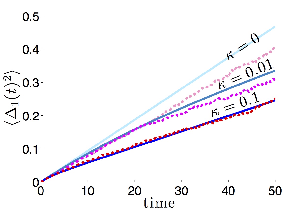
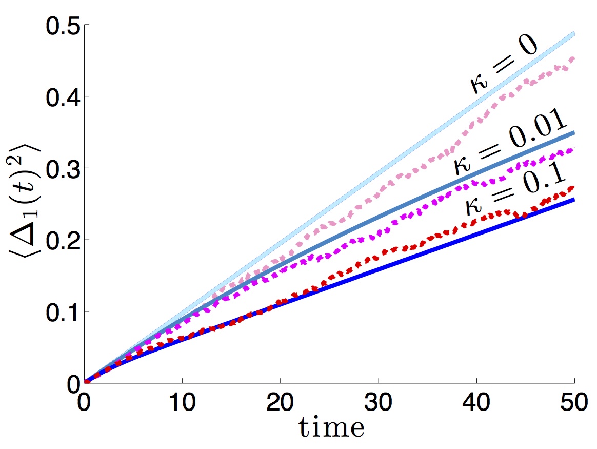
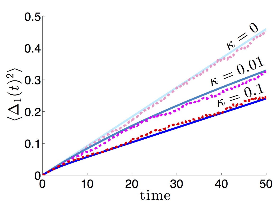
Figure 4: Effects of spatially homogeneous noise (Cj(x)=1subscript𝐶𝑗𝑥1C_{j}(x)=1) on propagation of coupled fronts. Theory (solid lines) given by (57) matches numerical simulations (dashed lines) reasonably well. As the strength of identical reciprocal coupling κ1=κ2=κsubscript𝜅1subscript𝜅2𝜅\kappa_{1}=\kappa_{2}=\kappa is increased, the variance of front position Δ1(t)2delimited-⟨⟩subscriptΔ1superscript𝑡2\langle\Delta_{1}(t)^{2}\rangle does not increase as quickly with time. Other parameters are θ=0.4𝜃0.4\theta=0.4 and ε=0.001𝜀0.001\varepsilon=0.001.
Refer to caption
Figure 5: Effects of cosine correlated noise (Cj(x)=cos(x)subscript𝐶𝑗𝑥𝑥C_{j}(x)=\cos(x)) on propagation of coupled fronts. Theory given by (58). As the strength of identical reciprocal coupling κ1=κ2=κsubscript𝜅1subscript𝜅2𝜅\kappa_{1}=\kappa_{2}=\kappa is increased, the variance of front position Δ1(t)2delimited-⟨⟩subscriptΔ1superscript𝑡2\langle\Delta_{1}(t)^{2}\rangle does not increase as quickly with time. Other parameters are θ=0.4𝜃0.4\theta=0.4 and ε=0.001𝜀0.001\varepsilon=0.001.
Refer to caption
Figure 6: Effects of exponentially correlated noise (Cj(x)=(1+|x|)e|x|subscript𝐶𝑗𝑥1𝑥superscripte𝑥C_{j}(x)=(1+|x|){\rm e}^{-|x|}) on propagation of coupled fronts. Theory given by (59). As the strength of identical reciprocal coupling κ1=κ2=κsubscript𝜅1subscript𝜅2𝜅\kappa_{1}=\kappa_{2}=\kappa is increased, the variance of front position Δ1(t)2delimited-⟨⟩subscriptΔ1superscript𝑡2\langle\Delta_{1}(t)^{2}\rangle does not increase as quickly with time. Other parameters are θ=0.4𝜃0.4\theta=0.4 and ε=0.001𝜀0.001\varepsilon=0.001.

For symmetric connections between areas, κ=ε1/2w¯12/(2θ)=ε1/2w¯21/(2θ)𝜅superscript𝜀12subscript¯𝑤122𝜃superscript𝜀12subscript¯𝑤212𝜃\kappa=\varepsilon^{1/2}\bar{w}_{12}/(2\theta)=\varepsilon^{1/2}\bar{w}_{21}/(2\theta), as well as identical noise, χ1=χ2=1subscript𝜒1subscript𝜒21\chi_{1}=\chi_{2}=1, we have Δ1(t)2=Δ2(t)2=Δ(t)2\langle\Delta_{1}(t)^{2}\rangle=\langle\Delta_{2}(t)^{2}=\langle\Delta(t)^{2}\rangle so that for effective coefficients D1=D2subscript𝐷1subscript𝐷2D_{1}=D_{2}, we have

Δ(t)2=Djt2+Dj8κ[1e4κt].delimited-⟨⟩Δsuperscript𝑡2subscript𝐷𝑗𝑡2subscript𝐷𝑗8𝜅delimited-[]1superscripte4𝜅𝑡\displaystyle\langle\Delta(t)^{2}\rangle=\frac{D_{j}t}{2}+\frac{D_{j}}{8\kappa}\left[1-{\rm e}^{-4\kappa t}\right]. (60)

We compare the formula (60) to results we obtain from numerical simulations in Figs. 4, 5, and 6.
Refer to caption
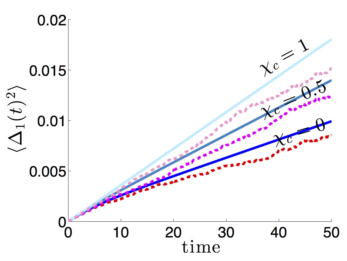
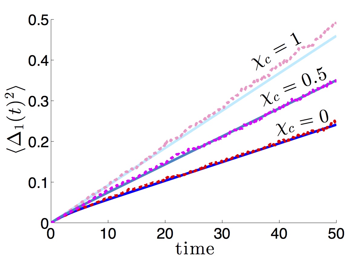
Figure 7: Effect of correlations between layers, for Cj(x)=cos(x)subscript𝐶𝑗𝑥𝑥C_{j}(x)=\cos(x) and Cc=χccos(x)subscript𝐶𝑐subscript𝜒𝑐𝑥C_{c}=\chi_{c}\cos(x), on the propagation of coupled fronts. As the amplitude of noise correlations between layers increases, the effect of reciprocal coupling κ1=κ2=0.1subscript𝜅1subscript𝜅20.1\kappa_{1}=\kappa_{2}=0.1 is reduced, as the the variance in front position Δ1(t)2delimited-⟨⟩subscriptΔ1superscript𝑡2\langle\Delta_{1}(t)^{2}\rangle scales more quickly all time. In the limit χc1subscript𝜒𝑐1\chi_{c}\to 1, the effects of reciprocal coupling on variance vanish. Other parameters are θ=0.4𝜃0.4\theta=0.4 and ε=0.001𝜀0.001\varepsilon=0.001.

In the case of correlations between layers, so χc>0subscript𝜒𝑐0\chi_{c}>0, meaning Dc>0subscript𝐷𝑐0D_{c}>0. In this case, the covariance terms in D+subscript𝐷D_{+} and Dsubscript𝐷D_{-} are non-zero. We can thus compute the diffusion coefficient associated with correlated noise in the case of cosine correlated noise

Dc=εχcσ24θ4(c2+σ2).subscript𝐷𝑐𝜀subscript𝜒𝑐superscript𝜎24superscript𝜃4superscript𝑐2superscript𝜎2\displaystyle D_{c}=\frac{\varepsilon\chi_{c}\sigma^{2}}{4\theta^{4}(c^{2}+\sigma^{2})}.

In the case of symmetric connections between layers and identical noise, we have Δ1=Δ2=ΔsubscriptΔ1subscriptΔ2Δ\Delta_{1}=\Delta_{2}=\Delta and for cosine correlated noise

Δ(t)2=(1+χc)σ2ε8θ4(c2+σ2)+(1χc)σ2ε32θ4(c2+σ2)κ[1e4κt],delimited-⟨⟩Δsuperscript𝑡21subscript𝜒𝑐superscript𝜎2𝜀8superscript𝜃4superscript𝑐2superscript𝜎21subscript𝜒𝑐superscript𝜎2𝜀32superscript𝜃4superscript𝑐2superscript𝜎2𝜅delimited-[]1superscripte4𝜅𝑡\displaystyle\langle\Delta(t)^{2}\rangle=\frac{(1+\chi_{c})\sigma^{2}\varepsilon}{8\theta^{4}(c^{2}+\sigma^{2})}+\frac{(1-\chi_{c})\sigma^{2}\varepsilon}{32\theta^{4}(c^{2}+\sigma^{2})\kappa}\left[1-{\rm e}^{-4\kappa t}\right], (61)

which shows interlaminar connections do not reduce variability as much when noise correlations between layers χcsubscript𝜒𝑐\chi_{c} are strong. We demonstrate the accuracy of the theoretical calculation (61) in comparison to numerical simulations in Fig. 7. Essentially, stronger noise correlations between layers diminish the effectiveness of interlaminar connections at reducing front position variance.

IV Dual ring network

IV.1 Coupled pulse propagation

We now study another common neural field model framework, asymmetric connectivity that produces traveling pulse solutions Xie and Giese (2002). To begin, we seek coupled traveling pulse solutions to (1) by constructing solutions in the traveling coordinate frame ξ=xct𝜉𝑥𝑐𝑡\xi=x-ct in the absence of noise (ε0𝜀0\varepsilon\to 0), where we will determine the wavespeed c𝑐c self-consistently. Note, this assumes that the pulses in each layer are locked to one another. We assume this baseline solution and study violations of this assumption as bifurcations from stable coupled traveling pulse solutions. Thus, we assume traveling wave solutions take the form (u1(x,t),u2(x,t))=(U1(ξ),U2(ξ))subscript𝑢1𝑥𝑡subscript𝑢2𝑥𝑡subscript𝑈1𝜉subscript𝑈2𝜉(u_{1}(x,t),u_{2}(x,t))=(U_{1}(\xi),U_{2}(\xi)). The translation invariance of the system allows us to set the leading edge of the first pulse to be at ξ=π𝜉𝜋\xi=\pi to ease calculations. The traveling pulse solutions then satisfy the system

cU1(ξ)𝑐superscriptsubscript𝑈1𝜉\displaystyle-cU_{1}^{\prime}(\xi) =U1(ξ)+w11f(U1)+w12f(U2),absentsubscript𝑈1𝜉subscript𝑤11𝑓subscript𝑈1subscript𝑤12𝑓subscript𝑈2\displaystyle=-U_{1}(\xi)+w_{11}*f(U_{1})+w_{12}*f(U_{2}), (62)
cU2(ξ)𝑐superscriptsubscript𝑈2𝜉\displaystyle-cU_{2}^{\prime}(\xi) =U2(ξ)+w22f(U2)+w21f(U1),absentsubscript𝑈2𝜉subscript𝑤22𝑓subscript𝑈2subscript𝑤21𝑓subscript𝑈1\displaystyle=-U_{2}(\xi)+w_{22}*f(U_{2})+w_{21}*f(U_{1}), (63)

where the convolution * is over Ω=[π,π]Ω𝜋𝜋\Omega=[-\pi,\pi] with the periodic boundary conditions Uj(π)=Uj(π)subscript𝑈𝑗𝜋subscript𝑈𝑗𝜋U_{j}(-\pi)=U_{j}(\pi) for j=1,2𝑗12j=1,2. As the system has been projected to a two dimensional set of ordinary differential equations, it can be solved using shooting methods for arbitrary choices of the nonlinearity f𝑓f Ermentrout and McLeod (1993); Pinto and Ermentrout (2001) to specify the wavespeed c𝑐c. For purposes of demonstration, we proceed assuming the nonlinearity is a Heaviside (8). Since we presume we are constructing coupled traveling pulse solutions, their profiles must cross above and below threshold, yielding the additional conditions U1(π)=U1(πa1)=U2(b)=U2(ba2)=θsubscript𝑈1𝜋subscript𝑈1𝜋subscript𝑎1subscript𝑈2𝑏subscript𝑈2𝑏subscript𝑎2𝜃U_{1}(\pi)=U_{1}(\pi-a_{1})=U_{2}(b)=U_{2}(b-a_{2})=\theta. Accounting for the periodicity of the functions U1subscript𝑈1U_{1} and U2subscript𝑈2U_{2} beyond domain [π,π]𝜋𝜋[-\pi,\pi], we note that if ba2<π𝑏subscript𝑎2𝜋b-a_{2}<-\pi, the last threshold condition will essentially ensure U(ba2+2π)=θ𝑈𝑏subscript𝑎22𝜋𝜃U(b-a_{2}+2\pi)=\theta. We can set the front crossing point of U1subscript𝑈1U_{1} to be at π𝜋\pi due to the underlying translation invariance of the system (1), which we will verify in our linear stability calculations. In addition, note that the leading edge of U2subscript𝑈2U_{2} and width a2subscript𝑎2a_{2} need not be the same as in U1subscript𝑈1U_{1}. Therefore, we have the equations (62) and (63) become

cU1(ξ)𝑐superscriptsubscript𝑈1𝜉\displaystyle-cU_{1}^{\prime}(\xi) =U1(ξ)+G1(ξ),absentsubscript𝑈1𝜉subscript𝐺1𝜉\displaystyle=-U_{1}(\xi)+G_{1}(\xi), (64)
cU2(ξ)𝑐superscriptsubscript𝑈2𝜉\displaystyle-cU_{2}^{\prime}(\xi) =U2(ξ)+G2(ξ),absentsubscript𝑈2𝜉subscript𝐺2𝜉\displaystyle=-U_{2}(\xi)+G_{2}(\xi), (65)

where

G1(x)subscript𝐺1𝑥\displaystyle G_{1}(x) =πaπw11(xy)dy+ba2bw12(xy)dyabsentsuperscriptsubscript𝜋𝑎𝜋subscript𝑤11𝑥𝑦differential-d𝑦superscriptsubscript𝑏subscript𝑎2𝑏subscript𝑤12𝑥𝑦differential-d𝑦\displaystyle=\int_{\pi-a}^{\pi}w_{11}(x-y){\rm d}y+\int_{b-a_{2}}^{b}w_{12}(x-y){\rm d}y
G2(x)subscript𝐺2𝑥\displaystyle G_{2}(x) =ba2bw22(xy)dy+πaπw21(xy)dy.absentsuperscriptsubscript𝑏subscript𝑎2𝑏subscript𝑤22𝑥𝑦differential-d𝑦superscriptsubscript𝜋𝑎𝜋subscript𝑤21𝑥𝑦differential-d𝑦\displaystyle=\int_{b-a_{2}}^{b}w_{22}(x-y){\rm d}y+\int_{\pi-a}^{\pi}w_{21}(x-y){\rm d}y.

Thus, we can integrate the two equations (64) and (65) and apply the threshold conditions U1(π)=θsubscript𝑈1𝜋𝜃U_{1}(\pi)=\theta and U2(b)=θsubscript𝑈2𝑏𝜃U_{2}(b)=\theta to yield

U1(ξ)subscript𝑈1𝜉\displaystyle U_{1}(\xi) =eξ/c(θeπ/c1cπξG1(y)ey/cdy)absentsuperscripte𝜉𝑐𝜃superscripte𝜋𝑐1𝑐superscriptsubscript𝜋𝜉subscript𝐺1𝑦superscripte𝑦𝑐differential-d𝑦\displaystyle={\rm e}^{\xi/c}\left(\theta{\rm e}^{-\pi/c}-\frac{1}{c}\int_{\pi}^{\xi}G_{1}(y){\rm e}^{-y/c}{\rm d}y\right) (66)
U2(ξ)subscript𝑈2𝜉\displaystyle U_{2}(\xi) =eξ/c(θeb/c1cbξG2(y)ey/cdy).absentsuperscripte𝜉𝑐𝜃superscripte𝑏𝑐1𝑐superscriptsubscript𝑏𝜉subscript𝐺2𝑦superscripte𝑦𝑐differential-d𝑦\displaystyle={\rm e}^{\xi/c}\left(\theta{\rm e}^{-b/c}-\frac{1}{c}\int_{b}^{\xi}G_{2}(y){\rm e}^{-y/c}{\rm d}y\right). (67)

By requiring that periodicity holds, Uj(π)=Uj(π)subscript𝑈𝑗𝜋subscript𝑈𝑗𝜋U_{j}(-\pi)=U_{j}(\pi) for j=1,2𝑗12j=1,2, we have

2cθsinhπc2𝑐𝜃𝜋𝑐\displaystyle 2c\theta\sinh\frac{\pi}{c} =ππG1(y)ey/cdyabsentsuperscriptsubscript𝜋𝜋subscript𝐺1𝑦superscripte𝑦𝑐differential-d𝑦\displaystyle=\int_{-\pi}^{\pi}G_{1}(y){\rm e}^{-y/c}{\rm d}y
2cθeb/csinhπc2𝑐𝜃superscripte𝑏𝑐𝜋𝑐\displaystyle 2c\theta{\rm e}^{-b/c}\sinh\frac{\pi}{c} =eπ/cbπG2(y)ey/cdyabsentsuperscripte𝜋𝑐superscriptsubscript𝑏𝜋subscript𝐺2𝑦superscripte𝑦𝑐differential-d𝑦\displaystyle={\rm e}^{\pi/c}\int_{b}^{\pi}G_{2}(y){\rm e}^{-y/c}{\rm d}y
eπ/cbπG2(y)ey/cdysuperscripte𝜋𝑐superscriptsubscript𝑏𝜋subscript𝐺2𝑦superscripte𝑦𝑐differential-d𝑦\displaystyle-{\rm e}^{-\pi/c}\int_{b}^{-\pi}G_{2}(y){\rm e}^{-y/c}{\rm d}y

Now, we can generate implicit expressions for the wavespeed c𝑐c, widths a1subscript𝑎1a_{1} and a2subscript𝑎2a_{2}, and the position b𝑏b by applying the remaining threshold conditions U1(πa1)=θsubscript𝑈1𝜋subscript𝑎1𝜃U_{1}(\pi-a_{1})=\theta and U2(g(a2))=θsubscript𝑈2𝑔subscript𝑎2𝜃U_{2}(g(a_{2}))=\theta we have

cθ(e(a1π)/ceπ/c)𝑐𝜃superscriptesubscript𝑎1𝜋𝑐superscripte𝜋𝑐\displaystyle c\theta({\rm e}^{(a_{1}-\pi)/c}-{\rm e}^{-\pi/c}) =πa1πG1(y)ey/cdy,absentsuperscriptsubscript𝜋subscript𝑎1𝜋subscript𝐺1𝑦superscripte𝑦𝑐differential-d𝑦\displaystyle=\int_{\pi-a_{1}}^{\pi}G_{1}(y){\rm e}^{-y/c}{\rm d}y,
cθ(e(a2b)/ceb/c)𝑐𝜃superscriptesubscript𝑎2𝑏𝑐superscripte𝑏𝑐\displaystyle c\theta({\rm e}^{(a_{2}-b)/c}-{\rm e}^{-b/c}) =ba2bG2(y)ey/cdy,absentsuperscriptsubscript𝑏subscript𝑎2𝑏subscript𝐺2𝑦superscripte𝑦𝑐differential-d𝑦\displaystyle=\int_{b-a_{2}}^{b}G_{2}(y){\rm e}^{-y/c}{\rm d}y,

which can be solved using numerical root finding for a general choice of wjksubscript𝑤𝑗𝑘w_{jk} (j,k=1,2formulae-sequence𝑗𝑘12j,k=1,2).

Refer to caption
Figure 8: A Speed c𝑐c and B position parameter b𝑏b of coupled traveling pulses (66) and (67) as determined by the implicit system (68) in the a case of asymmetric reciprocal connectivity w¯12w¯21subscript¯𝑤12subscript¯𝑤21\bar{w}_{12}\neq\bar{w}_{21}, in general. Other parameters w¯12=0.1subscript¯𝑤120.1\bar{w}_{12}=0.1, ϕ=π/8italic-ϕ𝜋8\phi=\pi/8, and θ=0.4𝜃0.4\theta=0.4.
Refer to caption
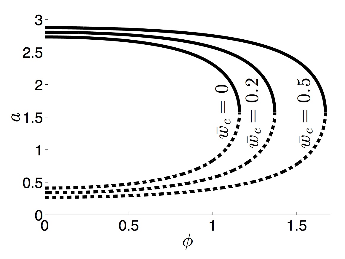
Figure 9: Pulsewidth a1=a2=asubscript𝑎1subscript𝑎2𝑎a_{1}=a_{2}=a as a function of the asymmetry ϕitalic-ϕ\phi of the local weight functions w1(x)=w2(x)=cos(xϕ)subscript𝑤1𝑥subscript𝑤2𝑥𝑥italic-ϕw_{1}(x)=w_{2}(x)=\cos(x-\phi) for varying amplitudes of reciprocal symmetric strength w¯12=w¯21=w¯csubscript¯𝑤12subscript¯𝑤21subscript¯𝑤𝑐\bar{w}_{12}=\bar{w}_{21}=\bar{w}_{c}. Increasing the strength w¯csubscript¯𝑤𝑐\bar{w}_{c} shifts the saddle-node bifurcation, at which the stable (solid) and unstable (dashed) branches of pulse solutions, to the right in ϕitalic-ϕ\phi. Other parameter θ=0.4𝜃0.4\theta=0.4.

We can compute these expressions in the case where the weight functions are specified by (3) and (4), so that

θ𝜃\displaystyle\theta =𝒫(a1)+w¯12𝒬(a2,b)c2+1,absent𝒫subscript𝑎1subscript¯𝑤12𝒬subscript𝑎2𝑏superscript𝑐21\displaystyle=\frac{{\mathcal{P}}(a_{1})+\bar{w}_{12}{\mathcal{Q}}(a_{2},b)}{c^{2}+1}, (68)
θ𝜃\displaystyle\theta =(a1)+w¯12𝒮(a1,a2,b)c2+1,absentsubscript𝑎1subscript¯𝑤12𝒮subscript𝑎1subscript𝑎2𝑏superscript𝑐21\displaystyle=\frac{{\mathcal{R}}(a_{1})+\bar{w}_{12}{\mathcal{S}}(a_{1},a_{2},b)}{c^{2}+1},
θ𝜃\displaystyle\theta =𝒫(a2)+w¯21𝒬(a1,b)c2+1,absent𝒫subscript𝑎2subscript¯𝑤21𝒬subscript𝑎1𝑏superscript𝑐21\displaystyle=\frac{{\mathcal{P}}(a_{2})+\bar{w}_{21}{\mathcal{Q}}(a_{1},-b)}{c^{2}+1},
θ𝜃\displaystyle\theta =(a2)+w¯21𝒮(a2,a1,b)c2+1,absentsubscript𝑎2subscript¯𝑤21𝒮subscript𝑎2subscript𝑎1𝑏superscript𝑐21\displaystyle=\frac{{\mathcal{R}}(a_{2})+\bar{w}_{21}{\mathcal{S}}(a_{2},a_{1},-b)}{c^{2}+1},

where

𝒫(x)𝒫𝑥\displaystyle{\mathcal{P}}(x) =sinϕccosϕ+ccos(xϕ)sin(ϕx),absentitalic-ϕ𝑐italic-ϕ𝑐𝑥italic-ϕitalic-ϕ𝑥\displaystyle=\sin\phi-c\cos\phi+c\cos(x-\phi)-\sin(\phi-x),
𝒬(x,y)𝒬𝑥𝑦\displaystyle{\mathcal{Q}}(x,y) =sin(yx)+ccosysinyccos(xy),absent𝑦𝑥𝑐𝑦𝑦𝑐𝑥𝑦\displaystyle=\sin(y-x)+c\cos y-\sin y-c\cos(x-y),
(x)𝑥\displaystyle{\mathcal{R}}(x) =sin(x+ϕ)sinϕ+ccosϕccos(x+ϕ),absent𝑥italic-ϕitalic-ϕ𝑐italic-ϕ𝑐𝑥italic-ϕ\displaystyle=\sin(x+\phi)-\sin\phi+c\cos\phi-c\cos(x+\phi),
𝒮(x,y,z)𝒮𝑥𝑦𝑧\displaystyle{\mathcal{S}}(x,y,z) =ccos(x+z)+sin(xy+z)absent𝑐𝑥𝑧𝑥𝑦𝑧\displaystyle=c\cos(x+z)+\sin(x-y+z)
sin(x+z)ccos(xy+z).𝑥𝑧𝑐𝑥𝑦𝑧\displaystyle-\sin(x+z)-c\cos(x-y+z).

We can solve the system of equations (68) numerically to show the effects of varying the coupling w¯12subscript¯𝑤12\bar{w}_{12} while keeping w¯21subscript¯𝑤21\bar{w}_{21} fixed. As shown in Fig. 8, increasing the strength w¯12subscript¯𝑤12\bar{w}_{12} leads to a decrease in wave speed c𝑐c and a decrease in the position b𝑏b of the second pulse. In the case of symmetric connectivity w¯12=w¯21=w¯csubscript¯𝑤12subscript¯𝑤21subscript¯𝑤𝑐\bar{w}_{12}=\bar{w}_{21}=\bar{w}_{c}, the system will simplify to a single equation, specifying the symmetric front solution U1(ξ)=U2(ξ)subscript𝑈1𝜉subscript𝑈2𝜉U_{1}(\xi)=U_{2}(\xi). Thus, b=π𝑏𝜋b=\pi and a1=a2=asubscript𝑎1subscript𝑎2𝑎a_{1}=a_{2}=a, and we can simplify the system to

θ𝜃\displaystyle\theta =[cosϕ+csinϕ+w¯c]sinac2+1,absentdelimited-[]italic-ϕ𝑐italic-ϕsubscript¯𝑤𝑐𝑎superscript𝑐21\displaystyle=\frac{[\cos\phi+c\sin\phi+\bar{w}_{c}]\sin a}{c^{2}+1}, (69)
00\displaystyle 0 =(1cosa)(sinϕccosϕcw¯c)c2+1.absent1𝑎italic-ϕ𝑐italic-ϕ𝑐subscript¯𝑤𝑐superscript𝑐21\displaystyle=\frac{(1-\cos a)(\sin\phi-c\cos\phi-c\bar{w}_{c})}{c^{2}+1}. (70)

We can exclude the solution cosa=1𝑎1\cos a=1 to (70), since this will not solve the other equations. Thus, we use the other solution to (70) to find that

c=sinϕcosϕ+w¯c𝑐italic-ϕitalic-ϕsubscript¯𝑤𝑐\displaystyle c=\frac{\sin\phi}{\cos\phi+\bar{w}_{c}}

will be the wave speed. Thus, as opposed to the case of coupled traveling fronts, strengthening connectivity w¯csubscript¯𝑤𝑐\bar{w}_{c} here decreases the wave speed. Plugging this into (69), we find that sina=θ/cosϕ+w¯c𝑎𝜃italic-ϕsubscript¯𝑤𝑐\sin a=\theta/\cos\phi+\bar{w}_{c}, so

assubscript𝑎𝑠\displaystyle a_{s} =πsin1θcosϕ+w¯c,absent𝜋superscript1𝜃italic-ϕsubscript¯𝑤𝑐\displaystyle=\pi-\sin^{-1}\frac{\theta}{\cos\phi+\bar{w}_{c}}, (71)
ausubscript𝑎𝑢\displaystyle a_{u} =sin1θcosϕ+w¯cabsentsuperscript1𝜃italic-ϕsubscript¯𝑤𝑐\displaystyle=\sin^{-1}\frac{\theta}{\cos\phi+\bar{w}_{c}} (72)

defines the widths of a coexistent pair of stable (71) and unstable (72) coupled traveling pulse solutions. Note that these two branches will coalesce in a saddle-node bifurcation (see Kilpatrick and Ermentrout (2012) for analysis in a single layer network). This bifurcation point is determined by where θ=cosϕ+w¯c𝜃italic-ϕsubscript¯𝑤𝑐\theta=\cos\phi+\bar{w}_{c}, as shown in Fig. 9.

In the limit w¯c0subscript¯𝑤𝑐0\bar{w}_{c}\to 0, the pulses are decoupled, both then having speed c=tanϕ𝑐italic-ϕc=\tan\phi. Pulses will then be neutrally stable to perturbations in both directions. This can be seen by using the same analysis we performed for the excitatory neuronal network that supported fronts. Essentially, perturbations must obey (20), which has an eigenvalue λ=0𝜆0\lambda=0 associated with the eigenfunction Ujsuperscriptsubscript𝑈𝑗U_{j}^{\prime} for each layer j=1,2𝑗12j=1,2. We will now show that coupling layers stabilizes pulses to perturbations that pull them in opposite directions.

IV.2 Noise-induced motion of coupled pulses

Now, we analyze the effects of weak noise on the propagation of pulses in the presence of reciprocal coupling that is weak (w12,w21=𝒪(ε1/2)subscript𝑤12subscript𝑤21𝒪superscript𝜀12w_{12},w_{21}={\mathcal{O}}(\varepsilon^{1/2})) and local coupling that is identical (w11=w22=wsubscript𝑤11subscript𝑤22𝑤w_{11}=w_{22}=w). To start, we presume noise causes each pulse’s position to wander, described by stochastic variables Δ1(t)subscriptΔ1𝑡\Delta_{1}(t) and Δ2(t)subscriptΔ2𝑡\Delta_{2}(t), and each pulse’s profile fluctuates, described by the stochastic variables Φ1(x,t)subscriptΦ1𝑥𝑡\Phi_{1}(x,t) and Φ2(x,t)subscriptΦ2𝑥𝑡\Phi_{2}(x,t). As in the case of coupled traveling fronts, this is described by the expansion given by the ansatz (22). Plugging this into (1) and expanding in powers of ε1/2superscript𝜀12\varepsilon^{1/2}, we find the pulse solution at 𝒪(1)𝒪1{\mathcal{O}}(1) where w¯12=w¯210subscript¯𝑤12subscript¯𝑤210\bar{w}_{12}=\bar{w}_{21}\equiv 0. At 𝒪(ε1/2)𝒪superscript𝜀12{\mathcal{O}}(\varepsilon^{1/2}), we find the system (25) with associated linear operator {\mathcal{L}}, as we found for the excitatory network with fronts. Again, we find that the null space of {\mathcal{L}} includes the vectors (U1,0)Tsuperscriptsuperscriptsubscript𝑈10𝑇(U_{1}^{\prime},0)^{T} and (0,U2)Tsuperscript0superscriptsubscript𝑈2𝑇(0,U_{2}^{\prime})^{T} due to equation (20). Next, we apply a solvability condition to (25), where the inhomogenous part must be orthogonal to the nullspace of

𝐩=(cp(x)p(x)+f(U1)[w(x)p(x)]cq(x)q(x)+f(U2)[w(x)q(x)])superscript𝐩𝑐superscript𝑝𝑥𝑝𝑥superscript𝑓subscript𝑈1delimited-[]𝑤𝑥𝑝𝑥𝑐superscript𝑞𝑥𝑞𝑥superscript𝑓subscript𝑈2delimited-[]𝑤𝑥𝑞𝑥\displaystyle{\mathcal{L}}^{*}{\mathbf{p}}=\left(\begin{array}[]{c}-cp^{\prime}(x)-p(x)+f^{\prime}(U_{1})[w(-x)*p(x)]\\ -cq^{\prime}(x)-q(x)+f^{\prime}(U_{2})[w(-x)*q(x)]\end{array}\right) (75)

where p=(p(x),q(x))T𝑝superscript𝑝𝑥𝑞𝑥𝑇p=(p(x),q(x))^{T}. It is important to note that an asymmetric weight function w(x)𝑤𝑥w(x), like (3), leads to a slightly different form for superscript{\mathcal{L}}^{*}, now involving terms like w(x)p(x)=ππw(yx)p(y)dy𝑤𝑥𝑝𝑥superscriptsubscript𝜋𝜋𝑤𝑦𝑥𝑝𝑦differential-d𝑦w(-x)*p(x)=\int_{-\pi}^{\pi}w(y-x)p(y){\rm d}y. Again, we can decomposed the nullspace of superscript{\mathcal{L}}^{*} into two orthogonal elements that take the forms (φ1,0)Tsuperscriptsubscript𝜑10𝑇(\varphi_{1},0)^{T} and (0,φ2)Tsuperscript0subscript𝜑2𝑇(0,\varphi_{2})^{T}. Rearranging the resulting solvability condition shows that the stochastic vector 𝚫(t)=(Δ1(t),Δ2(t))T𝚫𝑡superscriptsubscriptΔ1𝑡subscriptΔ2𝑡𝑇{\mathbf{\Delta}}(t)=(\Delta_{1}(t),\Delta_{2}(t))^{T} obeys the multivariate Ornstein-Uhlenbeck process

d𝚫(t)=[𝐉+𝐊𝚫(t)]dt+d𝐖(t)d𝚫𝑡delimited-[]𝐉𝐊𝚫𝑡d𝑡d𝐖𝑡\displaystyle{\rm d}{\mathbf{\Delta}}(t)=\left[{\mathbf{J}}+{\mathbf{K}}{\mathbf{\Delta}}(t)\right]{\rm d}t+{\rm d}{\mathbf{W}}(t) (76)

where connections between the two layers will slightly alter the mean speed through the term

𝐉=(γ1γ2)=(φ1,ε1/2w12f(U2)φ1,U1φ2,ε1/2w21f(U1)φ2,U2)𝐉subscript𝛾1subscript𝛾2subscript𝜑1superscript𝜀12subscript𝑤12𝑓subscript𝑈2subscript𝜑1superscriptsubscript𝑈1subscript𝜑2superscript𝜀12subscript𝑤21𝑓subscript𝑈1subscript𝜑2superscriptsubscript𝑈2\displaystyle{\mathbf{J}}=\left(\begin{array}[]{c}\gamma_{1}\\ \gamma_{2}\end{array}\right)=\left(\begin{array}[]{c}-\frac{\displaystyle\langle\varphi_{1},\varepsilon^{1/2}w_{12}*f(U_{2})\rangle}{\displaystyle\langle\varphi_{1},U_{1}^{\prime}\rangle}\\ -\frac{\displaystyle\langle\varphi_{2},\varepsilon^{1/2}w_{21}*f(U_{1})\rangle}{\displaystyle\langle\varphi_{2},U_{2}^{\prime}\rangle}\end{array}\right) (81)

and pull the positions of both fronts to one another according to the coupling matrix

𝐊=(κ1κ1κ2κ2),𝐊subscript𝜅1subscript𝜅1subscript𝜅2subscript𝜅2\displaystyle{\mathbf{K}}=\left(\begin{array}[]{cc}-\kappa_{1}&\kappa_{1}\\ \kappa_{2}&-\kappa_{2}\end{array}\right),

with

κ1subscript𝜅1\displaystyle\kappa_{1} =φ1,ε1/2w12[f(U2)U2]φ1,U1,absentsubscript𝜑1superscript𝜀12subscript𝑤12delimited-[]superscript𝑓subscript𝑈2superscriptsubscript𝑈2subscript𝜑1superscriptsubscript𝑈1\displaystyle=\frac{\langle\varphi_{1},\varepsilon^{1/2}w_{12}*[f^{\prime}(U_{2})U_{2}^{\prime}]\rangle}{\langle\varphi_{1},U_{1}^{\prime}\rangle},
κ2subscript𝜅2\displaystyle\kappa_{2} =φ2,ε1/2w21[f(U1)U1]φ2,U2,absentsubscript𝜑2superscript𝜀12subscript𝑤21delimited-[]superscript𝑓subscript𝑈1superscriptsubscript𝑈1subscript𝜑2superscriptsubscript𝑈2\displaystyle=\frac{\langle\varphi_{2},\varepsilon^{1/2}w_{21}*[f^{\prime}(U_{1})U_{1}^{\prime}]\rangle}{\langle\varphi_{2},U_{2}^{\prime}\rangle},

defining the inner product u,v=ππu(x)v(x)dx𝑢𝑣superscriptsubscript𝜋𝜋𝑢𝑥𝑣𝑥differential-d𝑥\langle u,v\rangle=\int_{-\pi}^{\pi}u(x)v(x){\rm d}x. Noise is described by the vector d𝐖(t)=(d𝒲1,d𝒲2)Td𝐖𝑡superscriptdsubscript𝒲1dsubscript𝒲2𝑇{\rm d}{\mathbf{W}}(t)=({\rm d}{\mathcal{W}}_{1},{\rm d}{\mathcal{W}}_{2})^{T} with

d𝒲j=ε1/2φj,dWjφj,Uj,j=1,2,formulae-sequencedsubscript𝒲𝑗superscript𝜀12subscript𝜑𝑗dsubscript𝑊𝑗subscript𝜑𝑗superscriptsubscript𝑈𝑗𝑗12\displaystyle{\rm d}{\mathcal{W}}_{j}=-\varepsilon^{1/2}\frac{\langle\varphi_{j},{\rm d}W_{j}\rangle}{\langle\varphi_{j},U_{j}^{\prime}\rangle},\ \ \ \ j=1,2,

with mean 𝐖(t)=𝟎delimited-⟨⟩𝐖𝑡0\langle{\mathbf{W}}(t)\rangle={\mathbf{0}}, variance 𝐖(t)𝐖T(t)=𝐃tdelimited-⟨⟩𝐖𝑡superscript𝐖𝑇𝑡𝐃𝑡\langle{\mathbf{W}}(t){\mathbf{W}}^{T}(t)\rangle={\mathbf{D}}t, and

𝐃=(D1DcDcD2)𝐃subscript𝐷1subscript𝐷𝑐subscript𝐷𝑐subscript𝐷2\displaystyle{\mathbf{D}}=\left(\begin{array}[]{cc}D_{1}&D_{c}\\ D_{c}&D_{2}\end{array}\right)

with diffusion coefficients

Dj=εππππφj(x)φj(y)Cj(xy)dxdy[ππφj(x)Uj(x)dx]2,j=1,2,formulae-sequencesubscript𝐷𝑗𝜀superscriptsubscript𝜋𝜋superscriptsubscript𝜋𝜋subscript𝜑𝑗𝑥subscript𝜑𝑗𝑦subscript𝐶𝑗𝑥𝑦differential-d𝑥differential-d𝑦superscriptdelimited-[]superscriptsubscript𝜋𝜋subscript𝜑𝑗𝑥superscriptsubscript𝑈𝑗𝑥differential-d𝑥2𝑗12\displaystyle D_{j}=\varepsilon\frac{\int_{-\pi}^{\pi}\int_{-\pi}^{\pi}\varphi_{j}(x)\varphi_{j}(y)C_{j}(x-y){\rm d}x{\rm d}y}{\left[\int_{-\pi}^{\pi}\varphi_{j}(x)U_{j}^{\prime}(x){\rm d}x\right]^{2}},\ \ \ j=1,2,

and covariance described by the coefficient

Dc=εππππφ1(x)φ2(y)Cc(xy)dxdy[ππφ1(x)U1(x)dx][ππφ2(x)U2(x)dx].subscript𝐷𝑐𝜀superscriptsubscript𝜋𝜋superscriptsubscript𝜋𝜋subscript𝜑1𝑥subscript𝜑2𝑦subscript𝐶𝑐𝑥𝑦differential-d𝑥differential-d𝑦delimited-[]superscriptsubscript𝜋𝜋subscript𝜑1𝑥superscriptsubscript𝑈1𝑥differential-d𝑥delimited-[]superscriptsubscript𝜋𝜋subscript𝜑2𝑥superscriptsubscript𝑈2𝑥differential-d𝑥\displaystyle D_{c}=\varepsilon\frac{\int_{-\pi}^{\pi}\int_{-\pi}^{\pi}\varphi_{1}(x)\varphi_{2}(y)C_{c}(x-y){\rm d}x{\rm d}y}{\left[\int_{-\pi}^{\pi}\varphi_{1}(x)U_{1}^{\prime}(x){\rm d}x\right]\left[\int_{-\pi}^{\pi}\varphi_{2}(x)U_{2}^{\prime}(x){\rm d}x\right]}.

As before, we can diagonalize the system to compute the covariance matrix 𝚫(t)𝚫(t)Tdelimited-⟨⟩𝚫𝑡𝚫superscript𝑡𝑇\langle{\mathbf{\Delta}}(t){\mathbf{\Delta}}(t)^{T}\rangle, and we are mainly interested in

Δ1(t)2delimited-⟨⟩subscriptΔ1superscript𝑡2\displaystyle\langle\Delta_{1}(t)^{2}\rangle =D+t+2κ1r1(t)+κ1κ2r2(t)absentsubscript𝐷𝑡2subscript𝜅1subscript𝑟1𝑡subscript𝜅1subscript𝜅2subscript𝑟2𝑡\displaystyle=D_{+}t+2\kappa_{1}r_{1}(t)+\frac{\kappa_{1}}{\kappa_{2}}r_{2}(t) (82)
Δ2(t)2delimited-⟨⟩subscriptΔ2superscript𝑡2\displaystyle\langle\Delta_{2}(t)^{2}\rangle =D+t2κ2r1(t)+κ2κ1r2(t)absentsubscript𝐷𝑡2subscript𝜅2subscript𝑟1𝑡subscript𝜅2subscript𝜅1subscript𝑟2𝑡\displaystyle=D_{+}t-2\kappa_{2}r_{1}(t)+\frac{\kappa_{2}}{\kappa_{1}}r_{2}(t) (83)

since these give the variance in the positions Δ1subscriptΔ1\Delta_{1} and Δ2subscriptΔ2\Delta_{2} of each pulse, which may encode temporal or spatial information. Again, the effective diffusion coefficients are

D+subscript𝐷\displaystyle D_{+} =κ22D1+2κ1κ2Dc+κ12D2(κ1+κ2)2absentsuperscriptsubscript𝜅22subscript𝐷12subscript𝜅1subscript𝜅2subscript𝐷𝑐superscriptsubscript𝜅12subscript𝐷2superscriptsubscript𝜅1subscript𝜅22\displaystyle=\frac{\kappa_{2}^{2}D_{1}+2\kappa_{1}\kappa_{2}D_{c}+\kappa_{1}^{2}D_{2}}{(\kappa_{1}+\kappa_{2})^{2}}
Drsubscript𝐷𝑟\displaystyle D_{r} =κ2D1κ1D2+(κ1κ2)Dc(κ1+κ2)2absentsubscript𝜅2subscript𝐷1subscript𝜅1subscript𝐷2subscript𝜅1subscript𝜅2subscript𝐷𝑐superscriptsubscript𝜅1subscript𝜅22\displaystyle=\frac{\kappa_{2}D_{1}-\kappa_{1}D_{2}+(\kappa_{1}-\kappa_{2})D_{c}}{(\kappa_{1}+\kappa_{2})^{2}}
Dsubscript𝐷\displaystyle D_{-} =D12Dc+D2(κ1+κ2)2absentsubscript𝐷12subscript𝐷𝑐subscript𝐷2superscriptsubscript𝜅1subscript𝜅22\displaystyle=\frac{D_{1}-2D_{c}+D_{2}}{(\kappa_{1}+\kappa_{2})^{2}}

and

r1(t)subscript𝑟1𝑡\displaystyle r_{1}(t) =Drκ1+κ2[1e(κ1+κ2)t],absentsubscript𝐷𝑟subscript𝜅1subscript𝜅2delimited-[]1superscriptesubscript𝜅1subscript𝜅2𝑡\displaystyle=\frac{D_{r}}{\kappa_{1}+\kappa_{2}}\left[1-{\rm e}^{-(\kappa_{1}+\kappa_{2})t}\right],
r2(t)subscript𝑟2𝑡\displaystyle r_{2}(t) =κ1κ2D2(κ1+κ2)[1e2(κ1+κ2)t].absentsubscript𝜅1subscript𝜅2subscript𝐷2subscript𝜅1subscript𝜅2delimited-[]1superscripte2subscript𝜅1subscript𝜅2𝑡\displaystyle=\frac{\kappa_{1}\kappa_{2}D_{-}}{2(\kappa_{1}+\kappa_{2})}\left[1-{\rm e}^{-2(\kappa_{1}+\kappa_{2})t}\right].

As in the excitatory network with fronts, we can note that the long term effective diffusion of both Δ1subscriptΔ1\Delta_{1} an Δ2subscriptΔ2\Delta_{2} is D+subscript𝐷D_{+}, and in the case of a symmetric network, variances will be identical and given by (46). Therefore, the main differences will arise in how the particular weight functions (3) and (4) as well as the shape of the traveling pulses (66) and (67) affects the transfer of noise between layers.

IV.3 Calculating stochastic motion of coupled pulses

Now, we will compute the variances (82) and (83) considering the specific case of Heaviside firing rate functions (8) and cosine synaptic weights (3) and (4). In particular, we will take w11=w22subscript𝑤11subscript𝑤22w_{11}=w_{22} to compare our asymptotic results to numerical simulations. To compute the pulse speed corrections γ1subscript𝛾1\gamma_{1} and γ2subscript𝛾2\gamma_{2}, we must first calculate the pulse solutions of the decoupled system Xie and Giese (2002); Kilpatrick and Ermentrout (2012)

Uj(ξ)=cosϕ(sinξsin(ξ+a))subscript𝑈𝑗𝜉italic-ϕ𝜉𝜉𝑎\displaystyle U_{j}(\xi)=\cos\phi(\sin\xi-\sin(\xi+a)) (84)

where a=πsin1[θsecϕ]𝑎𝜋superscript1𝜃italic-ϕa=\pi-\sin^{-1}[\theta\sec\phi] for the stable pulse. The spatial derivatives

Uj(ξ)=cosϕ(cosξcos(ξ+a)).superscriptsubscript𝑈𝑗𝜉italic-ϕ𝜉𝜉𝑎\displaystyle U_{j}^{\prime}(\xi)=\cos\phi(\cos\xi-\cos(\xi+a)). (85)

We can now solve explicitly for the null-vectors of superscript{\mathcal{L}}^{*}. Plugging (84) and (85) into (75) to find the each of the two equations in the vector system 𝝋=𝟎superscript𝝋0{\mathcal{L}}^{*}{\boldsymbol{\varphi}}={\mathbf{0}} is

cdφjdξ+φj𝑐dsubscript𝜑𝑗d𝜉subscript𝜑𝑗\displaystyle c\frac{{\rm d}\varphi_{j}}{{\rm d}\xi}+\varphi_{j} =C(π)δ(ξ+π)+C(πa)δ(ξπ+a)absent𝐶𝜋𝛿𝜉𝜋𝐶𝜋𝑎𝛿𝜉𝜋𝑎\displaystyle=C(-\pi)\delta(\xi+\pi)+C(\pi-a)\delta(\xi-\pi+a) (86)
C(ξ)𝐶𝜉\displaystyle C(\xi) =ππcos(yξϕ)φj(y)dy|cosϕ|[1cosa].absentsuperscriptsubscript𝜋𝜋𝑦𝜉italic-ϕsubscript𝜑𝑗𝑦differential-d𝑦italic-ϕdelimited-[]1𝑎\displaystyle=\frac{\displaystyle\int_{-\pi}^{\pi}\cos(y-\xi-\phi)\varphi_{j}(y){\rm d}y}{\displaystyle|\cos\phi|[1-\cos a]}.

Using the 2π2𝜋2\pi periodicity along with a self-consistency argument, we can solve (86) explicitly to yield Kilpatrick and Ermentrout (2012)

φj(ξ)subscript𝜑𝑗𝜉\displaystyle\varphi_{j}(\xi) =[H(ξ+π)+coth(π/c)12]e(π+ξ)/cabsentdelimited-[]𝐻𝜉𝜋hyperbolic-cotangent𝜋𝑐12superscripte𝜋𝜉𝑐\displaystyle=\left[H(\xi+\pi)+\frac{\coth(\pi/c)-1}{2}\right]{\rm e}^{-(\pi+\xi)/c}
[H(ξ+aπ)+coth(π/c)12]e(πaξ)/c.delimited-[]𝐻𝜉𝑎𝜋hyperbolic-cotangent𝜋𝑐12superscripte𝜋𝑎𝜉𝑐\displaystyle-\left[H(\xi+a-\pi)+\frac{\coth(\pi/c)-1}{2}\right]{\rm e}^{(\pi-a-\xi)/c}.

We can then evaluate the integrals in (81) to yield

γ1=ε1/2w¯12ccosϕ,γ2=ε1/2w¯21ccosϕ,formulae-sequencesubscript𝛾1superscript𝜀12subscript¯𝑤12𝑐italic-ϕsubscript𝛾2superscript𝜀12subscript¯𝑤21𝑐italic-ϕ\displaystyle\gamma_{1}=-\frac{\varepsilon^{1/2}\bar{w}_{12}c}{\cos\phi},\ \ \ \ \ \gamma_{2}=-\frac{\varepsilon^{1/2}\bar{w}_{21}c}{\cos\phi},

so as predicted by our nonlinear analysis, the pulses will slow down as the strength of inter-laminar connectivity w¯jksubscript¯𝑤𝑗𝑘\bar{w}_{jk} is increased. To compute the coupling strengths κ1subscript𝜅1\kappa_{1} and κ2subscript𝜅2\kappa_{2}, we must also compute

f(Uj)Uj=δ(ξ+aπ)δ(ξπ),superscript𝑓subscript𝑈𝑗superscriptsubscript𝑈𝑗𝛿𝜉𝑎𝜋𝛿𝜉𝜋\displaystyle f^{\prime}(U_{j})U_{j}^{\prime}=\delta(\xi+a-\pi)-\delta(\xi-\pi),

in the sense of distributions, so that the coupling terms are given
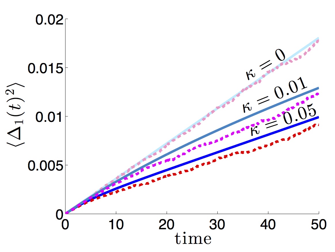
κ1=ε1/2w¯12cosϕ,κ2=ε1/2w¯21cosϕ.formulae-sequencesubscript𝜅1superscript𝜀12subscript¯𝑤12italic-ϕsubscript𝜅2superscript𝜀12subscript¯𝑤21italic-ϕ\displaystyle\kappa_{1}=\frac{\varepsilon^{1/2}\bar{w}_{12}}{\cos\phi},\ \ \ \ \ \ \ \kappa_{2}=\frac{\varepsilon^{1/2}\bar{w}_{21}}{\cos\phi}.
Refer to caption
Figure 10: Effects of cosine correlated noise (Cj(x)=cos(x)subscript𝐶𝑗𝑥𝑥C_{j}(x)=\cos(x)) on propagation of coupled pulses. As the strength of identical reciprocal coupling κ1=κ2=κsubscript𝜅1subscript𝜅2𝜅\kappa_{1}=\kappa_{2}=\kappa is increased, the variance of pulse position Δ1(t)2delimited-⟨⟩subscriptΔ1superscript𝑡2\langle\Delta_{1}(t)^{2}\rangle does not increase as quickly with time. Other parameters are θ=0.4𝜃0.4\theta=0.4 and ε=0.001𝜀0.001\varepsilon=0.001.
Refer to caption
Figure 11: Effects of cosine correlated noise (Cj(x)=cos(x)subscript𝐶𝑗𝑥𝑥C_{j}(x)=\cos(x)) on propagation of coupled pulses when there are noise-correlations between layers (Cc=χc=cos(x)subscript𝐶𝑐subscript𝜒𝑐𝑥C_{c}=\chi_{c}=\cos(x)). Increasing the amplitude of correlations χcsubscript𝜒𝑐\chi_{c} mitigates the effect of coupling on variance Δ1(t)2delimited-⟨⟩subscriptΔ1superscript𝑡2\langle\Delta_{1}(t)^{2}\rangle, so that it scales linearly in time in the limit χc1subscript𝜒𝑐1\chi_{c}\to 1. Other parameters are θ=0.4𝜃0.4\theta=0.4 and ε=0.001𝜀0.001\varepsilon=0.001.

Now to consider the effects of noise, we will begin by considering the case where noise is uncorrelated between layers so χc=0subscript𝜒𝑐0\chi_{c}=0 and Dc0subscript𝐷𝑐0D_{c}\equiv 0. Thus, we only need to compute the diffusion coefficients in each layer. Starting with the simplest case, globally correlated noise Cj(x)=χjsubscript𝐶𝑗𝑥subscript𝜒𝑗C_{j}(x)=\chi_{j} for j=1,2𝑗12j=1,2, we find

Dj=εχj[ππφj(x)dx]24cos4ϕsin2ϕ(1cosa)2=0,j=1,2,formulae-sequencesubscript𝐷𝑗𝜀subscript𝜒𝑗superscriptdelimited-[]superscriptsubscript𝜋𝜋subscript𝜑𝑗𝑥differential-d𝑥24superscript4italic-ϕsuperscript2italic-ϕsuperscript1𝑎20𝑗12\displaystyle D_{j}=\frac{\varepsilon\chi_{j}\left[\int_{-\pi}^{\pi}\varphi_{j}(x){\rm d}x\right]^{2}}{4\cos^{4}\phi\sin^{2}\phi(1-\cos a)^{2}}=0,\ \ j=1,2,

so globally correlated noise causes no effective perturbation to the positions of the pulses. Thus, we move to considering spatially structure noise correlations given by the cosine Cj(x)=χjcos(x)subscript𝐶𝑗𝑥subscript𝜒𝑗𝑥C_{j}(x)=\chi_{j}\cos(x) so

Djsubscript𝐷𝑗\displaystyle D_{j} =εχj[ππφj(x)cosxdx]2+[ππφj(x)sinxdx]24cos4ϕsin2ϕ(1cosa)2absent𝜀subscript𝜒𝑗superscriptdelimited-[]superscriptsubscript𝜋𝜋subscript𝜑𝑗𝑥𝑥d𝑥2superscriptdelimited-[]superscriptsubscript𝜋𝜋subscript𝜑𝑗𝑥𝑥d𝑥24superscript4italic-ϕsuperscript2italic-ϕsuperscript1𝑎2\displaystyle=\varepsilon\chi_{j}\frac{\left[\int_{-\pi}^{\pi}\varphi_{j}(x)\cos x{\rm d}x\right]^{2}+\left[\int_{-\pi}^{\pi}\varphi_{j}(x)\sin x{\rm d}x\right]^{2}}{4\cos^{4}\phi\sin^{2}\phi(1-\cos a)^{2}}
=εχj2cos4ϕ(1cosa).absent𝜀subscript𝜒𝑗2superscript4italic-ϕ1𝑎\displaystyle=\frac{\varepsilon\chi_{j}}{2\cos^{4}\phi(1-\cos a)}. (87)

Using (87) to compute the formulae in (82) and (83), we can compare them with the results obtained for numerical simulations in Fig. 10, specifically using symmetric connectivity κ1=κ2=κsubscript𝜅1subscript𝜅2𝜅\kappa_{1}=\kappa_{2}=\kappa and noise χ1=χ2=1subscript𝜒1subscript𝜒21\chi_{1}=\chi_{2}=1.

When there are noise correlations between layers (χc>0subscript𝜒𝑐0\chi_{c}>0), covariances in D±subscript𝐷plus-or-minusD_{\pm} are non-zero and

Dcsubscript𝐷𝑐\displaystyle D_{c} =εχc2cos4ϕ(1cosa).absent𝜀subscript𝜒𝑐2superscript4italic-ϕ1𝑎\displaystyle=\frac{\varepsilon\chi_{c}}{2\cos^{4}\phi(1-\cos a)}.

As was the case for the excitatory network with coupled fronts, by introducing noise correlations between layers, the effects of coupling on variance reduction are lessened. We demonstrate the accuracy of the resulting calculations of symmetric variances Δ12=Δ22delimited-⟨⟩superscriptsubscriptΔ12delimited-⟨⟩superscriptsubscriptΔ22\langle\Delta_{1}^{2}\rangle=\langle\Delta_{2}^{2}\rangle for symmetric connectivity κ1=κ2subscript𝜅1subscript𝜅2\kappa_{1}=\kappa_{2} and noise χ1=χ2subscript𝜒1subscript𝜒2\chi_{1}=\chi_{2} in Fig. 11.

V Discussion

We have demonstrated that reciprocal coupling between layers in multi-layer stochastic neural fields has two main effects on the propagation of neural activity. First, it can alter the mean speed of traveling waves, whether they are fronts or pulses. Second, coupling serves to reduce the variance in wave position in the presence of noise. To demonstrate this, we have derived a multivariate Ornstein-Uhlenbeck process for the position of waves in each layer, under the assumption that the amplitude of noise and connectivity between layers is weak. Variance reduction arises because perturbations that force waves to go in opposite directions decay away due to coupling. Such noise cancelation may arise in various sensory regions in the brain that encode external stimuli with propagating waves and possess multilaminar structure Binzegger et al. (2004); Sakata and Harris (2009).

There are a number of possible extensions of this work. First of all, we could consider a nonlinear analysis of the laminar stochastic neural field (1) that would account for some of the higher order effects in the variances. This may provide for an even better fit between theory and numerical simulations, especially as the strength of coupling is increased beyond the limit where our linear theory holds. In addition, one common paradigm for generating waves in neural tissue is to provide an external stimulus either in slice Huang et al. (2004); Richardson et al. (2005) or in vivo Petersen et al. (2003); Rubino et al. (2006). One interesting direction would be to examine how external stimulation propagates through a multilaminar network, such as in the networks without space analyzed in Goldman (2009). Lastly, there is a great deal of evidence that rats’ spatial navigation is encoded by laminar networks in hippocampus and entorhinal cortex McNaughton et al. (2006). The spatial scales encoded by each layer may vary to generate representations that are nearly redundant, but simply represented at different resolutions Kjelstrup et al. (2008). The theory developed here could easily be extended to study laminar networks that represent space at multiple scales and represent two-dimensional space. Our analysis could then lend insight into the neural architecture that leads to the most faithful representation of an animal’s present position.

Acknowledgements

ZPK was funded by NSF-DMS-1311755.

References

  • Sporns et al. (2004) O. Sporns, D. R. Chialvo, M. Kaiser, and C. C. Hilgetag, Trends Cogn Sci 8, 418 (2004).
  • Ferezou et al. (2007) I. Ferezou, F. Haiss, L. J. Gentet, R. Aronoff, B. Weber, and C. C. H. Petersen, Neuron 56, 907 (2007).
  • Nicolelis et al. (2003) M. A. L. Nicolelis, D. Dimitrov, J. M. Carmena, R. Crist, G. Lehew, J. D. Kralik, and S. P. Wise, Proc Natl Acad Sci U S A 100, 11041 (2003).
  • Zhang et al. (2010) F. Zhang, V. Gradinaru, A. R. Adamantidis, R. Durand, R. D. Airan, L. de Lecea, and K. Deisseroth, Nat Protoc 5, 439 (2010).
  • Bullmore and Sporns (2009) E. Bullmore and O. Sporns, Nat Rev Neurosci 10, 186 (2009).
  • Hubel and Wiesel (1977) D. H. Hubel and T. N. Wiesel, Proc R Soc Lond B Biol Sci 198, 1 (1977).
  • Felleman and Van Essen (1991) D. J. Felleman and D. C. Van Essen, Cereb Cortex 1, 1 (1991).
  • Weiler et al. (2008) N. Weiler, L. Wood, J. Yu, S. A. Solla, and G. M. G. Shepherd, Nat Neurosci 11, 360 (2008).
  • Shepherd and Svoboda (2005) G. M. G. Shepherd and K. Svoboda, J Neurosci 25, 5670 (2005).
  • McNaughton et al. (2006) B. L. McNaughton, F. P. Battaglia, O. Jensen, E. I. Moser, and M.-B. Moser, Nat Rev Neurosci 7, 663 (2006).
  • Curtis (2006) C. E. Curtis, Neuroscience 139, 173 (2006).
  • Bullier (2001) J. Bullier, Brain Research Reviews 36, 96 (2001).
  • Luck et al. (1997) S. J. Luck, L. Chelazzi, S. A. Hillyard, and R. Desimone, J Neurophysiol 77, 24 (1997).
  • Wang (2010) X.-J. Wang, Physiol Rev 90, 1195 (2010).
  • Song et al. (2005) S. Song, P. J. Sjöström, M. Reigl, S. Nelson, and D. B. Chklovskii, PLoS Biol 3, e68 (2005).
  • Ferster and Miller (2000) D. Ferster and K. D. Miller, Annual review of neuroscience 23, 441 (2000).
  • Goldman-Rakic (1995) P. Goldman-Rakic, Neuron 14, 477 (1995).
  • Fino and Yuste (2011) E. Fino and R. Yuste, Neuron 69, 1188 (2011).
  • Wehr and Zador (2003) M. Wehr and A. M. Zador, Nature 426, 442 (2003).
  • Gilbert et al. (1996) C. D. Gilbert, A. Das, M. Ito, M. Kapadia, and G. Westheimer, Proc Natl Acad Sci U S A 93, 615 (1996).
  • Witter and Moser (2006) M. P. Witter and E. I. Moser, Trends Neurosci 29, 671 (2006).
  • Vincent et al. (2007) J. L. Vincent, G. H. Patel, M. D. Fox, A. Z. Snyder, J. T. Baker, D. C. Van Essen, J. M. Zempel, L. H. Snyder, M. Corbetta, and M. E. Raichle, Nature 447, 83 (2007).
  • Watt et al. (2009) A. J. Watt, H. Cuntz, M. Mori, Z. Nusser, P. J. Sjöström, and M. Häusser, Nat Neurosci 12, 463 (2009).
  • Ermentrout and Kleinfeld (2001) G. B. Ermentrout and D. Kleinfeld, Neuron 29, 33 (2001), URL http://dx.doi.org/10.1016/S0896-6273(01)00178-7.
  • Petersen et al. (2003) C. C. H. Petersen, T. T. G. Hahn, M. Mehta, A. Grinvald, and B. Sakmann, Proc Natl Acad Sci U S A 100, 13638 (2003).
  • Huang et al. (2004) X. Huang, W. C. Troy, Q. Yang, H. Ma, C. R. Laing, S. J. Schiff, and J.-Y. Wu, J Neurosci 24, 9897 (2004).
  • Rubino et al. (2006) D. Rubino, K. A. Robbins, and N. G. Hatsopoulos, Nat Neurosci 9, 1549 (2006).
  • Pinto and Ermentrout (2001) D. J. Pinto and G. B. Ermentrout, SIAM Journal on Applied Mathematics 62, 226 (2001).
  • Kilpatrick and Bressloff (2010a) Z. P. Kilpatrick and P. C. Bressloff, Physica D 239, 547 (2010a), URL http://dx.doi.org/10.1016/j.physd.2009.06.003.
  • Kilpatrick (2013) Z. P. Kilpatrick, Frontiers in Computational Neuroscience 7 (2013), ISSN 1662-5188, URL http://www.frontiersin.org/computational_neuroscience/10.3389/fncom.2013.00082/abstract.
  • Richardson et al. (2005) K. A. Richardson, S. J. Schiff, and B. J. Gluckman, Phys Rev Lett 94, 028103 (2005).
  • Xie and Giese (2002) X. Xie and M. A. Giese, Phys Rev E Stat Nonlin Soft Matter Phys 65, 051904 (2002).
  • Bressloff (2012) P. C. Bressloff, J Phys. A: Math. Theor. 45, 033001 (2012), URL http://stacks.iop.org/1751-8121/45/i=3/a=033001.
  • Folias and Ermentrout (2011) S. E. Folias and G. B. Ermentrout, Phys. Rev. Lett. 107, 228103 (2011), URL http://link.aps.org/doi/10.1103/PhysRevLett.107.228103.
  • Kilpatrick and Bressloff (2010b) Z. P. Kilpatrick and P. C. Bressloff, SIAM Journal on Applied Dynamical Systems 9, 1303 (2010b).
  • Bressloff and Webber (2012a) P. C. Bressloff and M. A. Webber, J Comput Neurosci 32, 233 (2012a).
  • Hutt et al. (2007) A. Hutt, A. Longtin, and L. Schimansky-Geier, Phys Rev Lett 98, 230601 (2007).
  • Bressloff and Webber (2012b) P. C. Bressloff and M. A. Webber, SIAM J Appl Dyn Syst 11, 708 (2012b).
  • Kilpatrick and Ermentrout (2013) Z. P. Kilpatrick and B. Ermentrout, SIAM J. Appl. Dyn. Syst. 12, 61 (2013).
  • Armero et al. (1998) J. Armero, J. Casademunt, L. Ramirez-Piscina, and J. M. Sancho, Phys. Rev. E 58, 5494 (1998), URL http://link.aps.org/doi/10.1103/PhysRevE.58.5494.
  • Wilson and Cowan (1973) H. R. Wilson and J. D. Cowan, Biol. Cybern. 13, 55 (1973), URL http://dx.doi.org/10.1007/BF00288786.
  • Amari (1977) S. Amari, Biol Cybern 27, 77 (1977).
  • Ermentrout and McLeod (1993) G. B. Ermentrout and J. B. McLeod, Proc. Roy. Soc. Edin. 123A, 461 (1993).
  • Gardiner (2004) C. W. Gardiner, Handbook of stochastic methods for physics, chemistry, and the natural sciences (Springer-Verlag, Berlin, 2004), 3rd ed., ISBN 3540208828 (acid-free paper), URL http://www.loc.gov/catdir/enhancements/fy0818/2004043676-d.html.
  • Ly and Ermentrout (2010) C. Ly and G. B. Ermentrout, Phys Rev E Stat Nonlin Soft Matter Phys 81, 011911 (2010).
  • Bressloff (2001) P. C. Bressloff, Physica D: Nonlinear Phenomena 155, 83 (2001).
  • Kilpatrick and Ermentrout (2012) Z. P. Kilpatrick and B. Ermentrout, Phys Rev E Stat Nonlin Soft Matter Phys 85, 021910 (2012).
  • Binzegger et al. (2004) T. Binzegger, R. J. Douglas, and K. A. C. Martin, J Neurosci 24, 8441 (2004).
  • Sakata and Harris (2009) S. Sakata and K. D. Harris, Neuron 64, 404 (2009).
  • Goldman (2009) M. S. Goldman, Neuron 61, 621 (2009).
  • Kjelstrup et al. (2008) K. B. Kjelstrup, T. Solstad, V. H. Brun, T. Hafting, S. Leutgeb, M. P. Witter, E. I. Moser, and M.-B. Moser, Science 321, 140 (2008).