Notes on Elementary Spectral Graph Theory
Applications to Graph Clustering
Using Normalized Cuts

Chapter 1 Introduction

In the Fall of 2012, my friend Kurt Reillag suggested that I should be ashamed about knowing so little about graph Laplacians and normalized graph cuts. These notes are the result of my efforts to rectify this situation.

I begin with a review of basic notions of graph theory. Even though the graph Laplacian is fundamentally associated with an undirected graph, I review the definition of both directed and undirected graphs. For both directed and undirected graphs, I define the degree matrix $D$, the incidence matrix $\widetilde{D}$, and the adjacency matrix $A$. I also define weighted graphs (with nonnegative weights), and the notions of volume, $\mathrm{vol}(A)$ of a set of nodes $A$, of links, $\mathrm{links}(A,B)$ between two sets of nodes $A,B$, and of cut, $\mathrm{cut}(A)=\mathrm{links}(A,\overline{A})$ of a set of nodes $A$. These concepts play a crucial role in the theory of normalized cuts. Then, I introduce the (unnormalized) graph Laplacian $L$ of a directed graph $G$ in an “old-fashion,” by showing that for any orientation of a graph $G$,

$$\widetilde{D}\widetilde{D}^{\top}=D-A=L$$

is an invariant. I also define the (unnormalized) graph Laplacian $L$ of a weighted graph $(V,W)$ as $L=D-W$, and prove that

$$x^{\top}Lx=\frac{1}{2}\sum_{i,j=1}^{m}w_{i\,j}(x_{i}-x_{j})^{2}\quad\mathrm{for\ all}\>x\in\mathbb{R}^{m}.$$

Consequently, $x^{\top}Lx$ does not depend on the diagonal entries in $W$, and if $w_{i\,j}\geq 0$ for all $i,j\in\{1,\ldots,m\}$, then $L$ is positive semidefinite. Then, if $W$ consists of nonnegative entries, the eigenvalues $0=\lambda_{1}\leq\lambda_{2}\leq\ldots\leq\lambda_{m}$ of $L$ are real and nonnegative, and there is an orthonormal basis of eigenvectors of $L$. I show that the number of connected components of the graph $G=(V,W)$ is equal to the dimension of the kernel of $L$.

I also define the normalized graph Laplacians $L_{\mathrm{sym}}$ and $L_{\mathrm{rw}}$, given by

$$L_{\mathrm{sym}} =D^{-1/2}LD^{-1/2}=I-D^{-1/2}WD^{-1/2}$$

$$L_{\mathrm{rw}} =D^{-1}L=I-D^{-1}W,$$

and prove some simple properties relating the eigenvalues and the eigenvectors of $L$, $L_{\mathrm{sym}}$ and $L_{\mathrm{rw}}$. These normalized graph Laplacians show up when dealing with normalized cuts.

Next, I turn to graph drawings (Chapter 3). Graph drawing is a very attractive application of so-called spectral techniques, which is a fancy way of saying that that eigenvalues and eigenvectors of the graph Laplacian are used. Furthermore, it turns out that graph clustering using normalized cuts can be cast as a certain type of graph drawing.

Given an undirected graph $G=(V,E)$, with $|V|=m$, we would like to draw $G$ in $\mathbb{R}^{n}$ for $n$ (much) smaller than $m$. The idea is to assign a point $\rho(v_{i})$ in $\mathbb{R}^{n}$ to the vertex $v_{i}\in V$, for every $v_{i}\in V$, and to draw a line segment between the points $\rho(v_{i})$ and $\rho(v_{j})$. Thus, a graph drawing is a function $\rho\colon V\rightarrow\mathbb{R}^{n}$.

We define the matrix of a graph drawing $\rho$ (in $\mathbb{R}^{n}$) as a $m\times n$ matrix $R$ whose $i$th row consists of the row vector $\rho(v_{i})$ corresponding to the point representing $v_{i}$ in $\mathbb{R}^{n}$. Typically, we want $n<m$; in fact $n$ should be much smaller than $m$.

Since there are infinitely many graph drawings, it is desirable to have some criterion to decide which graph is better than another. Inspired by a physical model in which the edges are springs, it is natural to consider a representation to be better if it requires the springs to be less extended. We can formalize this by defining the energy of a drawing $R$ by

$${\cal E}(R)=\sum_{\{v_{i},v_{j}\}\in E}\left\|\rho(v_{i})-\rho(v_{j})\right\|^{2},$$

where $\rho(v_{i})$ is the $i$th row of $R$ and $\left\|\rho(v_{i})-\rho(v_{j})\right\|^{2}$ is the square of the Euclidean length of the line segment joining $\rho(v_{i})$ and $\rho(v_{j})$.

Then, “good drawings” are drawings that minimize the energy function ${\cal E}$. Of course, the trivial representation corresponding to the zero matrix is optimum, so we need to impose extra constraints to rule out the trivial solution.

We can consider the more general situation where the springs are not necessarily identical. This can be modeled by a symmetric weight (or stiffness) matrix $W=(w_{ij})$, with $w_{ij}\geq 0$. In this case, our energy function becomes

$${\cal E}(R)=\sum_{\{v_{i},v_{j}\}\in E}w_{ij}\left\|\rho(v_{i})-\rho(v_{j})\right\|^{2}.$$

Following Godsil and Royle [8], we prove that

$${\cal E}(R)=\mathrm{tr}(R^{\top}LR),$$

where

$$L=D-W,$$

is the familiar unnormalized Laplacian matrix associated with $W$, and where $D$ is the degree matrix associated with $W$.

It can be shown that there is no loss in generality in assuming that the columns of $R$ are pairwise orthogonal and that they have unit length. Such a matrix satisfies the equation $R^{\top}R=I$ and the corresponding drawing is called an orthogonal drawing. This condition also rules out trivial drawings.

Then, I prove the main theorem about graph drawings (Theorem 3.2), which essentially says that the matrix $R$ of the desired graph drawing is constituted by the $n$ eigenvectors of $L$ associated with the smallest nonzero $n$ eigenvalues of $L$. We give a number examples of graph drawings, many of which are borrowed or adapted from Spielman [13].

The next chapter (Chapter 4) contains the “meat” of this document. This chapter is devoted to the method of normalized graph cuts for graph clustering. This beautiful and deeply original method first published in Shi and Malik [12], has now come to be a “textbook chapter” of computer vision and machine learning. It was invented by Jianbo Shi and Jitendra Malik, and was the main topic of Shi’s dissertation. This method was extended to $K\geq 3$ clusters by Stella Yu in her dissertation [15], and is also the subject of Yu and Shi [16].

Given a set of data, the goal of clustering is to partition the data into different groups according to their similarities. When the data is given in terms of a similarity graph $G$, where the weight $w_{i\,j}$ between two nodes $v_{i}$ and $v_{j}$ is a measure of similarity of $v_{i}$ and $v_{j}$, the problem can be stated as follows: Find a partition $(A_{1},\ldots,A_{K})$ of the set of nodes $V$ into different groups such that the edges between different groups have very low weight (which indicates that the points in different clusters are dissimilar), and the edges within a group have high weight (which indicates that points within the same cluster are similar).

The above graph clustering problem can be formalized as an optimization problem, using the notion of cut mentioned earlier. If we want to partition $V$ into $K$ clusters, we can do so by finding a partition ($A_{1},\ldots,A_{K}$) that minimizes the quantity

$$\mathrm{cut}(A_{1},\ldots,A_{K})=\frac{1}{2}\sum_{1=1}^{K}\mathrm{cut}(A_{i}).$$

For $K=2$, the mincut problem is a classical problem that can be solved efficiently, but in practice, it does not yield satisfactory partitions. Indeed, in many cases, the mincut solution separates one vertex from the rest of the graph. What we need is to design our cost function in such a way that it keeps the subsets $A_{i}$ “reasonably large” (reasonably balanced).

A example of a weighted graph and a partition of its nodes into two clusters is shown in Figure 1.1.

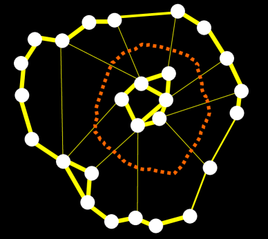
Figure 1.1: A weighted graph and its partition into two clusters.

A way to get around this problem is to normalize the cuts by dividing by some measure of each subset $A_{i}$. A solution using the volume $\mathrm{vol}(A_{i})$ of $A_{i}$ (for $K=2$) was proposed and investigated in a seminal paper of Shi and Malik [12]. Subsequently, Yu (in her dissertation [15]) and Yu and Shi [16] extended the method to $K>2$ clusters. The idea is to minimize the cost function

$$\mathrm{Ncut}(A_{1},\ldots,A_{K})=\sum_{i=1}^{K}\frac{\mathrm{links}(A_{i},\overline{A_{i}})}{\mathrm{vol}(A_{i})}=\sum_{i=1}^{K}\frac{\mathrm{cut}(A_{i},\overline{A_{i}})}{\mathrm{vol}(A_{i})}.$$

The first step is to express our optimization problem in matrix form. In the case of two clusters, a single vector $X$ can be used to describe the partition $(A_{1},A_{2})=(A,\overline{A})$. We need to choose the structure of this vector in such a way that

$$\mathrm{Ncut}(A,\overline{A})=\frac{X^{\top}LX}{X^{\top}DX},$$

where the term on the right-hand side is a Rayleigh ratio.

After careful study of the orginal papers, I discovered various facts that were implicit in these works, but I feel are important to be pointed out explicitly.

First, I realized that it is important to pick a vector representation which is invariant under multiplication by a nonzero scalar, because the Rayleigh ratio is scale-invariant, and it is crucial to take advantage of this fact to make the denominator go away. This implies that the solutions $X$ are points in the projective space $\mathbb{RP}^{N-1}$. This was my first revelation.

Let $N=|V|$ be the number of nodes in the graph $G$. In view of the desire for a scale-invariant representation, it is natural to assume that the vector $X$ is of the form

$$X=(x_{1},\ldots,x_{N}),$$

where $x_{i}\in\{a,b\}$ for $i=1,\ldots,N$, for any two distinct real numbers $a,b$. This is an indicator vector in the sense that, for $i=1,\ldots,N$,

$$x_{i}=\begin{cases}a&\text{if $v_{i}\in A$}\\ b&\text{if $v_{i}\notin A$}.\end{cases}$$

The choice $a=+1,b=-1$ is natural, but premature. The correct interpretation is really to view $X$ as a representative of a point in the real projective space $\mathbb{RP}^{N-1}$, namely the point $\mathbb{P}(X)$ of homogeneous coordinates $(x_{1}\colon\cdots\colon x_{N})$.

Let $d=\mathbf{1}^{\top}D\mathbf{1}$ and $\alpha=\mathrm{vol}(A)$. I prove that

$$\mathrm{Ncut}(A,\overline{A})=\frac{X^{\top}LX}{X^{\top}DX}$$

holds iff the following condition holds:

$$a\alpha+b(d-\alpha)=0. \dagger$$ ()

Note that condition $(\dagger)$ applied to a vector $X$ whose components are $a$ or $b$ is equivalent to the fact that $X$ is orthogonal to $D\mathbf{1}$, since

$$X^{\top}D\mathbf{1}=\alpha a+(d-\alpha)b,$$

where $\alpha=\mathrm{vol}(\{v_{i}\in V\mid x_{i}=a\})$.

If we let

$${\cal X}=\big{\{}(x_{1},\ldots,x_{N})\mid x_{i}\in\{a,b\},\>a,b\in\mathbb{R},\>a,b\not=0\big{\}},$$

our solution set is

$${\cal K}=\big{\{}X\in{\cal X}\mid X^{\top}D\mathbf{1}=0\big{\}}.$$

Actually, to be perfectly rigorous, we are looking for solutions in $\mathbb{RP}^{N-1}$, so our solution set is really

$$\mathbb{P}({\cal K})=\big{\{}(x_{1}\colon\cdots\colon x_{N})\in\mathbb{RP}^{N-1}\mid(x_{1},\ldots,x_{N})\in{\cal K}\big{\}}.$$

Consequently, our minimization problem can be stated as follows:

Problem PNC1

$$\mathrm{minimize} \frac{X^{\top}LX}{X^{\top}DX}$$

$$\mathrm{subject\ to} X^{\top}D\mathbf{1}=0, X\in{\cal X}.$$

It is understood that the solutions are points $\mathbb{P}(X)$ in $\mathbb{RP}^{N-1}$.

Since the Rayleigh ratio and the constraints $X^{\top}D\mathbf{1}=0$ and $X\in{\cal X}$ are scale-invariant, we are led to the following formulation of our problem:

Problem PNC2

$$\mathrm{minimize} X^{\top}LX$$

$$\mathrm{subject\ to} X^{\top}DX=1, X^{\top}D\mathbf{1}=0, X\in{\cal X}.$$

Problem PNC2 is equivalent to problem PNC1 in the sense that they have the same set of minimal solutions as points $\mathbb{P}(X)\in\mathbb{RP}^{N-1}$ given by their homogenous coordinates $X$. More precisely, if $X$ is any minimal solution of PNC1, then $X/(X^{\top}DX)^{1/2}$ is a minimal solution of PNC2 (with the same minimal value for the objective functions), and if $X$ is a minimal solution of PNC2, then $\lambda X$ is a minimal solution for PNC1 for all $\lambda\not=0$ (with the same minimal value for the objective functions).

Now, as in the classical papers, we consider the relaxation of the above problem obtained by dropping the condition that $X\in{\cal X}$, and proceed as usual. However, having found a solution $Z$ to the relaxed problem, we need to find a discrete solution $X$ such that $d(X,Z)$ is minimum in $\mathbb{RP}^{N-1}$. All this presented in Section 4.2.

If the number of clusters $K$ is at least $3$, then we need to choose a matrix representation for partitions on the set of vertices. It is important that such a representation be scale-invariant, and it is also necessary to state necessary and sufficient conditions for such matrices to represent a partition (to the best of our knowledge, these points are not clearly articulated in the literature).

We describe a partition $(A_{1},\ldots,A_{K})$ of the set of nodes $V$ by an $N\times K$ matrix $X=[X^{1}\cdots X^{K}]$ whose columns $X^{1},\ldots,X^{K}$ are indicator vectors of the partition $(A_{1},\ldots,A_{K})$. Inspired by what we did when $K=2$, we assume that the vector $X^{j}$ is of the form

$$X^{j}=(x_{1}^{j},\ldots,x_{N}^{j}),$$

where $x_{i}^{j}\in\{a_{j},b_{j}\}$ for $j=1,\ldots,K$ and $i=1,\ldots,N$, and where $a_{j},b_{j}$ are any two distinct real numbers. The vector $X^{j}$ is an indicator vector for $A_{j}$ in the sense that, for $i=1,\ldots,N$,

$$x_{i}^{j}=\begin{cases}a_{j}&\text{if $v_{i}\in A_{j}$}\\ b_{j}&\text{if $v_{i}\notin A_{j}$}.\end{cases}$$

The choice $\{a_{j},b_{j}\}=\{0,1\}$ for $j=1,\ldots,K$ is natural, but premature. I show that if we pick $b_{i}=0$, then we have

$$\frac{\mathrm{cut}(A_{j},\overline{A_{j}})}{\mathrm{vol}(A_{j})}=\frac{(X^{j})^{\top}LX^{j}}{(X^{j})^{\top}DX^{j}}\quad j=1,\ldots,K,$$

which implies that

$$\mathrm{Ncut}(A_{1},\ldots,A_{K})=\sum_{j=1}^{K}\frac{\mathrm{cut}(A_{j},\overline{A_{j}})}{\mathrm{vol}(A_{j})}=\sum_{j=1}^{K}\frac{(X^{j})^{\top}LX^{j}}{(X^{j})^{\top}DX^{j}}.$$

Then, I give necessary and sufficient conditions for a matrix $X$ to represent a partition.

If we let

$${\cal X}=\Big{\{}[X^{1}\>\ldots\>X^{K}]\mid X^{j}=a_{j}(x_{1}^{j},\ldots,x_{N}^{j}),\>x_{i}^{j}\in\{1,0\},a_{j}\in\mathbb{R},\>X^{j}\not=0\Big{\}}$$

(note that the condition $X^{j}\not=0$ implies that $a_{j}\not=0$), then the set of matrices representing partitions of $V$ into $K$ blocks is

$${\cal K}=\Big{\{}X=[X^{1}\>\cdots\>X^{K}]\quad\mid X\in{\cal X},$$

$$(X^{i})^{\top}DX^{j}=0,\quad 1\leq i,j\leq K,\>i\not=j,$$

$$X(X^{\top}X)^{-1}X^{\top}\mathbf{1}=\mathbf{1}\Big{\}}.$$

As in the case $K=2$, to be rigorous, the solution are really $K$-tuples of points in $\mathbb{RP}^{N-1}$, so our solution set is really

$$\mathbb{P}({\cal K})=\Big{\{}(\mathbb{P}(X^{1}),\ldots,\mathbb{P}(X^{K}))\mid[X^{1}\>\cdots\>X^{K}]\in{\cal K}\Big{\}}.$$

In view of the above, we have our first formulation of $K$-way clustering of a graph using normalized cuts, called problem PNC1 (the notation PNCX is used in Yu [15], Section 2.1):

$K$-way Clustering of a graph using Normalized Cut, Version 1:
Problem PNC1

$$\mathrm{minimize} \sum_{j=1}^{K}\frac{(X^{j})^{\top}LX^{j}}{(X^{j})^{\top}DX^{j}}$$

$$\mathrm{subject\ to} (X^{i})^{\top}DX^{j}=0,\quad 1\leq i,j\leq K,\>i\not=j,$$

$$X(X^{\top}X)^{-1}X^{\top}\mathbf{1}=\mathbf{1}, X\in{\cal X}.$$

As in the case $K=2$, the solutions that we are seeking are $K$-tuples $(\mathbb{P}(X^{1}),\ldots,\mathbb{P}(X^{K}))$ of points in $\mathbb{RP}^{N-1}$ determined by their homogeneous coordinates $X^{1},\ldots,X^{K}$.

Then, step by step, we transform problem PNC1 into an equivalent problem PNC2, which we eventually relax by dropping the condition that $X\in{\cal X}$.

Our second revelation is that the relaxation $(*_{1})$ of version 2 of our minimization problem (PNC2), which is equivalent to version 1, reveals that that the solutions of the relaxed problem $(*_{1})$ are members of the Grassmannian $G(K,N)$.

This leads us to our third revelation: we have two choices of metrics to compare solutions: (1) a metric on $(\mathbb{RP}^{N-1})^{K}$; (2) a metric on $G(K,N)$. We discuss the first choice, which is the choice implicitly adopted by Shi and Yu.

Some of the most technical material on the Rayleigh ratio, which is needed for some proofs in Chapter 3, is the object of Appendix A. Appendix B may seem a bit out of place. Its purpose is to explain how to define a metric on the projective space $\mathbb{RP}^{n}$. For this, we need to review a few notions of differential geometry.

I hope that these notes will be make it easier for people to become familiar with the wonderful theory of normalized graph cuts. As far as I know, except for a short section in one of Gilbert Strang’s book, and von Luxburg [14] excellent survey on spectral clustering, there is no comprehensive writing on the topic of normalized cuts.

Chapter 2 Graphs and Graph Laplacians; Basic Facts

2.1 Directed Graphs, Undirected Graphs, Incidence Matrices, Adjacency Matrices, Weighted Graphs

Definition 2.1.

A directed graph is a pair $G=(V,E)$, where $V=\{v_{1},\ldots,v_{m}\}$ is a set of nodes or vertices, and $E\subseteq V\times V$ is a set of ordered pairs of distinct nodes (that is, pairs $(u,v)\in V\times V$ with $u\not=v$), called edges. Given any edge $e=(u,v)$, we let $s(e)=u$ be the source of $e$ and $t(e)=v$ be the target of $e$.

Remark: Since an edge is a pair $(u,v)$ with $u\not=v$, self-loops are not allowed. Also, there is at most one edge from a node $u$ to a node $v$. Such graphs are sometimes called simple graphs.

An example of a directed graph is shown in Figure 2.1.

Figure 2.1: Graph $G_{1}$.

For every node $v\in V$, the degree $d(v)$ of $v$ is the number of edges leaving or entering $v$:

$$d(v)=|\{u\in V\mid(v,u)\in E\>\mathrm{or}\>(u,v)\in E\}|.$$

The degree matrix $D(G)$, is the diagonal matrix

$$D(G)=\mathrm{diag}(d_{1},\ldots,d_{m}).$$

For example, for graph $G_{1}$, we have

$$D(G_{1})=\begin{pmatrix}2&0&0&0&0\\ 0&4&0&0&0\\ 0&0&3&0&0\\ 0&0&0&3&0\\ 0&0&0&0&2\end{pmatrix}.$$

Unless confusion arises, we write $D$ instead of $D(G)$.

Definition 2.2.

Given a directed graph $G=(V,E)$, with $V=\{v_{1},\ldots,v_{m}\}$, if $E=\{e_{1},\ldots,e_{n}\}$, then the incidence matrix $\widetilde{D}(G)$ of $G$ is the $m\times n$ matrix whose entries $\widetilde{d}_{i\,j}$ are given by

$$\widetilde{d}_{i\,j}=\begin{cases}+1&\text{if $e_{j}=(v_{i},v_{k})$ for some $k$}\\ -1&\text{if $e_{j}=(v_{k},v_{i})$ for some $k$}\\ 0&\text{otherwise}.\end{cases}$$

Here is the incidence matrix of the graph $G_{1}$:

$$\widetilde{D}=\begin{pmatrix}1&1&0&0&0&0&0\\ -1&0&-1&-1&1&0&0\\ 0&-1&1&0&0&0&1\\ 0&0&0&1&0&-1&-1\\ 0&0&0&0&-1&1&0\end{pmatrix}.$$

Again, unless confusion arises, we write $\widetilde{D}$ instead of $\widetilde{D}(G)$.

Undirected graphs are obtained from directed graphs by forgetting the orientation of the edges.

Definition 2.3.

A graph (or undirected graph) is a pair $G=(V,E)$, where $V=\{v_{1},\ldots,v_{m}\}$ is a set of nodes or vertices, and $E$ is a set of two-element subsets of $V$ (that is, subsets $\{u,v\}$, with $u,v\in V$ and $u\not=v$), called edges.

Remark: Since an edge is a set $\{u,v\}$, we have $u\not=v$, so self-loops are not allowed. Also, for every set of nodes $\{u,v\}$, there there is at most one edge between $u$ and $v$. As in the case of directed graphs, such graphs are sometimes called simple graphs.

An example of a graph is shown in Figure 2.2.

Figure 2.2: The undirected graph $G_{2}$.

For every node $v\in V$, the degree $d(v)$ of $v$ is the number of edges adjacent to $v$:

$$d(v)=|\{u\in V\mid\{u,v\}\in E\}|.$$

The degree matrix $D$ is defined as before. The notion of incidence matrix for an undirected graph is not as useful as the in the case of directed graphs

Definition 2.4.

Given a graph $G=(V,E)$, with $V=\{v_{1},\ldots,v_{m}\}$, if $E=\{e_{1},\ldots,e_{n}\}$, then the incidence matrix $\widetilde{D}(G)$ of $G$ is the $m\times n$ matrix whose entries $\widetilde{d}_{i\,j}$ are given by

$$\widetilde{d}_{i\,j}=\begin{cases}+1&\text{if $e_{j}=\{v_{i},v_{k}\}$ for some $k$}\\ 0&\text{otherwise}.\end{cases}$$

Unlike the case of directed graphs, the entries in the incidence matrix of a graph (undirected) are nonnegative. We usally write $\widetilde{D}$ instead of $\widetilde{D}(G)$.

The notion of adjacency matrix is basically the same for directed or undirected graphs.

Definition 2.5.

Given a directed or undirected graph $G=(V,E)$, with $V=\{v_{1},\ldots,v_{m}\}$, the adjacency matrix $A(G)$ of $G$ is the symmetric $m\times m$ matrix $(a_{i\,j})$ such that

1. If $G$ is directed, then

   $$a_{i\,j}=\begin{cases}1&\text{if there is some edge $(v_{i},v_{j})\in E$ or some edge $(v_{j},v_{i})\in E$}\\ 0&\text{otherwise}.\end{cases}$$

2. Else if $G$ is undirected, then

   $$a_{i\,j}=\begin{cases}1&\text{if there is some edge $\{v_{i},v_{j}\}\in E$}\\ 0&\text{otherwise}.\end{cases}$$

As usual, unless confusion arises, we write $A$ instead of $A(G)$. Here is the adjacency matrix of both graphs $G_{1}$ and $G_{2}$:

$$A=\begin{pmatrix}0&1&1&0&0\\ 1&0&1&1&1\\ 1&1&0&1&0\\ 0&1&1&0&1\\ 0&1&0&1&0\end{pmatrix}.$$

In many applications, the notion of graph needs to be generalized to capture the intuitive idea that two nodes $u$ and $v$ are linked with a degree of certainty (or strength). Thus, we assign a nonnegative weights $w_{i\,j}$ to an edge $\{v_{i},v_{j}\}$; the smaller $w_{i\,j}$ is, the weaker is the link (or similarity) between $v_{i}$ and $v_{j}$, and the greater $w_{i\,j}$ is, the stronger is the link (or similarity) between $v_{i}$ and $v_{j}$.

Definition 2.6.

A weighted graph is a pair $G=(V,W)$, where $V=\{v_{1},\ldots,v_{m}\}$ is a set of nodes or vertices, and $W$ is a symmetric matrix called the weight matrix, such that $w_{i\,j}\geq 0$ for all $i,j\in\{1,\ldots,m\}$, and $w_{i\,i}=0$ for $i=1,\ldots,m$. We say that a set $\{v_{i},v_{j}\}$ is an edge iff $w_{i\,j}>0$. The corresponding (undirected) graph $(V,E)$ with $E=\{\{e_{i},e_{j}\}\mid w_{i\,j}>0\}$, is called the underlying graph of $G$.

Remark: Since $w_{i\,i}=0$, these graphs have no self-loops. We can think of the matrix $W$ as a generalized adjacency matrix. The case where $w_{i\,j}\in\{0,1\}$ is equivalent to the notion of a graph as in Definition 2.3.

We can think of the weight $w_{i\,j}$ of an edge $\{v_{i},v_{j}\}$ as a degree of similarity (or affinity) in an image, or a cost in a network. An example of a weighted graph is shown in Figure 2.3. The thickness of the edges corresponds to the magnitude of its weight.

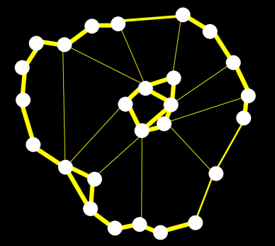
Figure 2.3: A weighted graph.

For every node $v_{i}\in V$, the degree $d(v_{i})$ of $v_{i}$ is the sum of the weights of the edges adjacent to $v_{i}$:

$$d(v_{i})=\sum_{j=1}^{m}w_{i\,j}.$$

Note that in the above sum, only nodes $v_{j}$ such that there is an edge $\{v_{i},v_{j}\}$ have a nonzero contribution. Such nodes are said to be adjacent to $v_{i}$. The degree matrix $D$ is defined as before, namely by $D=\mathrm{diag}(d(v_{1}),\ldots,d(v_{m}))$.

Following common practice, we denote by $\mathbf{1}$ the (column) vector whose components are all equal to $1$. Then, observe that $W\mathbf{1}$ is the (column) vector $(d(v_{1}),\ldots,d(v_{m}))$ consisting of the degrees of the nodes of the graph.

Given any subset of nodes $A\subseteq V$, we define the volume $\mathrm{vol}(A)$ of $A$ as the sum of the weights of all edges adjacent to nodes in $A$:

$$\mathrm{vol}(A)=\sum_{v_{i}\in A}d(v_{i})=\sum_{v_{i}\in A}\sum_{j=1}^{m}w_{i\,j}.$$

Remark: Yu and Shi [16] use the notation $\mathrm{degree}(A)$ instead of $\mathrm{vol}(A)$.

The notions of degree and volume are illustrated in Figure 2.4.

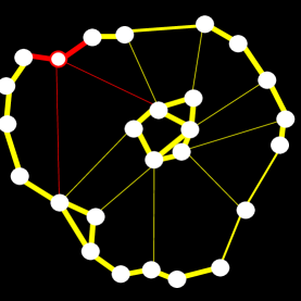
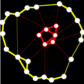
Figure 2.4: Degree and volume.

Observe that $\mathrm{vol}(A)=0$ if $A$ consists of isolated vertices, that is, if $w_{i\,j}=0$ for all $v_{i}\in A$. Thus, it is best to assume that $G$ does not have isolated vertices.

Given any two subset $A,B\subseteq V$ (not necessarily distinct), we define $\mathrm{links}(A,B)$ by

$$\mathrm{links}(A,B)=\sum_{v_{i}\in A,v_{j}\in B}w_{i\,j}.$$

Since the matrix $W$ is symmetric, we have

$$\mathrm{links}(A,B)=\mathrm{links}(B,A),$$

and observe that $\mathrm{vol}(A)=\mathrm{links}(A,V)$.

The quantity $\mathrm{links}(A,\overline{A})=\mathrm{links}(\overline{A},A)$, where $\overline{A}=V-A$ denotes the complement of $A$ in $V$, measures how many links escape from $A$ (and $\overline{A}$), and the quantity $\mathrm{links}(A,A)$ measures how many links stay within $A$ itself. The quantity

$$\mathrm{cut}(A)=\mathrm{links}(A,\overline{A})$$

is often called the cut of $A$, and the quantity

$$\mathrm{assoc}(A)=\mathrm{links}(A,A)$$

is often called the association of $A$. Clearly,

$$\mathrm{cut}(A)+\mathrm{assoc}(A)=\mathrm{vol}(A).$$

The notions of cut is illustrated in Figure 2.5.

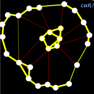
Figure 2.5: A Cut involving the set of nodes in the center and the nodes on the perimeter.

We now define the most important concept of these notes: The Laplacian matrix of a graph. Actually, as we will see, it comes in several flavors.

2.2 Laplacian Matrices of Graphs

Let us begin with directed graphs, although as we will see, graph Laplacians are fundamentally associated with undirected graph. The key proposition whose proof can be found in Gallier [5] and Godsil and Royle [8] is this:

Proposition 2.1.

Given any directed graph $G$ if $\widetilde{D}$ is the incidence matrix of $G$, $A$ is the adjacency matrix of $G$, and $D$ is the degree matrix such that $D_{i\,i}=d(v_{i})$, then

$$\widetilde{D}\widetilde{D}^{\top}=D-A.$$

Consequently, $\widetilde{D}\widetilde{D}^{\top}$ is independent of the orientation of $G$ and $D-A$ is symmetric, positive, semidefinite; that is, the eigenvalues of $D-A$ are real and nonnegative.

The matrix $L=\widetilde{D}\widetilde{D}^{\top}=D-A$ is called the (unnormalized) graph Laplacian of the graph $G$. For example, the graph Laplacian of graph $G_{1}$ is

$$L=\begin{pmatrix}2&-1&-1&0&0\\ -1&4&-1&-1&-1\\ -1&-1&3&-1&0\\ 0&-1&-1&3&-1\\ 0&-1&0&-1&2\end{pmatrix}.$$

The (unnormalized) graph Laplacian of an undirected graph $G=(V,E)$ is defined by

$$L=D-A.$$

Since $L$ is equal to $\widetilde{D}\widetilde{D}^{\top}$ for any orientation of $G$, it is also positive semidefinite. Observe that each row of $L$ sums to zero. Consequently, the vector $\mathbf{1}$ is in the nullspace of $L$.

Remark: With the unoriented version of the incidence matrix (see Definition 2.4), it can be shown that

$$\widetilde{D}\widetilde{D}^{\top}=D+A.$$

The natural generalization of the notion of graph Laplacian to weighted graphs is this:

Definition 2.7.

Given any weighted directed graph $G=(V,W)$ with $V=\{v_{1},\ldots,v_{m}\}$, the (unnormalized) graph Laplacian $L(G)$ of $G$ is defined by

$$L(G)=D(G)-W,$$

where $D(G)=\mathrm{diag}(d_{1},\ldots,d_{m})$ is the degree matrix of $G$ (a diagonal matrix), with

$$d_{i}=\sum_{j=1}^{m}w_{i\,j}.$$

As usual, unless confusion arises, we write $L$ instead of $L(G)$.

It is clear that each row of $L$ sums to $0$, so the vector $\mathbf{1}$ is the nullspace of $L$, but it is less obvious that $L$ is positive semidefinite. An easy way to prove this is to evaluate the quadratic form $x^{\top}Lx$.

Proposition 2.2.

For any $m\times m$ symmetric matrix $W$, if we let $L=D-W$ where $D$ is the degree matrix of $W=(w_{ij})$, then we have

$$x^{\top}Lx=\frac{1}{2}\sum_{i,j=1}^{m}w_{i\,j}(x_{i}-x_{j})^{2}\quad\mathrm{for\ all}\>x\in\mathbb{R}^{m}.$$

Consequently, $x^{\top}Lx$ does not depend on the diagonal entries in $W$, and if $w_{i\,j}\geq 0$ for all $i,j\in\{1,\ldots,m\}$, then $L$ is positive semidefinite.

Proof.

We have

$$x^{\top}Lx =x^{\top}Dx-x^{\top}Wx$$

$$=\sum_{i=1}^{m}d_{i}x_{i}^{2}-\sum_{i,j=1}^{m}w_{i\,j}x_{i}x_{j}$$

$$=\frac{1}{2}\left(\sum_{i=1}^{m}d_{i}x_{i}^{2}-2\sum_{i,j=1}^{m}w_{i\,j}x_{i}x_{j}+\sum_{i=1}^{m}d_{i}x_{i}^{2}\right)$$

$$=\frac{1}{2}\sum_{i,j=1}^{m}w_{i\,j}(x_{i}-x_{j})^{2}.$$

Obviously, the quantity on the right-hand side does not depend on the diagonal entries in $W$, and if if $w_{i\,j}\geq 0$ for all $i,j$, then this quantity is nonnegative. ∎

Proposition 2.2 immediately implies the following facts: For any weighted graph $G=(V,W)$,

1. The eigenvalues $0=\lambda_{1}\leq\lambda_{2}\leq\ldots\leq\lambda_{m}$ of $L$ are real and nonnegative, and there is an orthonormal basis of eigenvectors of $L$.

2. The smallest eigenvalue $\lambda_{1}$ of $L$ is equal to $0$, and $\mathbf{1}$ is a corresponding eigenvector.

It turns out that the dimension of the nullspace of $L$ (the eigenspace of $0$) is equal to the number of connected components of the underlying graph of $G$.

Proposition 2.3.

Let $G=(V,W)$ be a ,weighted graph. The number $c$ of connected components $K_{1},\ldots,K_{c}$ of the underlying graph of $G$ is equal to the dimension of the nullspace of $L$, which is equal to the multiplicity of the eigenvalue $0$. Furthermore, the nullspace of $L$ has a basis consisting of indicator vectors of the connected components of $G$, that is, vectors $(f_{1},\ldots,f_{m})$ such that $f_{j}=1$ iff $v_{j}\in K_{i}$ and $f_{j}=0$ otherwise.

Proof.

A complete proof can be found in von Luxburg [14], and we only give a sketch of the proof.

First, assume that $G$ is connected, so $c=1$. A nonzero vector $x$ is in the kernel of $L$ iff $Lx=0$, which implies that

$$x^{\top}Lx=\frac{1}{2}\sum_{i,j=1}^{m}w_{i\,j}(x_{i}-x_{j})^{2}=0.$$

This implies that $x_{i}=x_{j}$ whenever $w_{i\,j}>0$, and thus, $x_{i}=x_{j}$ whenever nodes $v_{i}$ and $v_{j}$ are linked by an edge. By induction, $x_{i}=x_{j}$ whenever there is a path from $v_{i}$ to $v_{j}$. Since $G$ is assumed to be connected, any two nodes are linked by a path, which implies that $x_{i}=x_{j}$ for all $i\not=j$. Therefore, the nullspace of $L$ is spanned by $\mathbf{1}$, which is indeed the indicator vector of $K_{1}=V$, and this nullspace has dimension $1$.

Let us now assume that $G$ has $c\geq 2$ connected components. If so, by renumbering the rows and columns of $W$, we may assume that $W$ is a block matrix consisting of $c$ blocks, and similarly $L$ is a block matrix of the form

$$L=\begin{pmatrix}L_{1}&&&\\ &L_{2}&&\\ &&\ddots&\\ &&&L_{c}\end{pmatrix},$$

where $L_{i}$ is the graph Laplacian associated with the connected component $K_{i}$. By the induction hypothesis, $0$ is an eigenvalue of multiplicity $1$ for each $L_{i}$, and so the nullspace of $L$ has dimension $c$. The rest is left as an exercise (or see von Luxburg [14]). ∎

Proposition 2.3 implies that if the underlying graph of $G$ is connected, then the second eigenvalue, $\lambda_{2}$, of $L$ is strictly positive.

Remarkably, the eigenvalue $\lambda_{2}$ contains a lot of information about the graph $G$ (assuming that $G=(V,E)$ is an undirected graph). This was first discovered by Fiedler in 1973, and for this reason, $\lambda_{2}$ is often referred to as the Fiedler number. For more on the properties of the Fiedler number, see Godsil and Royle [8] (Chapter 13) and Chung [3]. More generally, the spectrum $(0,\lambda_{2},\ldots,\lambda_{m})$ of $L$ contains a lot of information about the combinatorial structure of the graph $G$. Leverage of this information is the object of spectral graph theory.

It turns out that normalized variants of the graph Laplacian are needed, especially in applications to graph clustering. These variants make sense only if $G$ has no isolated vertices, which means that every row of $W$ contains some strictly positive entry. In this case, the degree matrix $D$ contains positive entries, so it is invertible and $D^{-1/2}$ makes sense; namely

$$D^{-1/2}=\mathrm{diag}(d_{1}^{-1/2},\ldots,d_{m}^{-1/2}),$$

and similarly for any real exponent $\alpha$.

Definition 2.8.

Given any weighted directed graph $G=(V,W)$ with no isolated vertex and with $V=\{v_{1},\ldots,v_{m}\}$, the (normalized) graph Laplacians $L_{\mathrm{sym}}$ and $L_{\mathrm{rw}}$ of $G$ are defined by

$$L_{\mathrm{sym}} =D^{-1/2}LD^{-1/2}=I-D^{-1/2}WD^{-1/2}$$

$$L_{\mathrm{rw}} =D^{-1}L=I-D^{-1}W.$$

Observe that the Laplacian $L_{\mathrm{sym}}=D^{-1/2}LD^{-1/2}$ is a symmetric matrix (because $L$ and $D^{-1/2}$ are symmetric) and that

$$L_{\mathrm{rw}}=D^{-1/2}L_{\mathrm{sym}}D^{1/2}.$$

The reason for the notation $L_{\mathrm{rw}}$ is that this matrix is closely related to a random walk on the graph $G$. There are simple relationships between the eigenvalues and the eigenvectors of $L_{\mathrm{sym}}$, and $L_{\mathrm{rw}}$. There is also a simple relationship with the generalized eigenvalue problem $Lx=\lambda Dx$.

Proposition 2.4.

Let $G=(V,W)$ be a weighted graph without isolated vertices. The graph Laplacians, $L,L_{\mathrm{sym}}$, and $L_{\mathrm{rw}}$ satisfy the following properties:

1. The matrix $L_{\mathrm{sym}}$ is symmetric, positive, semidefinite. In fact,

   $$x^{\top}L_{\mathrm{sym}}x=\frac{1}{2}\sum_{i,j=1}^{m}w_{i\,j}\left(\frac{x_{i}}{\sqrt{d_{i}}}-\frac{x_{j}}{\sqrt{d_{j}}}\right)^{2}\quad\mathrm{for\ all}\>x\in\mathbb{R}^{m}.$$

2. The normalized graph Laplacians $L_{\mathrm{sym}}$ and $L_{\mathrm{rw}}$ have the same spectrum
   $(0=\nu_{1}\leq\nu_{2}\leq\ldots\leq\nu_{m})$, and a vector $u\not=0$ is an eigenvector of $L_{\mathrm{rw}}$ for $\lambda$ iff $D^{1/2}u$ is an eigenvector of $L_{\mathrm{sym}}$ for $\lambda$.

3. The graph Laplacians, $L,L_{\mathrm{sym}}$, and $L_{\mathrm{rw}}$ are symmetric, positive, semidefinite.

4. A vector $u\not=0$ is a solution of the generalized eigenvalue problem $Lu=\lambda Du$ iff $D^{1/2}u$ is an eigenvector of $L_{\mathrm{sym}}$ for the eigenvalue $\lambda$ iff $u$ is an eigenvector of $L_{\mathrm{rw}}$ for the eigenvalue $\lambda$.

5. The graph Laplacians, $L$ and $L_{\mathrm{rw}}$ have the same nullspace.

6. The vector $\mathbf{1}$ is in the nullspace of $L_{\mathrm{rw}}$, and $D^{1/2}\mathbf{1}$ is in the nullspace of $L_{\mathrm{sym}}$.

Proof.

(1) We have $L_{\mathrm{sym}}=D^{-1/2}LD^{-1/2}$, and $D^{-1/2}$ is a symmetric invertible matrix (since it is an invertible diagonal matrix). It is a well-known fact of linear algebra that if $B$ is an invertible matrix, then a matrix $S$ is symmetric, positive semidefinite iff $BSB^{\top}$ is symmetric, positive semidefinite. Since $L$ is symmetric, positive semidefinite, so is $L_{\mathrm{sym}}=D^{-1/2}LD^{-1/2}$. The formula

$$x^{\top}L_{\mathrm{sym}}x=\frac{1}{2}\sum_{i,j=1}^{m}w_{i\,j}\left(\frac{x_{i}}{\sqrt{d_{i}}}-\frac{x_{j}}{\sqrt{d_{j}}}\right)^{2}\quad\mathrm{for\ all}\>x\in\mathbb{R}^{m}$$

follows immediately from Proposition 2.2 by replacing $x$ by $D^{-1/2}x$, and also shows that $L_{\mathrm{sym}}$ is positive semidefinite.

(2) Since

$$L_{\mathrm{rw}}=D^{-1/2}L_{\mathrm{sym}}D^{1/2},$$

the matrices $L_{\mathrm{sym}}$ and $L_{\mathrm{rw}}$ are similar, which implies that they have the same spectrum. In fact, since $D^{1/2}$ is invertible,

$$L_{\mathrm{rw}}u=D^{-1}Lu=\lambda u$$

iff

$$D^{-1/2}Lu=\lambda D^{1/2}u$$

iff

$$D^{-1/2}LD^{-1/2}D^{1/2}u=L_{\mathrm{sym}}D^{1/2}u=\lambda D^{1/2}u,$$

which shows that a vector $u\not=0$ is an eigenvector of $L_{\mathrm{rw}}$ for $\lambda$ iff $D^{1/2}u$ is an eigenvector of $L_{\mathrm{sym}}$ for $\lambda$.

(3) We already know that $L$ and $L_{\mathrm{sym}}$ are positive semidefinite, and (2) shows that $L_{\mathrm{rw}}$ is also positive semidefinite.

(4) Since $D^{-1/2}$ is invertible, we have

$$Lu=\lambda Du$$

iff

$$D^{-1/2}Lu=\lambda D^{1/2}u$$

iff

$$D^{-1/2}LD^{-1/2}D^{1/2}u=L_{\mathrm{sym}}D^{1/2}u=\lambda D^{1/2}u,$$

which shows that a vector $u\not=0$ is a solution of the generalized eigenvalue problem $Lu=\lambda Du$ iff $D^{1/2}u$ is an eigenvector of $L_{\mathrm{sym}}$ for the eigenvalue $\lambda$. The second part of the statement follows from (2).

(5) Since $D^{-1}$ is invertible, we have $Lu=0$ iff $D^{-1}u=L_{\mathrm{rw}}u=0$.

(6) Since $L\mathbf{1}=0$, we get $L_{\mathrm{rw}}u=D^{-1}L\mathbf{1}=0$. That $D^{1/2}\mathbf{1}$ is in the nullspace of $L_{\mathrm{sym}}$ follows from (2). ∎

A version of Proposition 2.5 also holds for the graph Laplacians $L_{\mathrm{sym}}$ and $L_{\mathrm{rw}}$. The proof is left as an exercise.

Proposition 2.5.

Let $G=(V,W)$ be a weighted graph. The number $c$ of connected components $K_{1},\ldots,K_{c}$ of the underlying graph of $G$ is equal to the dimension of the nullspace of both $L_{\mathrm{sym}}$ and $L_{\mathrm{rw}}$, which is equal to the multiplicity of the eigenvalue $0$. Furthermore, the nullspace of $L_{\mathrm{rw}}$ has a basis consisting of indicator vectors of the connected components of $G$, that is, vectors $(f_{1},\ldots,f_{m})$ such that $f_{j}=1$ iff $v_{j}\in K_{i}$ and $f_{j}=0$ otherwise. For $L_{\mathrm{sym}}$, a basis of the nullpace is obtained by multipying the above basis of the nullspace of $L_{\mathrm{rw}}$ by $D^{1/2}$.

Chapter 3 Spectral Graph Drawing

3.1 Graph Drawing and Energy Minimization

Let $G=(V,E)$ be some undirected graph. It is often desirable to draw a graph, usually in the plane but possibly in 3D, and it turns out that the graph Laplacian can be used to design surprisingly good methods. Say $|V|=m$. The idea is to assign a point $\rho(v_{i})$ in $\mathbb{R}^{n}$ to the vertex $v_{i}\in V$, for every $v_{i}\in V$, and to draw a line segment between the points $\rho(v_{i})$ and $\rho(v_{j})$. Thus, a graph drawing is a function $\rho\colon V\rightarrow\mathbb{R}^{n}$.

We define the matrix of a graph drawing $\rho$ (in $\mathbb{R}^{n}$) as a $m\times n$ matrix $R$ whose $i$th row consists of the row vector $\rho(v_{i})$ corresponding to the point representing $v_{i}$ in $\mathbb{R}^{n}$. Typically, we want $n<m$; in fact $n$ should be much smaller than $m$. A representation is balanced iff the sum of the entries of every column is zero, that is,

$$\mathbf{1}^{\top}R=0.$$

If a representation is not balanced, it can be made balanced by a suitable translation. We may also assume that the columns of $R$ are linearly independent, since any basis of the column space also determines the drawing. Thus, from now on, we may assume that $n\leq m$.

Remark: A graph drawing $\rho\colon V\rightarrow\mathbb{R}^{n}$ is not required to be injective, which may result in degenerate drawings where distinct vertices are drawn as the same point. For this reason, we prefer not to use the terminology graph embedding, which is often used in the literature. This is because in differential geometry, an embedding always refers to an injective map. The term graph immersion would be more appropriate.

As explained in Godsil and Royle [8], we can imagine building a physical model of $G$ by connecting adjacent vertices (in $\mathbb{R}^{n}$) by identical springs. Then, it is natural to consider a representation to be better if it requires the springs to be less extended. We can formalize this by defining the energy of a drawing $R$ by

$${\cal E}(R)=\sum_{\{v_{i},v_{j}\}\in E}\left\|\rho(v_{i})-\rho(v_{j})\right\|^{2},$$

where $\rho(v_{i})$ is the $i$th row of $R$ and $\left\|\rho(v_{i})-\rho(v_{j})\right\|^{2}$ is the square of the Euclidean length of the line segment joining $\rho(v_{i})$ and $\rho(v_{j})$.

Then, “good drawings” are drawings that minimize the energy function ${\cal E}$. Of course, the trivial representation corresponding to the zero matrix is optimum, so we need to impose extra constraints to rule out the trivial solution.

We can consider the more general situation where the springs are not necessarily identical. This can be modeled by a symmetric weight (or stiffness) matrix $W=(w_{ij})$, with $w_{ij}\geq 0$. Then our energy function becomes

$${\cal E}(R)=\sum_{\{v_{i},v_{j}\}\in E}w_{ij}\left\|\rho(v_{i})-\rho(v_{j})\right\|^{2}.$$

It turns out that this function can be expressed in terms of the matrix $R$ and a diagonal matrix $\widehat{W}$ obtained from $W$. Let $p=|E|$ be the number of edges in $E$ and pick any enumeration of these edges, so that every edge $\{v_{i},v_{j}\}$ is uniquely represented by some index $e$. Then, let $\widehat{W}$ be the $p\times p$ diagonal matrix such that

$$\widehat{w}_{ee}=w_{ij},\quad\text{where $e$ correspond to the edge $\{v_{i},v_{j}\}$}.$$

We have the following proposition from Godsil and Royle [8].

Proposition 3.1.

Let $G=(V,E)$ be an undirected graph, with $|V|=m$, $|E|=p$, let $W$ be a $m\times m$ weight matrix, and let $R$ be the matrix of a graph drawing $\rho$ of $G$ in $\mathbb{R}^{n}$ (a $m\times n$ matrix). If $\widetilde{D}$ is the incidence matrix associated with any orientation of the graph $G$, and $\widehat{W}$ is the $p\times p$ diagonal matrix associated with $W$, then

$${\cal E}(R)=\mathrm{tr}(R^{\top}\widetilde{D}\widehat{W}\widetilde{D}^{\top}R).$$

Proof.

Observe that the rows of $\widetilde{D}^{\top}R$ are indexed by the edges of $G$, and if $\{v_{i},v_{j}\}\in E$, then the $e$th row of $\widetilde{D}^{\top}R$ is

$$\pm(\rho(v_{i})-\rho(v_{j})),$$

where $e$ is the index corresponding to the edge $\{v_{i},v_{j}\}$. As a consequence, the diagonal entries of $\widetilde{D}^{\top}RR^{\top}\widetilde{D}$ have the form $\left\|\rho(v_{i})-\rho(v_{j})\right\|^{2}$, where $\{v_{i},v_{j}\}$ ranges over the edges in $E$. Hence,

$${\cal E}(R)=\mathrm{tr}(\widehat{W}\widetilde{D}^{\top}RR^{\top}\widetilde{D})=\mathrm{tr}(R^{\top}\widetilde{D}\widehat{W}\widetilde{D}^{\top}R),$$

since $\mathrm{tr}(AB)=\mathrm{tr}(BA)$ for any two matrices $A$ and $B$. ∎

The matrix

$$L=\widetilde{D}\widehat{W}\widetilde{D}^{\top}$$

may be viewed as a weighted Laplacian of $G$. Observe that $L$ is a $m\times m$ matrix, and that

$$L_{ij}=\begin{cases}-w_{ij}&\text{if $i\not=j$}\\ \sum_{\{v_{i},v_{k}\}\in E}w_{ik}&\text{if $i=j$}.\end{cases}$$

Therefore,

$$L=D-W,$$

the familiar unnormalized Laplacian matrix associated with $W$, where $D$ is the degree matrix associated with $W$, and so

$${\cal E}(R)=\mathrm{tr}(R^{\top}LR).$$

Note that

$$L\mathbf{1}=0,$$

as we already observed.

Since the matrix $R^{\top}\widetilde{D}\widehat{W}\widetilde{D}^{\top}R=R^{\top}LR$ is symmetric, it has real eigenvalues. Actually, since $L=\widetilde{D}\widehat{W}\widetilde{D}^{\top}$ is positive semidefinite, so is $R^{\top}LR$. Then, the trace of $R^{\top}LR$ is equal to the sum of its positive eigenvalues, and this is the energy ${\cal E}(R)$ of the graph drawing.

If $R$ is the matrix of a graph drawing in $\mathbb{R}^{n}$, then for any invertible matrix $M$, the map that assigns $v_{i}$ to $\rho(v_{i})M$ is another graph drawing of $G$, and these two drawings convey the same amount of information. From this point of view, a graph drawing is determined by the column space of $R$. Therefore, it is reasonable to assume that the columns of $R$ are pairwise orthogonal and that they have unit length. Such a matrix satisfies the equation $R^{\top}R=I$, and the corresponding drawing is called an orthogonal drawing. This condition also rules out trivial drawings. The following result tells us how to find minimum energy graph drawings, provided the graph is connected.

Theorem 3.2.

Let $G=(V,W)$ be a weigted graph with $|V|=m$. If $L=D-W$ is the (unnormalized) Laplacian of $G$, and if the eigenvalues of $L$ are $0=\lambda_{1}<\lambda_{2}\leq\lambda_{3}\leq\ldots\leq\lambda_{m}$, then the minimal energy of any balanced orthogonal graph drawing of $G$ in $\mathbb{R}^{n}$ is equal to $\lambda_{2}+\cdots+\lambda_{n+1}$ (in particular, this implies that $n<m$). The $m\times n$ matrix $R$ consisting of any unit eigenvectors $u_{2},\ldots,u_{n+1}$ associated with $\lambda_{2}\leq\ldots\leq\lambda_{n+1}$ yields an orthogonal graph drawing of minimal energy; it satisfies the condition $R^{\top}R=I$.

Proof.

We present the proof given in Godsil and Royle [8] (Section 13.4, Theorem 13.4.1). The key point is that the sum of the $n$ smallest eigenvalues of $L$ is a lower bound for $\mathrm{tr}(R^{\top}LR)$. This can be shown using an argument using the Rayleigh ratio; see Proposition A.3. Then, any $n$ eigenvectors $(u_{1},\ldots,u_{n})$ associated with $\lambda_{1},\ldots,\lambda_{n}$ achieve this bound. Because the first eigenvalue of $L$ is $\lambda_{1}=0$ and because we are assuming that $\lambda_{2}>0$, we have $u_{1}=\mathbf{1}/\sqrt{m}$, and by deleting $u_{1}$ we obtain a balanced orthogonal graph drawing in $\mathbb{R}^{n-1}$ with the same energy. The converse is true, so the minimum energy of an orthogonal graph drawing in $\mathbb{R}^{n}$ is equal to the minimum energy of an orthogonal graph drawing in $\mathbb{R}^{n+1}$, and this minimum is $\lambda_{2}+\cdots+\lambda_{n+1}$. The rest is clear. ∎

Observe that for any orthogonal $n\times n$ matrix $Q$, since

$$\mathrm{tr}(R^{\top}LR)=\mathrm{tr}(Q^{\top}R^{\top}LRQ),$$

the matrix $RQ$ also yields a minimum orthogonal graph drawing.

In summary, if $\lambda_{2}>0$, an automatic method for drawing a graph in $\mathbb{R}^{2}$ is this:

1. Compute the two smallest nonzero eigenvalues $\lambda_{2}\leq\lambda_{3}$ of the graph Laplacian $L$ (it is possible that $\lambda_{3}=\lambda_{2}$ if $\lambda_{2}$ is a multiple eigenvalue);

2. Compute two unit eigenvectors $u_{2},u_{3}$ associated with $\lambda_{2}$ and $\lambda_{3}$, and let $R=[u_{2}\>u_{3}]$ be the $m\times 2$ matrix having $u_{2}$ and $u_{3}$ as columns.

3. Place vertex $v_{i}$ at the point whose coordinates is the $i$th row of $R$, that is, $(R_{i1},R_{i2})$.

This method generally gives pleasing results, but beware that there is no guarantee that distinct nodes are assigned distinct images, because $R$ can have identical rows. This does not seem to happen often in practice.

3.2 Examples of Graph Drawings

We now give a number of examples using Matlab. Some of these are borrowed or adapted from Spielman [13].

Example 1. Consider the graph with four nodes whose adjacency matrix is

$$A=\begin{pmatrix}0&1&1&0\\ 1&0&0&1\\ 1&0&0&1\\ 0&1&1&0\end{pmatrix}.$$

We use the following program to compute $u_{2}$ and $u_{3}$:

A = [0 1 1 0; 1 0 0 1; 1 0 0 1; 0 1 1 0];
D = diag(sum(A));
L = D - A;
[v, e] = eigs(L);
gplot(A, v(:,[3 2]))
hold on;
gplot(A, v(:,[3 2]),’o’)

The graph of Example 1 is shown in Figure 3.1. The function eigs(L) computes the six largest eigenvalues of $L$ in decreasing order, and corresponding eigenvectors. It turns out that $\lambda_{2}=\lambda_{3}=2$ is a double eigenvalue.

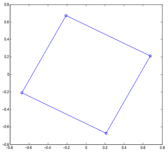
Figure 3.1: Drawing of the graph from Example 1.

Example 2. Consider the graph $G_{2}$ shown in Figure 2.2 given by the adjacency matrix

$$A=\begin{pmatrix}0&1&1&0&0\\ 1&0&1&1&1\\ 1&1&0&1&0\\ 0&1&1&0&1\\ 0&1&0&1&0\end{pmatrix}.$$

We use the following program to compute $u_{2}$ and $u_{3}$:

A = [0 1 1 0 0; 1 0 1 1 1; 1 1 0 1 0; 0 1 1 0 1; 0 1 0 1 0];
D = diag(sum(A));
L = D - A;
[v, e] = eig(L);
gplot(A, v(:, [2 3]))
hold on
gplot(A, v(:, [2 3]),’o’)

The function eig(L) (with no s at the end) computes the eigenvalues of $L$ in increasing order. The result of drawing the graph is shown in Figure 3.2. Note that node $v_{2}$ is assigned to the point $(0,0)$, so the difference between this drawing and the drawing in Figure 2.2 is that the drawing of Figure 3.2 is not convex.

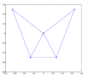
Figure 3.2: Drawing of the graph from Example 2.

Example 3. Consider the ring graph defined by the adjacency matrix $A$ given in the Matlab program shown below:

A = diag(ones(1, 11),1);
A = A + A’;
A(1, 12) = 1; A(12, 1) = 1;
D = diag(sum(A));
L = D - A;
[v, e] = eig(L);
gplot(A, v(:, [2 3]))
hold on
gplot(A, v(:, [2 3]),’o’)

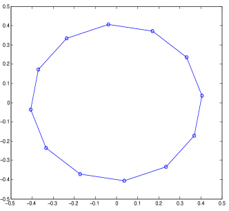
Figure 3.3: Drawing of the graph from Example 3.

Observe that we get a very nice ring; see Figure 3.3. Again $\lambda_{2}=0.2679$ is a double eigenvalue (and so are the next pairs of eigenvalues, except the last, $\lambda_{12}=4$).

Example 4. In this example adpated from Spielman, we generate $20$ randomly chosen points in the unit square, compute their Delaunay triangulation, then the adjacency matrix of the corresponding graph, and finally draw the graph using the second and third eigenvalues of the Laplacian.

A = zeros(20,20);
xy = rand(20, 2);
trigs = delaunay(xy(:,1), xy(:,2));
elemtrig = ones(3) - eye(3);
for i = 1:length(trigs),
 A(trigs(i,:),trigs(i,:)) = elemtrig;
end
A = double(A >0);
gplot(A,xy)
D = diag(sum(A));
L = D - A;
[v, e] = eigs(L, 3, ’sm’);
figure(2)
gplot(A, v(:, [2 1]))
hold on
gplot(A, v(:, [2 1]),’o’)

The Delaunay triangulation of the set of $20$ points and the drawing of the corresponding graph are shown in Figure 3.4. The graph drawing on the right looks nicer than the graph on the left but is is no longer planar.

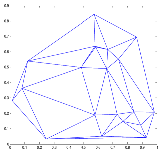
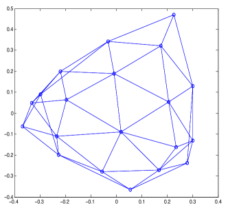
Figure 3.4: Delaunay triangulation (left) and drawing of the graph from Example 4 (right).

Example 5. Our last example, also borrowed from Spielman [13], corresponds to the skeleton of the “Buckyball,”, a geodesic dome invented by the architect Richard Buckminster Fuller (1895–1983). The Montréal Biosphère is an example of a geodesic dome designed by Buckminster Fuller.

A = full(bucky);
D = diag(sum(A));
L = D - A;
[v, e] = eig(L);
gplot(A, v(:, [2 3]))
hold on;
gplot(A,v(:, [2 3]), ’o’)

Figure 3.5 shows a graph drawing of the Buckyball. This picture seems a bit squashed for two reasons. First, it is really a $3$-dimensional graph; second, $\lambda_{2}=0.2434$ is a triple eigenvalue. (Actually, the Laplacian of $L$ has many multiple eigenvalues.) What we should really do is to plot this graph in $\mathbb{R}^{3}$ using three orthonormal eigenvectors associated with $\lambda_{2}$.

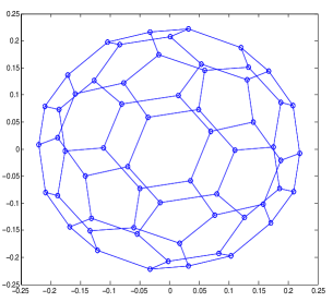
Figure 3.5: Drawing of the graph of the Buckyball.

A $3$D picture of the graph of the Buckyball is produced by the following Matlab program, and its image is shown in Figure 3.6. It looks better!

[x, y] = gplot(A, v(:, [2 3]));
[x, z] = gplot(A, v(:, [2 4]));
plot3(x,y,z)

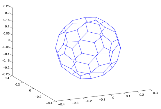
Figure 3.6: Drawing of the graph of the Buckyball in $\mathbb{R}^{3}$.

Chapter 4 Graph Clustering

4.1 Graph Clustering Using Normalized Cuts

Given a set of data, the goal of clustering is to partition the data into different groups according to their similarities. When the data is given in terms of a similarity graph $G$, where the weight $w_{i\,j}$ between two nodes $v_{i}$ and $v_{j}$ is a measure of similarity of $v_{i}$ and $v_{j}$, the problem can be stated as follows: Find a partition $(A_{1},\ldots,A_{K})$ of the set of nodes $V$ into different groups such that the edges between different groups have very low weight (which indicates that the points in different clusters are dissimilar), and the edges within a group have high weight (which indicates that points within the same cluster are similar).

The above graph clustering problem can be formalized as an optimization problem, using the notion of cut mentioned at the end of Section 2.1.

Given a subset $A$ of the set of vertices $V$, recall that we define $\mathrm{cut}(A)$ by

$$\mathrm{cut}(A)=\mathrm{links}(A,\overline{A})=\sum_{v_{i}\in A,v_{j}\in\overline{A}}w_{i\,j},$$

and that

$$\mathrm{cut}(A)=\mathrm{links}(A,\overline{A})=\mathrm{links}(\overline{A},A)=\mathrm{cut}(\overline{A}).$$

If we want to partition $V$ into $K$ clusters, we can do so by finding a partition ($A_{1},\ldots,A_{K}$) that minimizes the quantity

$$\mathrm{cut}(A_{1},\ldots,A_{K})=\frac{1}{2}\sum_{1=1}^{K}\mathrm{cut}(A_{i}).$$

The reason for introducing the factor $1/2$ is to avoiding counting each edge twice. In particular,

$$\mathrm{cut}(A,\overline{A})=\mathrm{links}(A,\overline{A}).$$

For $K=2$, the mincut problem is a classical problem that can be solved efficiently, but in practice, it does not yield satisfactory partitions. Indeed, in many cases, the mincut solution separates one vertex from the rest of the graph. What we need is to design our cost function in such a way that it keeps the subsets $A_{i}$ “reasonably large” (reasonably balanced).

A example of a weighted graph and a partition of its nodes into two clusters is shown in Figure 4.1.

Figure 4.1: A weighted graph and its partition into two clusters.

A way to get around this problem is to normalize the cuts by dividing by some measure of each subset $A_{i}$. One possibility if to use the size (the number of elements) of $A_{i}$. Another is to use the volume $\mathrm{vol}(A_{i})$ of $A_{i}$. A solution using the second measure (the volume) (for $K=2$) was proposed and investigated in a seminal paper of Shi and Malik [12]. Subsequently, Yu (in her dissertation [15]) and Yu and Shi [16] extended the method to $K>2$ clusters. We will describe this method later. The idea is to minimize the cost function

$$\mathrm{Ncut}(A_{1},\ldots,A_{K})=\sum_{i=1}^{K}\frac{\mathrm{links}(A_{i},\overline{A_{i}})}{\mathrm{vol}(A_{i})}=\sum_{i=1}^{K}\frac{\mathrm{cut}(A_{i},\overline{A_{i}})}{\mathrm{vol}(A_{i})}.$$

We begin with the case $K=2$, which is easier to handle.

4.2 Special Case: $2$-Way Clustering Using Normalized Cuts

Our goal is to express our optimization problem in matrix form. In the case of two clusters, a single vector $X$ can be used to describe the partition $(A_{1},A_{2})=(A,\overline{A})$. We need to choose the structure of this vector in such a way that $\mathrm{Ncut}(A,\overline{A})$ is equal to the Rayleigh ratio

$$\frac{X^{\top}LX}{X^{\top}DX}.$$

It is also important to pick a vector representation which is invariant under multiplication by a nonzero scalar, because the Rayleigh ratio is scale-invariant, and it is crucial to take advantage of this fact to make the denominator go away.

Let $N=|V|$ be the number of nodes in the graph $G$. In view of the desire for a scale-invariant representation, it is natural to assume that the vector $X$ is of the form

$$X=(x_{1},\ldots,x_{N}),$$

where $x_{i}\in\{a,b\}$ for $i=1,\ldots,N$, for any two distinct real numbers $a,b$. This is an indicator vector in the sense that, for $i=1,\ldots,N$,

$$x_{i}=\begin{cases}a&\text{if $v_{i}\in A$}\\ b&\text{if $v_{i}\notin A$}.\end{cases}$$

The correct interpretation is really to view $X$ as a representative of a point in the real projective space $\mathbb{RP}^{N-1}$, namely the point $\mathbb{P}(X)$ of homogeneous coordinates $(x_{1}\colon\cdots\colon x_{N})$. Therefore, from now on, we view $X$ as a vector of homogeneous coordinates representing the point $\mathbb{P}(X)\in\mathbb{RP}^{N-1}$.

Let $d=\mathbf{1}^{\top}D\mathbf{1}$ and $\alpha=\mathrm{vol}(A)$. Then, $\mathrm{vol}(\overline{A})=d-\alpha$. By Proposition 2.2, we have

$$X^{\top}LX=(a-b)^{2}\,\mathrm{cut}(A,\overline{A}),$$

and we easily check that

$$X^{\top}DX=\alpha a^{2}+(d-\alpha)b^{2}.$$

Since $\mathrm{cut}(A,\overline{A})=\mathrm{cut}(\overline{A},A)$, we have

$$\mathrm{Ncut}(A,\overline{A})=\frac{\mathrm{cut}(A,\overline{A})}{\mathrm{vol}(A)}+\frac{\mathrm{cut}(\overline{A},A)}{\mathrm{vol}(\overline{A})}=\left(\frac{1}{\mathrm{vol}(A)}+\frac{1}{\mathrm{vol}(\overline{A})}\right)\mathrm{cut}(A,\overline{A}),$$

so we obtain

$$\mathrm{Ncut}(A,\overline{A})=\left(\frac{1}{\alpha}+\frac{1}{d-\alpha}\right)\mathrm{cut}(A,\overline{A})=\frac{d}{\alpha(d-\alpha)}\,\mathrm{cut}(A,\overline{A}).$$

Since

$$\frac{X^{\top}LX}{X^{\top}DX}=\frac{(a-b)^{2}}{\alpha a^{2}+(d-\alpha)b^{2}}\,\mathrm{cut}(A,\overline{A}),$$

in order to have

$$\mathrm{Ncut}(A,\overline{A})=\frac{X^{\top}LX}{X^{\top}DX},$$

we need to find $a$ and $b$ so that

$$\frac{(a-b)^{2}}{\alpha a^{2}+(d-\alpha)b^{2}}=\frac{d}{\alpha(d-\alpha)}.$$

The above is equivalent to

$$(a-b)^{2}\alpha(d-\alpha)=\alpha da^{2}+(d-\alpha)db^{2},$$

which can be rewritten as

$$a^{2}(\alpha d-\alpha(d-\alpha))+b^{2}(d^{2}-\alpha d-\alpha(d-\alpha))+2\alpha(d-\alpha)ab=0.$$

The above yields

$$a^{2}\alpha^{2}+b^{2}(d^{2}-2\alpha d+\alpha^{2})+2\alpha(d-\alpha)ab=0,$$

that is,

$$a^{2}\alpha^{2}+b^{2}(d-\alpha)^{2}+2\alpha(d-\alpha)ab=0,$$

which reduces to

$$(a\alpha+b(d-\alpha))^{2}=0.$$

Therefore, we get the condition

$$a\alpha+b(d-\alpha)=0. \dagger$$ ()

Note that condition $(\dagger)$ applied to a vector $X$ whose components are $a$ or $b$ is equivalent to the fact that $X$ is orthogonal to $D\mathbf{1}$, since

$$X^{\top}D\mathbf{1}=\alpha a+(d-\alpha)b,$$

where $\alpha=\mathrm{vol}(\{v_{i}\in V\mid x_{i}=a\})$.

We claim the following two facts. For any nonzero vector $X$ whose components are $a$ or $b$, if $X^{\top}D\mathbf{1}=\alpha a+(d-\alpha)b=0$, then

1. $\alpha\not=0$ and $\alpha\not=d$ iff $a\not=0$ and $b\not=0$.

2. if $a,b\not=0$, then $a\not=b$.

(1) First assume that $a\not=0$ and $b\not=0$. If $\alpha=0$, then $\alpha a+(d-\alpha)b=0$ yields $db=0$ with $d\not=0$, which implies $b=0$, a contradiction. If $d-\alpha=0$, then we get $da=0$ with $d\not=0$, which implies $a=0$, a contradiction.

Conversely, assume that $\alpha\not=0$ and $\alpha\not=d$. If $a=0$, then from $\alpha a+(d-\alpha)b=0$ we get $(d-\alpha)b=0$, which implies $b=0$, contradicting the fact that $X\not=0$. Similarly, if $b=0$, then we get $\alpha a=0$, which implies $a=0$, contradicting the fact that $X\not=0$.

(2) If $a,b\not=0$, $a=b$ and $\alpha a+(d-\alpha)b=0$, then $\alpha a+(d-\alpha)a=0$, and since $a\not=0$, we deduce that $d=0$, a contradiction.

If $X^{\top}D\mathbf{1}=\alpha a+(d-\alpha)b=0$ and $a,b\not=0$, then

$$b=-\frac{\alpha}{(d-\alpha)}\,a,$$

so we get

$$\alpha a^{2}+(d-\alpha)b^{2} =\alpha\frac{(d-\alpha)^{2}}{\alpha^{2}}b^{2}+(d-\alpha)b^{2}$$

$$=(d-\alpha)\left(\frac{d-\alpha}{\alpha}+1\right)b^{2}=\frac{(d-\alpha)db^{2}}{\alpha},$$

and

$$(a-b)^{2} =\left(-\frac{(d-\alpha)}{\alpha}\,b-b\right)^{2}$$

$$=\left(\frac{d-\alpha}{\alpha}+1\right)^{2}b^{2}=\frac{d^{2}b^{2}}{\alpha^{2}}.$$

Since

$$X^{\top}DX =\alpha a^{2}+(d-\alpha)b^{2}$$

$$X^{\top}LX =(a-b)^{2}\,\mathrm{cut}(A,\overline{A}),$$

we obtain

$$X^{\top}DX =\frac{(d-\alpha)db^{2}}{\alpha}=\frac{\alpha da^{2}}{(d-\alpha)}$$

$$X^{\top}LX =\frac{d^{2}b^{2}}{\alpha^{2}}\,\mathrm{cut}(A,\overline{A})=\frac{d^{2}a^{2}}{(d-\alpha)^{2}}\,\mathrm{cut}(A,\overline{A}).$$

If we wish to make $\alpha$ disappear, we pick

$$a=\sqrt{\frac{d-\alpha}{\alpha}},\quad b=-\sqrt{\frac{\alpha}{d-\alpha}},$$

and then

$$X^{\top}DX =d$$

$$X^{\top}LX =\frac{d^{2}}{\alpha(d-\alpha)}\,\mathrm{cut}(A,\overline{A})=d\,\mathrm{Ncut}(A,\overline{A}).$$

In this case, we are considering indicator vectors of the form

$$\left\{(x_{1},\ldots,x_{N})\mid x_{i}\in\left\{\sqrt{\frac{d-\alpha}{\alpha}},-\sqrt{\frac{\alpha}{d-\alpha}}\right\},\alpha=\mathrm{vol}(A)\right\},$$

for any nonempty proper subset $A$ of $V$. This is the choice adopted in von Luxburg [14]. Shi and Malik [12] use

$$a=1,\quad b=-\frac{\alpha}{d-\alpha}=-\frac{k}{1-k},$$

with

$$k=\frac{\alpha}{d}.$$

Another choice found in the literature (for example, in Belkin and Niyogi [1]) is

$$a=\frac{1}{\alpha},\quad b=-\frac{1}{d-\alpha}.$$

However, there is no need to restrict solutions to be of either of these forms. So, let

$${\cal X}=\big{\{}(x_{1},\ldots,x_{N})\mid x_{i}\in\{a,b\},\>a,b\in\mathbb{R},\>a,b\not=0\big{\}},$$

so that our solution set is

$${\cal K}=\big{\{}X\in{\cal X}\mid X^{\top}D\mathbf{1}=0\big{\}},$$

because by previous observations, since vectors $X\in{\cal X}$ have nonzero components, $X^{\top}D\mathbf{1}=0$ implies that $\alpha\not=0$, $\alpha\not=d$, and $a\not=b$, where $\alpha=\mathrm{vol}(\{v_{i}\in V\mid x_{i}=a\})$. Actually, to be perfectly rigorous, we are looking for solutions in $\mathbb{RP}^{N-1}$, so our solution set is really

$$\mathbb{P}({\cal K})=\big{\{}(x_{1}\colon\cdots\colon x_{N})\in\mathbb{RP}^{N-1}\mid(x_{1},\ldots,x_{N})\in{\cal K}\big{\}}.$$

Consequently, our minimization problem can be stated as follows:

Problem PNC1

$$\mathrm{minimize} \frac{X^{\top}LX}{X^{\top}DX}$$

$$\mathrm{subject\ to} X^{\top}D\mathbf{1}=0, X\in{\cal X}.$$

It is understood that the solutions are points $\mathbb{P}(X)$ in $\mathbb{RP}^{N-1}$.

Since the Rayleigh ratio and the constraints $X^{\top}D\mathbf{1}=0$ and $X\in{\cal X}$ are scale-invariant (for any $\lambda\not=0$, the Rayleigh ratio does not change if $X$ is replaced by $\lambda X$, $X\in{\cal X}$ iff $\lambda X\in{\cal X}$, and $(\lambda X)^{\top}D\mathbf{1}=\lambda X^{\top}D\mathbf{1}=0$), we are led to the following formulation of our problem:

Problem PNC2

$$\mathrm{minimize} X^{\top}LX$$

$$\mathrm{subject\ to} X^{\top}DX=1, X^{\top}D\mathbf{1}=0, X\in{\cal X}.$$

Problem PNC2 is equivalent to problem PNC1 in the sense that if $X$ is any minimal solution of PNC1, then $X/(X^{\top}DX)^{1/2}$ is a minimal solution of PNC2 (with the same minimal value for the objective functions), and if $X$ is a minimal solution of PNC2, then $\lambda X$ is a minimal solution for PNC1 for all $\lambda\not=0$ (with the same minimal value for the objective functions). Equivalently, problems PNC1 and PNC2 have the same set of minimal solutions as points $\mathbb{P}(X)\in\mathbb{RP}^{N-1}$ given by their homogenous coordinates $X$.

Unfortunately, this is an NP-complete problem, as shown by Shi and Malik [12]. As often with hard combinatorial problems, we can look for a relaxation of our problem, which means looking for an optimum in a larger continuous domain. After doing this, the problem is to find a discrete solution which is close to a continuous optimum of the relaxed problem.

The natural relaxation of this problem is to allow $X$ to be any nonzero vector in $\mathbb{R}^{N}$, and we get the problem:

$$\mathrm{minimize}\quad X^{\top}LX\quad\mathrm{subject\ to}\quad X^{\top}DX=1,\quad X^{\top}D\mathbf{1}=0.$$

As usual, let $Y=D^{1/2}X$, so that $X=D^{-1/2}Y$. Then, the condition $X^{\top}DX=1$ becomes

$$Y^{\top}Y=1,$$

the condition

$$X^{\top}D\mathbf{1}=0$$

becomes

$$Y^{\top}D^{1/2}\mathbf{1}=0,$$

and

$$X^{\top}LX=Y^{\top}D^{-1/2}LD^{-1/2}Y.$$

We obtain the problem:

$$\mathrm{minimize}\quad Y^{\top}D^{-1/2}LD^{-1/2}Y\quad\mathrm{subject\ to}\quad Y^{\top}Y=1,\quad Y^{\top}D^{1/2}\mathbf{1}=0.$$

Because $L\mathbf{1}=0$, the vector $D^{1/2}\mathbf{1}$ belongs to the nullspace of the symmetric Laplacian $L_{\mathrm{sym}}=D^{-1/2}LD^{-1/2}$. By Proposition A.2, minima are achieved by any unit eigenvector $Y$ of the second eigenvalue $\nu_{2}$ of $L_{\mathrm{sym}}$. Then, $Z=D^{-1/2}Y$ is a solution of our original relaxed problem. Note that because $Z$ is nonzero and orthogonal to $D\mathbf{1}$, a vector with positive entries, it must have negative and positive entries.

The next question is to figure how close is $Z$ to an exact solution in ${\cal X}$. Actually, because solutions are points in $\mathbb{RP}^{N-1}$, the correct statement of the question is: Find an exact solution $\mathbb{P}(X)\in\mathbb{P}({\cal X})$ which is the closest (in a suitable sense) to the approximate solution $\mathbb{P}(Z)\in\mathbb{RP}^{N-1}$. However, because ${\cal X}$ is closed under the antipodal map, as explained in Appendix B, minimizing the distance $d(\mathbb{P}(X),\mathbb{P}(Z))$ on $\mathbb{RP}^{N-1}$ is equivalent to minimizing the Euclidean distance $\left\|X-Z\right\|_{2}$ (if we use the Riemannian metric on $\mathbb{RP}^{N-1}$ induced by the Euclidean metric on $\mathbb{R}^{N}$).

We may assume $b<0$, in which case $a>0$. If all entries in $Z$ are nonzero, due to the projective nature of the solution set, it seems reasonable to say that the partition of $V$ is defined by the signs of the entries in $Z$. Thus, $A$ will consist of nodes those $v_{i}$ for which $x_{i}>0$. Elements corresponding to zero entries can be assigned to either $A$ or $\overline{A}$, unless additional information is available.

Now, using the fact that

$$b=-\frac{\alpha a}{d-\alpha},$$

a better solution is to look for a vector $X\in\mathbb{R}^{N}$ with $X_{i}\in\{a,b\}$ which is closest to a minimum $Z$ of the relaxed problem. Here is a proposal for an algorithm.

For any solution $Z$ of the relaxed problem, let $I_{Z}^{+}=\{i\mid Z_{i}>0\}$ be the set of indices of positive entries in $Z$, $I_{Z}^{-}=\{i\mid Z_{i}<0\}$ the set of indices of negative entries in $Z$, $I_{Z}^{0}=\{i\mid Z_{i}=0\}$ the set of indices of zero entries in $Z$, and let $Z^{+}$ and $Z^{-}$ be the vectors given by

$$Z^{+}_{i} =\begin{cases}Z_{i}&\text{if $i\in I_{Z}^{+}$}\\ 0&\text{if $i\notin I_{Z}^{+}$}\end{cases} Z^{-}_{i} =\begin{cases}Z_{i}&\text{if $i\in I_{Z}^{-}$}\\ 0&\text{if $i\notin I_{Z}^{-}$}\end{cases}.$$

Also let $n_{a}=|I_{Z}^{+}|$, $n_{b}=|I_{Z}^{-}|$, let $\overline{a}$ and $\overline{b}$ be the average of the positive and negative entries in $Z$ respectively, that is,

$$\overline{a} =\frac{\sum_{i\in I_{Z}^{+}}Z_{i}}{n_{a}} \overline{b} =\frac{\sum_{i\in I_{Z}^{-}}Z_{i}}{n_{b}},$$

and let $\overline{Z^{+}}$ and $\overline{Z^{-}}$ be the vectors given by

$$(\overline{Z^{+}})_{i} =\begin{cases}\overline{a}&\text{if $i\in I_{Z}^{+}$}\\ 0&\text{if $i\notin I_{Z}^{+}$}\end{cases} (\overline{Z^{-}})_{i} =\begin{cases}\overline{b}&\text{if $i\in I_{Z}^{-}$}\\ 0&\text{if $i\notin I_{Z}^{-}$}\end{cases}.$$

If $\left\|\overline{Z^{+}}-Z^{+}\right\|>\left\|\overline{Z^{-}}-Z^{-}\right\|$, then replace $Z$ by $-Z$. Then, perform the following steps:

1. Let

   $$n_{a} =|I_{Z}^{+}|, \alpha =\mathrm{vol}(\{v_{i}\mid i\in I_{Z}^{+}\}), \beta =\frac{\alpha}{d-\alpha},$$

   and form the vector $\overline{X}$ with

   $$\overline{X}_{i}=\begin{cases}a&\text{if $i\in I_{Z}^{+}$}\\ -\beta a&\text{otherwise},\end{cases}$$

   such that $\left\|\overline{X}-Z\right\|$ is minimal; the scalar $a$ is determined by finding the solution of the equation

   $${\cal Z}a=Z,$$

   in the least squares sense, where

   $${\cal Z}=\begin{cases}1&\text{if $i\in I_{Z}^{+}$}\\ -\beta&\text{otherwise},\end{cases}$$

   and is given by

   $$a=({\cal Z}^{\top}{\cal Z})^{-1}{\cal Z}^{\top}Z;$$

   that is,

   $$a=\frac{\sum_{i\in I_{Z}^{+}}Z_{i}}{n_{a}+\beta^{2}(N-n_{a})}-\frac{\sum_{i\in I_{Z}^{-}}\beta Z_{i}}{n_{a}+\beta^{2}(N-n_{a})}.$$

2. While $I_{Z}^{0}\not=\emptyset$, pick the smallest index $i\in I_{Z}^{0}$, compute

   $$\widetilde{I}_{Z}^{+} =I_{Z}^{+}\cup\{i\}$$

   $$\widetilde{n}_{a} =n_{a}+1$$

   $$\widetilde{\alpha} =\alpha+d(v_{i})$$

   $$\widetilde{\beta} =\frac{\widetilde{\alpha}}{d-\widetilde{\alpha}},$$

   and then $\widetilde{X}$ with

   $$\widetilde{X}_{j}=\begin{cases}\widetilde{a}&\text{if $j\in\widetilde{I}_{Z}^{+}$}\\ -\widetilde{\beta}\widetilde{a}&\text{otherwise},\end{cases}$$

   and

   $$\widetilde{a}=\frac{\sum_{j\in\widetilde{I}_{Z}^{+}}Z_{j}}{\widetilde{n}_{a}+\widetilde{\beta}^{2}(N-\widetilde{n}_{a})}-\frac{\sum_{j\in I_{Z}^{-}}\widetilde{\beta}Z_{j}}{\widetilde{n}_{a}+\widetilde{\beta}^{2}(N-\widetilde{n}_{a})}.$$

   If $\|\widetilde{X}-Z\|<\|\overline{X}-Z\|$, then let $\overline{X}=\widetilde{X}$, $I_{Z}^{+}=\widetilde{I}_{Z}^{+}$, $n_{a}=\widetilde{n}_{a}$, $\alpha=\widetilde{\alpha}$, and $I_{Z}^{0}=I_{Z}^{0}-\{i\}$; go back to (2).

3. The final answer if $\overline{X}$.

4.3 $K$-Way Clustering Using Normalized Cuts

We now consider the general case in which $K\geq 3$. Two crucial issues need to be addressed (to the best of our knowledge, these points are not clearly articulated in the literature).

1. The choice of a matrix representation for partitions on the set of vertices. It is important that such a representation be scale-invariant. It is also necessary to state necessary and sufficient conditions for such matrices to represent a partition.

2. The choice of a metric to compare solutions. It turns out that the space of discrete solutions can be viewed as a subset of the $K$-fold product $(\mathbb{RP}^{N-1})^{K}$ of the projective space $\mathbb{RP}^{N-1}$. Version 1 of the formulation of our minimization problem (PNC1) makes this point clear. However, the relaxation $(*_{1})$ of version 2 of our minimization problem (PNC2), which is equivalent to version 1, reveals that that the solutions of the relaxed problem $(*_{1})$ are members of the Grassmannian $G(K,N)$. Thus, we have two choices of metrics: (1) a metric on $(\mathbb{RP}^{N-1})^{K}$; (2) a metric on $G(K,N)$. We discuss the first choice, which is the choice implicitly adopted by Shi and Yu.

We describe a partition $(A_{1},\ldots,A_{K})$ of the set of nodes $V$ by an $N\times K$ matrix $X=[X^{1}\cdots X^{K}]$ whose columns $X^{1},\ldots,X^{K}$ are indicator vectors of the partition $(A_{1},\ldots,A_{K})$. Inspired by what we did in Section 4.2, we assume that the vector $X^{j}$ is of the form

$$X^{j}=(x_{1}^{j},\ldots,x_{N}^{j}),$$

where $x_{i}^{j}\in\{a_{j},b_{j}\}$ for $j=1,\ldots,K$ and $i=1,\ldots,N$, and where $a_{j},b_{j}$ are any two distinct real numbers. The vector $X^{j}$ is an indicator vector for $A_{j}$ in the sense that, for $i=1,\ldots,N$,

$$x_{i}^{j}=\begin{cases}a_{j}&\text{if $v_{i}\in A_{j}$}\\ b_{j}&\text{if $v_{i}\notin A_{j}$}.\end{cases}$$

When $\{a_{j},b_{j}\}=\{0,1\}$ for $j=1,\ldots,K$, such a matrix is called a partition matrix by Yu and Shi. However, such a choice is premature, since it is better to have a scale-invariant representation to make the denominators of the Rayleigh ratios go away.

Since the partition $(A_{1},\ldots,A_{K})$ consists of nonempty pairwise disjoint blocks whose union is $V$, some conditions on $X$ are required to reflect these properties, but we will worry about this later.

Let $d=\mathbf{1}^{\top}D\mathbf{1}$ and $\alpha_{j}=\mathrm{vol}(A_{j})$, so that $\alpha_{1}+\cdots+\alpha_{K}=d$. Then, $\mathrm{vol}(\overline{A_{j}})=d-\alpha_{j}$, and as in Section 4.2, we have

$$(X^{j})^{\top}LX^{j} =(a_{j}-b_{j})^{2}\,\mathrm{cut}(A_{j},\overline{A_{j}}),$$

$$(X^{j})^{\top}DX^{j} =\alpha_{j}a_{j}^{2}+(d-\alpha_{j})b_{j}^{2}.$$

When $K\geq 3$, unlike the case $K=2$, in general we have $\mathrm{cut}(A_{j},\overline{A_{j}})\not=\mathrm{cut}(A_{k},\overline{A_{k}})$ if $j\not=k$, and since

$$\mathrm{Ncut}(A_{1},\ldots,A_{K})=\sum_{j=1}^{K}\frac{\mathrm{cut}(A_{j},\overline{A_{j}})}{\mathrm{vol}(A_{j})},$$

we would like to choose $a_{j},b_{j}$ so that

$$\frac{\mathrm{cut}(A_{j},\overline{A_{j}})}{\mathrm{vol}(A_{j})}=\frac{(X^{j})^{\top}LX^{j}}{(X^{j})^{\top}DX^{j}}\quad j=1,\ldots,K,$$

because this implies that

$$\mu(X)=\mathrm{Ncut}(A_{1},\ldots,A_{K})=\sum_{j=1}^{K}\frac{\mathrm{cut}(A_{j},\overline{A_{j}})}{\mathrm{vol}(A_{j})}=\sum_{j=1}^{K}\frac{(X^{j})^{\top}LX^{j}}{(X^{j})^{\top}DX^{j}}.$$

Since

$$\frac{(X^{j})^{\top}LX^{j}}{(X^{j})^{\top}DX^{j}}=\frac{(a_{j}-b_{j})^{2}\,\mathrm{cut}(A_{j},\overline{A_{j}})}{\alpha_{j}a_{j}^{2}+(d-\alpha_{j})b_{j}^{2}}$$

and $\mathrm{vol}(A_{j})=\alpha_{j}$, in order to have

$$\frac{\mathrm{cut}(A_{j},\overline{A_{j}})}{\mathrm{vol}(A_{j})}=\frac{(X^{j})^{\top}LX^{j}}{(X^{j})^{\top}DX^{j}}\quad j=1,\ldots,K,$$

we need to have

$$\frac{(a_{j}-b_{j})^{2}}{\alpha_{j}a_{j}^{2}+(d-\alpha_{j})b_{j}^{2}}=\frac{1}{\alpha_{j}}\quad j=1,\ldots,K.$$

Thus, we must have

$$(a_{j}^{2}-2a_{j}b_{j}+b_{j}^{2})\alpha_{j}=\alpha_{j}a_{j}^{2}+(d-\alpha_{j})b_{j}^{2},$$

which yields

$$2\alpha_{j}b_{j}(b_{j}-a_{j})=db_{j}^{2}.$$

The above equation is trivially satisfied if $b_{j}=0$. If $b_{j}\not=0$, then

$$2\alpha_{j}(b_{j}-a_{j})=db_{j},$$

which yields

$$a_{j}=\frac{2\alpha_{j}-d}{2\alpha_{j}}b_{j}.$$

This choice seems more complicated that the choice $b_{j}=0$, so we will opt for the choice $b_{j}=0$, $j=1,\ldots,K$. With this choice, we get

$$(X^{j})^{\top}DX^{j}=\alpha_{j}a_{j}^{2}.$$

Thus, it makes sense to pick

$$a_{j}=\frac{1}{\sqrt{\alpha_{j}}}=\frac{1}{\sqrt{\mathrm{vol}(A_{j})}},\quad j=1,\ldots,K,$$

which is the solution presented in von Luxburg [14]. This choice also corresponds to the scaled partition matrix used in Yu [15] and Yu and Shi [16].

When $N=10$ and $K=4$, an example of a matrix $X$ representing the partition of $V=\{v_{1},v_{2},\ldots,v_{10}\}$ into the four blocks

$$\{A_{1},A_{2},A_{3},A_{4}\}=\{\{v_{2},v_{4},v_{6}\},\{v_{1},v_{5}\},\{v_{3},v_{8},v_{10}\},\{v_{7},v_{9}\}\},$$

is shown below:

$$X=\begin{pmatrix}0&a_{2}&0&0\\ a_{1}&0&0&0\\ 0&0&a_{3}&0\\ a_{1}&0&0&0\\ 0&a_{2}&0&0\\ a_{1}&0&0&0\\ 0&0&0&a_{4}\\ 0&0&a_{3}&0\\ 0&0&0&a_{4}\\ 0&0&a_{3}&0\end{pmatrix}.$$

Let us now consider the problem of finding necessary and sufficient conditions for a matrix $X$ to represent a partition of $V$.

When $b_{j}=0$, the pairwise disjointness of the $A_{i}$ is captured by the orthogonality of the $X^{i}$:

$$(X^{i})^{\top}X^{j}=0,\quad 1\leq i,j\leq K,\>i\not=j. *$$ ()

This is because, for any matrix $X$ where the nonzero entries in each column have the same sign, for any $i\not=j$, the condition

$$(X^{i})^{\top}X^{j}=0$$

says that for every $k=1,\ldots,N$, if $x^{i}_{k}\not=0$ then $x^{j}_{k}=0$.

When we formulate our minimization problem in terms of Rayleigh ratios, conditions on the quantities $(X^{i})^{\top}DX^{i}$ show up, and it is more convenient to express the orthogonality conditions using the quantities $(X^{i})^{\top}DX^{j}$ instead of the $(X^{i})^{\top}X^{j}$, because these various conditions can be combined into a single condition involving the matrix $X^{\top}DX$. Now, because $D$ is a diagonal matrix with positive entries and because the nonzero entries in each column of $X$ have the same sign, for any $i\not=j$, the condition

$$(X^{i})^{\top}X^{j}=0$$

is equivalent to

$$(X^{i})^{\top}DX^{j}=0, **$$ ()

since, as above, it means that for $k=1,\ldots,N$, if $x^{i}_{k}\not=0$ then $x^{j}_{k}=0$. Observe that the orthogonality conditions $(*)$ (and $(**)$) are equivalent to the fact that every row of $X$ has at most one nonzero entry.

Remark: The disjointness condition

$$X\mathbf{1}_{K}=\mathbf{1}_{N}$$

is used in Yu [15]. However, this condition does guarantee the disjointness of the blocks. For example, it is satisfied by the matrix $X$ whose first column is $\mathbf{1}_{N}$, with $0$ everywhere else.

Each $A_{j}$ is nonempty iff $X^{j}\not=0$, and the fact that the union of the $A_{j}$ is $V$ is captured by the fact that each row of $X$ must have some nonzero entry (every vertex appears in some block). It is not obvious how to state conveniently this condition in matrix form.

Observe that the diagonal entries of the matrix $XX^{\top}$ are the square Euclidean norms of the rows of $X$. Therefore, we can assert that these entries are all nonzero. Let $\mathrm{DIAG}$ be the function which returns the diagonal matrix (containing the diagonal of $A$),

$$\mathrm{DIAG}(A)=\mathrm{diag}(a_{1\,1},\ldots,a_{n\,n}),$$

for any square matrix $A=(a_{i\,j})$. Then, the condition for the rows of $X$ to be nonzero can be stated as

$$\det(\mathrm{DIAG}(XX^{\top}))\not=0.$$

Observe that the matrix

$$\mathrm{DIAG}(XX^{\top})^{-1/2}X$$

is the result of normalizing the rows of $X$ so that they have Euclidean norm $1$. This normalization step is used by Yu [15] in the search for a discrete solution closest to a solution of a relaxation of our original problem. For our special matrices representing partitions, normalizing the rows will have the effect of rescaling the columns (if row $i$ has $a_{j}$ in column $j$, then all nonzero entries in column $j$ are equal to $a_{j}$), but for a more general matrix, this is false. Since our solution matrices are invariant under rescaling the columns, but not the rows, rescaling the rows does not appear to be a good idea.

A better idea which leads to a scale-invariant condition stems from the observation that since every row of any matrix $X$ representing a partition has a single nonzero entry $a_{j}$, we have

$$X^{\top}\mathbf{1}=\begin{pmatrix}n_{1}a_{1}\\ \vdots\\ n_{K}a_{K}\end{pmatrix},\quad X^{\top}X=\mathrm{diag}\left(n_{1}a_{1}^{2},\ldots,n_{K}a_{K}^{2}\right),$$

where $n_{j}$ is the number of elements in $A_{j}$, the $j$th block of the partition, which implies that

$$(X^{\top}X)^{-1}X^{\top}\mathbf{1}=\begin{pmatrix}\frac{1}{a_{1}}\\ \vdots\\ \frac{1}{a_{K}}\end{pmatrix},$$

and thus,

$$X(X^{\top}X)^{-1}X^{\top}\mathbf{1}=\mathbf{1}. \dagger$$ ()

When $a_{j}=1$ for $j=1,\ldots,K$, we have $(X^{\top}X)^{-1}X^{\top}\mathbf{1}=\mathbf{1}$, and condition $(\dagger)$ reduces to

$$X\mathbf{1}_{K}=\mathbf{1}_{N}.$$

Note that because the columns of $X$ are linearly independent, $(X^{\top}X)^{-1}X^{\top}$ is the pseudo-inverse of $X$. Consequently, condition $(\dagger)$, can also be written as

$$XX^{+}\mathbf{1}=\mathbf{1},$$

where $X^{+}=(X^{\top}X)^{-1}X^{\top}$ is the pseudo-inverse of $X$. However, it is well known that $XX^{+}$ is the orthogonal projection of $\mathbb{R}^{K}$ onto the range of $X$ (see Gallier [6], Section 14.1), so the condition $XX^{+}\mathbf{1}=\mathbf{1}$ is equivalent to the fact that $\mathbf{1}$ belongs to the range of $X$. In retrospect, this should have been obvious since the columns of a solution $X$ satisfy the equation

$$a_{1}^{-1}X^{1}+\cdots+a_{K}^{-1}X^{K}=\mathbf{1}.$$

We emphasize that it is important to use conditions that are invariant under multiplication by a nonzero scalar, because the Rayleigh ratio is scale-invariant, and it is crucial to take advantage of this fact to make the denominators go away.

If we let

$${\cal X}=\Big{\{}[X^{1}\>\ldots\>X^{K}]\mid X^{j}=a_{j}(x_{1}^{j},\ldots,x_{N}^{j}),\>x_{i}^{j}\in\{1,0\},a_{j}\in\mathbb{R},\>X^{j}\not=0\Big{\}}$$

(note that the condition $X^{j}\not=0$ implies that $a_{j}\not=0$), then the set of matrices representing partitions of $V$ into $K$ blocks is

$${\cal K}=\Big{\{}X=[X^{1}\>\cdots\>X^{K}]\quad\mid X\in{\cal X},$$

$$(X^{i})^{\top}DX^{j}=0,\quad 1\leq i,j\leq K,\>i\not=j,$$

$$X(X^{\top}X)^{-1}X^{\top}\mathbf{1}=\mathbf{1}\Big{\}}.$$

As in the case $K=2$, to be rigorous, the solution are really $K$-tuples of points in $\mathbb{RP}^{N-1}$, so our solution set is really

$$\mathbb{P}({\cal K})=\Big{\{}(\mathbb{P}(X^{1}),\ldots,\mathbb{P}(X^{K}))\mid[X^{1}\>\cdots\>X^{K}]\in{\cal K}\Big{\}}.$$

In view of the above, we have our first formulation of $K$-way clustering of a graph using normalized cuts, called problem PNC1 (the notation PNCX is used in Yu [15], Section 2.1):

$K$-way Clustering of a graph using Normalized Cut, Version 1:
Problem PNC1

$$\mathrm{minimize} \sum_{j=1}^{K}\frac{(X^{j})^{\top}LX^{j}}{(X^{j})^{\top}DX^{j}}$$

$$\mathrm{subject\ to} (X^{i})^{\top}DX^{j}=0,\quad 1\leq i,j\leq K,\>i\not=j,$$

$$X(X^{\top}X)^{-1}X^{\top}\mathbf{1}=\mathbf{1}, X\in{\cal X}.$$

As in the case $K=2$, the solutions that we are seeking are $K$-tuples $(\mathbb{P}(X^{1}),\ldots,\mathbb{P}(X^{K}))$ of points in $\mathbb{RP}^{N-1}$ determined by their homogeneous coordinates $X^{1},\ldots,X^{K}$.

Remark: Because

$$(X^{j})^{\top}LX^{j}=(X^{j})^{\top}DX^{j}-(X^{j})^{\top}WX^{j}=\mathrm{vol}(A_{j})-(X^{j})^{\top}WX^{j},$$

Instead of minimizing

$$\mu(X^{1},\ldots,X^{K})=\sum_{j=1}^{K}\frac{(X^{j})^{\top}LX^{j}}{(X^{j})^{\top}DX^{j}},$$

we can maximize

$$\epsilon(X^{1},\ldots,X^{K})=\sum_{j=1}^{K}\frac{(X^{j})^{\top}WX^{j}}{(X^{j})^{\top}DX^{j}},$$

since

$$\epsilon(X^{1},\ldots,X^{K})=K-\mu(X^{1},\ldots,X^{K}).$$

This second option is the one chosen by Yu [15] and Yu and Shi [16] (actually, they work with $\frac{1}{K}(K-\mu(X^{1},\ldots,X^{K}))$, but this doesn’t make any difference).

Let us now show how our original formulation (PNC1) can be converted to a more convenient form, by chasing the denominators in the Rayleigh ratios, and by expressing the objective function in terms of the trace of a certain matrix.

For any $N\times N$ matrix $A$, because

$$X^{\top}AX =\begin{bmatrix}(X^{1})^{\top}\\ \vdots\\ (X^{K})^{\top}\end{bmatrix}A[X^{1}\cdots X^{K}]$$

$$=\begin{pmatrix}(X^{1})^{\top}AX^{1}&(X^{1})^{\top}AX^{2}&\cdots&(X^{1})^{\top}AX^{K}\\ (X^{2})^{\top}AX^{1}&(X^{2})^{\top}AX^{2}&\cdots&(X^{2})^{\top}AX^{K}\\ \vdots&\vdots&\ddots&\vdots\\ (X^{K})^{\top}AX^{1}&(X^{K})^{\top}AX^{2}&\cdots&(X^{K})^{\top}AX^{K}\end{pmatrix},$$

we have

$$\mathrm{tr}(X^{\top}AX)=\sum_{j=1}^{K}(X^{j})^{\top}AX^{j},$$

and the conditions

$$(X^{i})^{\top}AX^{j}=0,\quad 1\leq i,j\leq K,\>i\not=j,$$

are equivalent to

$$X^{\top}AX=\mathrm{diag}((X^{1})^{\top}AX^{1},\ldots,(X^{K})^{\top}AX^{K}).$$

As a consequence, if we assume that

$$(X^{1})^{\top}AX^{1}=\cdots=(X^{K})^{\top}AX^{K}=\alpha^{2},$$

then we have

$$X^{\top}AX=\alpha^{2}I,$$

and if $R$ is any orthogonal $K\times K$ matrix, then by multiplying on the left by $R^{\top}$ and on the right by $R$, we get

$$R^{\top}X^{\top}AXR=R^{\top}\alpha^{2}IR=\alpha^{2}R^{\top}R=\alpha^{2}I.$$

Therefore, if

$$X^{\top}AX=\alpha^{2}I,$$

then

$$(XR)^{\top}A(XR)=\alpha^{2}I,$$

for any orthogonal $K\times K$ matrix $R$. Furthermore, because $\mathrm{tr}(AB)=\mathrm{tr}(BA)$ for all matrices $A,B$, we have

$$\mathrm{tr}(R^{\top}X^{\top}AXR)=\mathrm{tr}(X^{\top}AX).$$

Since the Rayleigh ratios

$$\frac{(X^{j})^{\top}LX^{j}}{(X^{j})^{\top}DX^{j}}$$

are invariant under rescaling by a nonzero number, we have

$$\mu(X) =\mu(X^{1},\ldots,X^{K})=\sum_{j=1}^{K}\frac{(X^{j})^{\top}LX^{j}}{(X^{j})^{\top}DX^{j}}$$

$$=\mu(((X^{1})^{\top}DX^{1})^{-1/2}X^{1},\ldots,((X^{K})^{\top}DX^{K})^{-1/2}X^{K})$$

$$=\sum_{j=1}^{K}((X^{j})^{\top}DX^{j})^{-1/2}(X^{j})^{\top}L\,((X^{j})^{\top}DX^{j})^{-1/2}X^{j}$$

$$=\mathrm{tr}(\Lambda^{-1/2}X^{\top}LX\Lambda^{-1/2}),$$

where

$$\Lambda=\mathrm{diag}((X^{1})^{\top}DX^{1},\ldots,(X^{K})^{\top}DX^{K}).$$

If $(X^{1})^{\top}DX^{1}=\cdots=(X^{K})^{\top}DX^{K}=\alpha^{2}$, then $\Lambda=\alpha^{2}I_{K}$, so $\Lambda$ commutes with any $K\times K$ matrix which implies that

$$\mathrm{tr}(\Lambda^{-1/2}R^{\top}X^{\top}LXR\Lambda^{-1/2})=\mathrm{tr}(R^{\top}\Lambda^{-1/2}R^{\top}X^{\top}LX\Lambda^{-1/2}R)=\mathrm{tr}(\Lambda^{-1/2}X^{\top}LX\Lambda^{-1/2}),$$

and thus,

$$\mu(X)=\mu(XR),$$

for any orthogonal $K\times K$ matrix $R$.

The condition

$$X(X^{\top}X)^{-1}X^{\top}\mathbf{1}=\mathbf{1}$$

is also invariant if we replace $X$ by $XR$, where $R$ is any invertible matrix, because

$$XR((XR)^{\top}(XR))^{-1}(XR)^{\top}\mathbf{1} =XR(R^{\top}X^{\top}XR)^{-1}R^{\top}X^{\top}\mathbf{1}$$

$$=XRR^{-1}(X^{\top}X)^{-1}(R^{\top})^{-1}R^{\top}X^{\top}\mathbf{1}$$

$$=X(X^{\top}X)^{-1}X^{\top}\mathbf{1}=\mathbf{1}.$$

In summary we proved the following proposition:

Proposition 4.1.

For any orthogonal $K\times K$ matrix $R$, any symmetric $N\times N$ matrix $A$, and any $N\times K$ matrix $X=[X^{1}\>\cdots\>X^{K}]$, the following properties hold:

1. $\mu(X)=\mathrm{tr}(\Lambda^{-1/2}X^{\top}LX\Lambda^{-1/2})$, where

   $$\Lambda=\mathrm{diag}((X^{1})^{\top}DX^{1},\ldots,(X^{K})^{\top}DX^{K}).$$

2. If $(X^{1})^{\top}DX^{1}=\cdots=(X^{K})^{\top}DX^{K}=\alpha^{2}$, then $\mu(X)=\mu(XR)$.

3. The condition $X^{\top}AX=\alpha^{2}I$ is preserved if $X$ is replaced by $XR$.

4. The condition $X(X^{\top}X)^{-1}X^{\top}\mathbf{1}=\mathbf{1}$ is preserved if $X$ is replaced by $XR$.

Now, by Proposition 4.1(1) and the fact that the conditions in PNC1 are scale-invariant, we are led to the following formulation of our problem:

$$\mathrm{minimize} \mathrm{tr}(X^{\top}LX)$$

$$\mathrm{subject\ to} (X^{i})^{\top}DX^{j}=0,\quad 1\leq i,j\leq K,\>i\not=j,$$

$$(X^{j})^{\top}DX^{j}=1,\quad 1\leq j\leq K,$$

$$X(X^{\top}X)^{-1}X^{\top}\mathbf{1}=\mathbf{1}, X\in{\cal X}.$$

Conditions on lines 2 and 3 can be combined in the equation

$$X^{\top}DX=I,$$

and, we obtain the following formulation of our minimization problem:

$K$-way Clustering of a graph using Normalized Cut, Version 2:
Problem PNC2

$$\mathrm{minimize} \mathrm{tr}(X^{\top}LX)$$

$$\mathrm{subject\ to} X^{\top}DX=I,$$

$$X(X^{\top}X)^{-1}X^{\top}\mathbf{1}=\mathbf{1}, X\in{\cal X}.$$

Problem PNC2 is equivalent to problem PNC1 is the sense that for every minimal solution $(X^{1},\ldots,X^{K})$ of PNC1, $(((X^{1})^{\top}DX^{1})^{-1/2}X^{1},\ldots,((X^{K})^{\top}DX^{K})^{-1/2}X^{K})$ is a minimal solution of PNC2 (with the same minimum for the objective functions), and that for every minimal solution $(Z^{1},\ldots,Z^{k})$ of PNC2, $(\lambda_{1}Z^{1},\ldots,\lambda_{K}Z^{K})$ is a minimal solution of PNC1, for all $\lambda_{i}\not=0$, $i=1,\ldots,K$ (with the same minimum for the objective functions). In other words, problems PNC1 and PNC2 have the same set of minimal solutions as $K$-tuples of points $(\mathbb{P}(X^{1}),\ldots,\mathbb{P}(X^{K}))$ in $\mathbb{RP}^{N-1}$ determined by their homogeneous coordinates $X^{1},\ldots,X^{K}$.

Formulation PNC2 reveals that finding a minimum normalized cut has a geometric interpretation in terms of the graph drawings discussed in Section 3.1. Indeed, PNC2 has the following equivalent formulation: Find a minimal energy graph drawing $X$ in $\mathbb{R}^{K}$ of the weighted graph $G=(V,W)$ such that:

1. The matrix $X$ is orthogonal with respect to the inner product $\left\langle-,-\right\rangle_{D}$ in $\mathbb{R}^{N}$ induced by $D$, with

   $$\left\langle x,y\right\rangle_{D}=x^{\top}Dy,\quad x,y\in\mathbb{R}^{N}.$$

2. The rows of $X$ are nonzero; this means that no vertex $v_{i}\in V$ is assigned to the origin of $\mathbb{R}^{K}$ (the zero vector $0_{K}$).

3. Every vertex $v_{i}$ is assigned a point of the form $(0,\ldots,0,a_{j},0,\ldots,0)$ on some axis (in $\mathbb{R}^{K}$).

4. Every axis in $\mathbb{R}^{K}$ is assigned at least some vertex.

Condition 1 can be reduced to the standard condition for graph drawings ($R^{\top}R=I$) by making the change of variable $Y=D^{1/2}X$ or equivalently $X=D^{-1/2}Y$. Indeed,

$$\mathrm{tr}(X^{\top}LX)=\mathrm{tr}(Y^{\top}D^{-1/2}LD^{-1/2}Y),$$

so we use the normalized Laplacian $L_{\mathrm{sym}}=D^{-1/2}LD^{-1/2}$ instead of $L$,

$$X^{\top}DX=Y^{\top}Y=I,$$

and conditions (2), (3), (4) are preserved under the change of variable $Y=D^{1/2}X$, since $D^{1/2}$ is invertible. However, conditions (2), (3), (4) are “hard” constraints, especially condition (3). In fact, condition (3) implies that the columns of $X$ are orthogonal with respect to both the Euclidean inner product and the inner product $\left\langle-,-\right\rangle_{D}$, so condition (1) is redundant, except for the fact that it prescribes the norm of the columns, but this is not essential due to the projective nature of the solutions.

The main problem in finding a good relaxation of problem PNC2 is that it is very difficult to enforce the condition $X\in{\cal X}$. Also, the solutions $X$ are not preserved under arbitrary rotations, but only by very special rotations which leave ${\cal X}$ invariant (they exchange the axes). The first natural relaxation of problem PNC2 is to drop the condition that $X\in{\cal X}$, and we obtain the

Problem $(*_{1})$

$$\mathrm{minimize} \mathrm{tr}(X^{\top}LX)$$

$$\mathrm{subject\ to} X^{\top}DX=I,$$

$$X(X^{\top}X)^{-1}X^{\top}\mathbf{1}=\mathbf{1}.$$

By Proposition 4.1, for every orthogonal matrix $R\in\mathbf{O}(K)$ and for every $X$ minimizing $(*_{1})$, the matrix $XR$ also minimizes $(*_{1})$. As a consequence, as explained below, we can view the solutions of problem $(*_{1})$ as elements of the Grassmannian $G(N,K)$.

Recall that the Stiefel manifold $St(k,n)$ consists of the set of orthogonal $k$-frames in $\mathbb{R}^{n}$, that is, the $k$-tuples of orthonormal vectors $(u_{1},\ldots,u_{k})$ with $u_{i}\in\mathbb{R}^{n}$. For $k=n$, the manifold $St(n,n)$ is identical to the orthogonal group $\mathbf{O}(n)$. For $1\leq n\leq n-1$, the group $\mathbf{SO}(n)$ acts transitively on $St(k,n)$, and $St(k,n)$ is isomorphic to the coset manifold $\mathbf{SO}(n)/\mathbf{SO}(n-k)$. The Grassmann manifold $G(k,n)$ consists of all (linear) $k$-dimensional subspaces of $\mathbb{R}^{n}$. Again, the group $\mathbf{SO}(n)$ acts transitively on $G(k,n)$, and $G(k,n)$ is isomorphic to the coset manifold $\mathbf{SO}(n)/S(\mathbf{SO}(k)\times\mathbf{SO}(n-k))$. The group $\mathbf{O}(k)$ acts on the right on the Stiefel manifold $St(k,n)$ (by multiplication), and the orbit manifold $St(k,n)/\mathbf{O}(k)$ is isomorphic to the Grassmann manifold $G(k,n)$. Furthermore, both $St(k,n)$ and $G(k,n)$ are naturally reductive homogeneous manifolds (for the Stiefel manifold, when $n\geq 3$), and $G(k,n)$ is even a symmetric space (see O’Neill [11]). The upshot of all this is that to a large extent, the differential geometry of these manifolds is completely determined by some subspace ${\mathfrak{m}}$ of the Lie algebra ${\mathfrak{so}}(n)$, such that we have a direct sum

$${\mathfrak{so}}(n)={\mathfrak{m}}\oplus{\mathfrak{h}},$$

where ${\mathfrak{h}}={\mathfrak{so}}(n-k)$ in the case of the Stiefel manifold, and ${\mathfrak{h}}={\mathfrak{so}}(k)\times{\mathfrak{so}}(n-k)$ in the case of the Grassmannian manifold (some additional condition on ${\mathfrak{m}}$ is required). In particular, the geodesics in both manifolds can be determined quite explicitly, and thus we obtain closed form formulae for distances, etc.

The Stiefel manifold $St(k,n)$ can be viewed as the set of all $n\times k$ matrices $X$ such that

$$X^{\top}X=I_{k}.$$

In our situation, we are considering $N\times K$ matrices $X$ such that

$$X^{\top}DX=I.$$

This is not quite the Stiefel manifold, but if we write $Y=D^{1/2}X$, then we have

$$Y^{\top}Y=I,$$

so the space of matrices $X$ satisfying the condition $X^{\top}DX=I$ is the image ${\cal D}(St(K,N))$ of the Stiefel manifold $St(K,N)$ under the linear map ${\cal D}$ given by

$${\cal D}(X)=D^{1/2}X.$$

Now, the right action of $\mathbf{O}(K)$ on ${\cal D}(St(K,N))$ yields a coset manifold ${\cal D}(St(K,N))/\mathbf{O}(K)$ which is obviously isomorphic to the Grassmann manidold $G(K,N)$.

Therefore, the solutions of problem $(*_{1})$ can be viewed as elements of the Grassmannian $G(N,K)$. We can take advantage of this fact to find a discrete solution of our original optimization problem PNC2 approximated by a continuous solution of $(*_{1})$.

Recall that condition $X(X^{\top}X)^{-1}X^{\top}\mathbf{1}=\mathbf{1}$ is equivalent to $XX^{+}\mathbf{1}=\mathbf{1}$, which is also equivalent to the fact that $\mathbf{1}$ is in the range of $X$. If we make the change of variable $Y=D^{1/2}X$ or equivalently $X=D^{-1/2}Y$, the condition that $\mathbf{1}$ is in the range of $X$ becomes the condition that $D^{1/2}\mathbf{1}$ is in the range of $Y$, which is equivalent to

$$YY^{+}D^{1/2}\mathbf{1}=D^{1/2}\mathbf{1}.$$

However, since $Y^{\top}Y=I$, we have

$$Y^{+}=Y^{\top},$$

so we get the equivalent problem

Problem $(**_{1})$

$$\mathrm{minimize} \mathrm{tr}(Y^{\top}D^{-1/2}LD^{-1/2}Y)$$

$$\mathrm{subject\ to} Y^{\top}Y=I,$$

$$YY^{\top}D^{1/2}\mathbf{1}=D^{1/2}\mathbf{1}.$$

This time, the matrices $Y$ satisfying condition $Y^{\top}Y=I$ do belong to the Stiefel manifold $St(K,N)$, and again, we view the solutions of problem $(**_{1})$ as elements of the Grassmannian $G(K,N)$. We pass from a solution $Y$ of problem $(**_{1})$ in $G(K,N)$ to a solution $Z$ of of problem $(*_{1})$ in $G(K,N)$ by the linear map ${\cal D}^{-1}$; namely, $Z={\cal D}(Y)=D^{-1/2}Y$.

The Rayleigh–Ritz Theorem (see Proposition A.2) tells us that if we temporarily ignore the second constraint, minima of problem $(**_{1})$ are obtained by picking any $K$ unit eigenvectors $(u_{1},\ldots,u_{k})$ associated with the smallest eigenvalues

$$0=\nu_{1}\leq\nu_{2}\leq\ldots\leq\nu_{K}$$

of $L_{\mathrm{sym}}=D^{-1/2}LD^{-1/2}$. We may assume that $\nu_{2}>0$, namely that the underlying graph is connected (otherwise, we work with each connected component), in which case $Y^{1}=D^{1/2}\mathbf{1}/\left\|D^{1/2}\mathbf{1}\right\|_{2}$, because $\mathbf{1}$ is in the nullspace of $L$. Since $Y^{1}=D^{1/2}\mathbf{1}/\left\|D^{1/2}\mathbf{1}\right\|_{2}$, the vector $D^{1/2}\mathbf{1}$ is in the range of $Y$, so the condition

$$YY^{\top}D^{1/2}\mathbf{1}=D^{1/2}\mathbf{1}$$

is also satisfied. Then, $Z=D^{-1/2}Y$ with $Y=[u_{1}\>\ldots\>u_{K}]$ yields a minimum of our relaxed problem $(*_{1})$ (the second constraint is satisfied because $\mathbf{1}$ is in the range of $Z$).

By Proposition 2.4, the vectors $Z^{j}$ are eigenvectors of $L_{\mathrm{rw}}$ associated with the eigenvalues $0=\nu_{1}\leq\nu_{2}\leq\ldots\leq\nu_{K}$. Recall that $\mathbf{1}$ is an eigenvector for the eigenvalue $\nu_{1}=0$, and $Z^{1}=\mathbf{1}/\left\|D^{1/2}\mathbf{1}\right\|_{2}$. Because, $(Y^{i})^{\top}Y^{j}=0$ whenever $i\not=j$, we have

$$(Z^{i})^{\top}DZ^{j}=0,\quad\text{whenever $i\not=j$}.$$

This implies that $Z^{2},\ldots,Z^{K}$ are all orthogonal to $D\mathbf{1}$, and thus, that each $Z^{j}$ has both some positive and some negative coordinate, for $j=2,\ldots,K$.

The conditions $(Z^{i})^{\top}DZ^{j}=0$ do not necessarily imply that $Z^{i}$ and $Z^{j}$ are orthogonal (w.r.t. the Euclidean inner product), but we can obtain a solution of Problem $(*_{1})$ achieving the same minimum for which distinct columns $Z^{i}$ an $Z^{j}$ are simultaneoulsy orthogonal and $D$-orthogonal, by multiplying $Z$ by some $K\times K$ orthogonal matrix $R$ on the right. Indeed, the $K\times K$ symmetric matrix $Z^{\top}Z$ can be diagonalized by some orthogonal $K\times K$ matrix $R$ as

$$Z^{\top}Z=R\Sigma R^{\top},$$

where $\Sigma$ is a diagonal matrix, and thus,

$$R^{\top}Z^{\top}ZR=(ZR)^{\top}ZR=\Sigma,$$

which shows that the columns of $ZR$ are orthogonal. By Proposition 4.1, $ZR$ also satisfies the constraints of $(*_{1})$, and $\mathrm{tr}((ZR)^{\top}L(ZR))=\mathrm{tr}(Z^{\top}LZ)$.

Remark: Since $Y$ has linearly independent columns (in fact, orthogonal) and since $Z=D^{-1/2}Y$, the matrix $Z$ also has linearly independent columns, so $Z^{\top}Z$ is positive definite and the entries in $\Sigma$ are all positive.

In summary, we should look for a solution $X$ that corresponds to an element of the Grassmannian $G(K,N)$, and hope that for some suitable orthogonal matrix $R$, the vectors in $XR$ are close to a true solution of the original problem.

4.4 $K$-Way Clustering; Using The Dependencies
Among $X^{1},\ldots,X^{K}$

At this stage, it is interesting to reconsider the case $K=2$ in the light of what we just did when $K\geq 3$. When $K=2$, $X^{1}$ and $X^{2}$ are not independent, and it is convenient to assume that the nonzero entries in $X^{1}$ and $X^{2}$ are both equal to some positive real $c\in\mathbb{R}$, so that

$$X^{1}+X^{2}=c\mathbf{1}.$$

To avoid subscripts, write $(A,\overline{A})$ for the partition of $V$ that we are seeking, and as before let $d=\mathbf{1}^{\top}D\mathbf{1}$ and $\alpha=\mathrm{vol}(A)$. We know from Section 4.2 that

$$(X^{1})^{\top}DX^{1} =\alpha c^{2}$$

$$(X^{2})^{\top}DX^{2} =(d-\alpha)c^{2},$$

so we normalize $X^{1}$ and $X^{2}$ so that $(X^{1})^{\top}DX^{1}=(X^{2})^{\top}DX^{2}=c^{2}$, and we consider

$$X=\left[\frac{X^{1}}{\sqrt{\alpha}}\>\frac{X^{2}}{\sqrt{d-\alpha}}\right].$$

Now, we claim that there is an orthogonal matrix $R$ so that if $X$ as above is a solution to our discrete problem, then $XR$ contains a multiple of $\mathbf{1}$ as a first column. A similar observation is made in Yu [15] and Yu and Shi [16] (but beware that in these works $\alpha=\mathrm{vol}(A)/\sqrt{d}$). In fact,

$$R=\frac{1}{\sqrt{d}}\begin{pmatrix}\sqrt{\alpha}&\sqrt{d-\alpha}\\[6.0pt] \sqrt{d-\alpha}&-\sqrt{\alpha}\end{pmatrix}.$$

Indeed, we have

$$XR =\left[\frac{X^{1}}{\sqrt{\alpha}}\>\frac{c\mathbf{1}-X^{1}}{\sqrt{d-\alpha}}\right]R$$

$$=\left[\frac{X^{1}}{\sqrt{\alpha}}\>\frac{c\mathbf{1}-X^{1}}{\sqrt{d-\alpha}}\right]\frac{1}{\sqrt{d}}\begin{pmatrix}\sqrt{\alpha}&\sqrt{d-\alpha}\\[6.0pt] \sqrt{d-\alpha}&-\sqrt{\alpha}\end{pmatrix}$$

$$=\frac{1}{\sqrt{d}}\left[c\mathbf{1}\>\>\sqrt{\frac{d-\alpha}{\alpha}}\,X^{1}-\sqrt{\frac{\alpha}{d-\alpha}}\,(c\mathbf{1}-X^{1})\right].$$

If we let

$$a=c\sqrt{\frac{d-\alpha}{\alpha}},\quad b=-c\sqrt{\frac{\alpha}{d-\alpha}},$$

then we check that

$$\alpha a+b(d-\alpha)=0,$$

which shows that the vector

$$Z=\sqrt{\frac{d-\alpha}{\alpha}}\,X^{1}-\sqrt{\frac{\alpha}{d-\alpha}}\,(c\mathbf{1}-X^{1})$$

is a potential solution of our discrete problem in the sense of Section 4.2. Furthermore, because $L\mathbf{1}=0$,

$$\mathrm{tr}(X^{\top}LX)=\mathrm{tr}((XR)^{\top}L(XR))=Z^{\top}LZ,$$

the vector $Z$ is indeed a solution of our discrete problem. Thus, we reconfirm the fact that the second eigenvector of $L_{\mathrm{rw}}=D^{-1}L$ is indeed a continuous approximation to the clustering problem when $K=2$. This can be generalized for any $K\geq 2$.

Again, we may assume that the nonzero entries in $X^{1},\ldots,X^{K}$ are some positive real $c\in\mathbb{R}$, so that

$$X^{1}+\cdots+X^{K}=c\mathbf{1},$$

and if $(A_{1},\ldots,A_{K})$ is the partition of $V$ that we are seeking, write $\alpha_{j}=\mathrm{vol}(A_{j})$. We have $\alpha_{1}+\cdots+\alpha_{K}=d=\mathbf{1}^{\top}D\mathbf{1}$. Since

$$(X^{j})^{\top}DX^{j}=\alpha_{j}c^{2},$$

we normalize the $X^{j}$ so that $(X^{j})^{\top}DX^{j}=\cdots=(X^{K})^{\top}DX^{K}=c^{2}$, and we consider

$$X=\left[\frac{X^{1}}{\sqrt{\alpha_{1}}}\>\frac{X^{2}}{\sqrt{\alpha_{2}}}\>\cdots\>\>\frac{X^{K}}{\sqrt{\alpha_{K}}}\right].$$

Then, we have the following result.

Proposition 4.2.

If $X=\left[\frac{X^{1}}{\sqrt{\alpha_{1}}}\>\frac{X^{2}}{\sqrt{\alpha_{2}}}\>\cdots\>\>\frac{X^{K}}{\sqrt{\alpha_{K}}}\right]$ is a solution of our discrete problem, then there is an orthogonal matrix $R$ such that its first column $R^{1}$ is

$$R^{1}=\frac{1}{\sqrt{d}}\begin{pmatrix}\sqrt{\alpha_{1}}\\ \sqrt{\alpha_{2}}\\ \vdots\\ \sqrt{\alpha_{K}}\end{pmatrix}$$

and

$$XR=\left[\frac{c}{\sqrt{d}}\mathbf{1}\>Z^{2}\>\cdots\>Z^{K}\right].$$

Furthermore,

$$(XR)^{\top}D(XR)=c^{2}I$$

and

$$\mathrm{tr}((XR)^{\top}L(XR))=\mathrm{tr}(Z^{\top}LZ),$$

with $Z=[Z^{2}\>\cdots\>Z^{K}]$.

Proof.

Apply Gram–Schmidt to $(R^{1},e_{2},\ldots,e_{K})$ (where $(e_{1},\ldots,e_{K})$ is the canonical basis of $\mathbb{R}^{K}$) to form an orthonormal basis. The rest follows from Proposition 4.1. ∎

Proposition 4.2 suggests that if $Z=[\mathbf{1}\>Z^{2}\>\cdots\>Z^{K}]$ is a solution of the relaxed problem $(*_{1})$, then there should be an orthogonal matrix $R$ such that $ZR^{\top}$ is an approximation of a solution of the discrete problem PNC1.

The next step is to find an exact solution $(\mathbb{P}(X^{1}),\ldots,\mathbb{P}(X^{K}))\in\mathbb{P}({\cal K})$ which is the closest (in a suitable sense) to our approximate solution $(Z^{1},\ldots,Z^{K})\in G(K,N)$. The set ${\cal K}$ is not necessarily closed under all orthogonal transformations in $\mathbf{O}(K)$, so we can’t view ${\cal K}$ as a subset of the Grassmannian $G(K,N)$. However, we can think of ${\cal K}$ as a subset of $G(K,N)$ by considering the subspace spanned by $(X^{1},\ldots,X^{K})$ for every $[X^{1}\>\cdots X^{K}\>]\in{\cal K}$. Then, we have two choices of distances.

1. We view ${\cal K}$ as a subset of $(\mathbb{RP}^{N-1})^{K}$. Because ${\cal K}$ is closed under the antipodal map, as explained in Appendix B, minimizing the distance $d(\mathbb{P}(X^{j}),\mathbb{P}(Z^{j}))$ on $\mathbb{RP}^{N-1}$ is equivalent to minimizing the Euclidean distance $\left\|X^{j}-Z^{j}\right\|_{2}$, for $j=1,\ldots,K$ (if we use the Riemannian metric on $\mathbb{RP}^{N-1}$ induced by the Euclidean metric on $\mathbb{R}^{N}$). Then, minimizing the distance $d(X,Z)$ in $(\mathbb{RP}^{N-1})^{K}$ is equivalent to minimizing $\left\|X-Z\right\|_{F}$, where

   $$\left\|X-Z\right\|_{F}^{2}=\sum_{j=1}^{K}\left\|X^{j}-Z^{j}\right\|_{2}^{2}$$

   is the Frobenius norm. This is implicitly the choice made by Yu.

2. We view ${\cal K}$ as a subset of the Grassmannian $G(K,N)$. In this case, we need to pick a metric on the Grassmannian, and we minimize the corresponding Riemannian distance $d(X,Z)$. A natural choice is the metric on ${\mathfrak{se}}(n)$ given by

   $$\left\langle X,Y\right\rangle=\mathrm{tr}(X^{\top}Y).$$

   This choice remains to be explored, and will be the subject of a forthcoming report.

4.5 Finding a Discrete Solution Close to a Continuous Approximation

Inspired by Yu [15] and the previous section, given a solution $Z_{0}$ of problem $(*_{1})$, we look for pairs $(X,R)\in{\cal K}\times\mathbf{O}(K)$ (where $R$ is a $K\times K$ orthogonal matrix), with $\left\|X^{j}\right\|=\left\|Z^{j}_{0}\right\|$ for $j=1,\ldots,K$, that minimize

$$\varphi(X,R)=\left\|X-Z_{0}R\right\|_{F}.$$

Here, $\left\|A\right\|_{F}$ is the Frobenius norm of $A$, with $\left\|A\right\|_{F}^{2}=\mathrm{tr}(A^{\top}A)$.

It may seem desirable to look for discrete solutions $X\in{\cal K}$ whose entries are $0$ or $1$, in which case

$$X\mathbf{1}_{K}=\mathbf{1}_{N}.$$

Therefore, we begin by finding a diagonal matrix $\Lambda=\mathrm{diag}(\lambda_{1},\ldots,\lambda_{K})$ such that

$$\left\|Z_{0}\Lambda\mathbf{1}_{K}-\mathbf{1}_{N}\right\|_{2}$$

is minimal in the least-square sense. As we remarked earlier, since the columns of $Z_{0}$ are orthogonal with respect to the inner product $\left\langle u,v\right\rangle_{D}=x^{\top}Dy$, they are linearly independent, thus the pseudo-inverse of $Z_{0}$ is $(Z_{0}^{\top}Z_{0})^{-1}Z_{0}^{\top}$, and the best solution $(\lambda_{1},\ldots,\lambda_{K})$ of least Euclidean norm is given by

$$(Z_{0}^{\top}Z_{0})^{-1}Z_{0}^{\top}\mathbf{1}_{N}.$$

Therefore, we form the (column-rescaled) matrix

$$Z=Z_{0}\,\mathrm{diag}((Z_{0}^{\top}Z_{0})^{-1}Z_{0}^{\top}\mathbf{1}_{N}).$$

Remark: In Yu [15] and Yu and Shi [16], the rows of $Z_{0}$ are normalized by forming the matrix

$$\mathrm{DIAG}(Z_{0}Z_{0}^{\top})^{-1/2}Z_{0}.$$

However, this does not yield a matrix whose columns are obtained from those of $Z_{0}$ by rescaling, so the resulting matrix is no longer a rescale of a correct solution of problem $(*_{1})$, which seems undesirable.

Actually, even though the columns of $Z$ are $D$-orthogonal, the matrix $Z$ generally does not satisfy the condition $Z^{\top}DZ=I$, so $ZR$ may not have $D$-orthogonal columns (with $R\in\mathbf{O}(K)$), yet $\mathrm{tr}(Z^{\top}LZ)=\mathrm{tr}((ZR)^{\top}L(ZR))$ holds! The problem is that the conditions $Z^{\top}DZ=I$ and $Z\mathbf{1}=\mathbf{1}$ are antagonistic. If we try to force condition $Z\mathbf{1}=\mathbf{1}$, we modify the $D$-norm of the columns of $Z$, and then $ZR$ may no longer have $D$-orthogonal columns. Unless these methods are implemented and tested, it seems almost impossible to tell which option yields the best result. We will proceed under the assumption that $Z_{0}$ has been rescaled as explained above, but the method described next also applies if we pick $Z=Z_{0}$ . In this latter case, by Proposition 4.1, $Z$ satisfies the condition $Z^{\top}DZ=I$, and so does $ZR$.

The key to minimizing $\left\|X-ZR\right\|_{F}$ rests on the following computation:

$$\left\|X-ZR\right\|_{F}^{2} =\mathrm{tr}((X-ZR)^{\top}(X-ZR))$$

$$=\mathrm{tr}((X^{\top}-R^{\top}Z^{\top})(X-ZR))$$

$$=\mathrm{tr}(X^{\top}X-X^{\top}ZR-R^{\top}Z^{\top}X+R^{\top}Z^{\top}ZR)$$

$$=\mathrm{tr}(X^{\top}X)-\mathrm{tr}(X^{\top}ZR)-\mathrm{tr}(R^{\top}Z^{\top}X)+\mathrm{tr}(R^{\top}Z^{\top}ZR)$$

$$=\mathrm{tr}(X^{\top}X)-\mathrm{tr}((R^{\top}Z^{\top}X)^{\top})-\mathrm{tr}(R^{\top}Z^{\top}X)+\mathrm{tr}(Z^{\top}ZRR^{\top})$$

$$=\mathrm{tr}(X^{\top}X)-2\mathrm{tr}(R^{\top}Z^{\top}X)+\mathrm{tr}(Z^{\top}Z).$$

Therefore, minimizing $\left\|X-ZR\right\|_{F}^{2}$ is equivalent to maximizing $\mathrm{tr}(R^{\top}Z^{\top}X)$. This will be done by alternating steps during which we minimize $\varphi(X,R)=\left\|X-ZR\right\|_{F}$ with respect to $X$ holding $R$ fixed, and steps during which we minimize $\varphi(X,R)=\left\|X-ZR\right\|_{F}$ with respect to $R$ holding $X$ fixed. For this second step, we need the following proposition.

Proposition 4.3.

For any $n\times n$ matrix $A$ and any orthogonal matrix $Q$, we have

$$\max\{\mathrm{tr}(QA)\mid Q\in\mathbf{O}(n)\}=\sigma_{1}+\cdots+\sigma_{n},$$

where $\sigma_{1}\geq\cdots\geq\sigma_{n}$ are the singular values of $A$. Furthermore, this maximum is achieved by $Q=VU^{\top}$, where $A=U\Sigma V^{\top}$ is any SVD for $A$.

Proof.

Let $A=U\Sigma V^{\top}$ be any SVD for $A$. Then we have

$$\mathrm{tr}(QA) =\mathrm{tr}(QU\Sigma V^{\top})$$

$$=\mathrm{tr}(V^{\top}QU\Sigma).$$

The matrix $Z=V^{\top}QU$ is an orthogonal matrix so $|z_{ij}|\leq 1$ for $1\leq i,j\leq n$, and $\Sigma$ is a diagonal matrix, so we have

$$\mathrm{tr}(Z\Sigma)=z_{11}\sigma_{1}+\cdots+z_{nn}\sigma_{n}\leq\sigma_{1}+\cdots+\sigma_{n},$$

which proves the first statement of the proposition. For $Q=VU^{\top}$, we get

$$\mathrm{tr}(QA) =\mathrm{tr}(QU\Sigma V^{\top})$$

$$=\mathrm{tr}(VU^{\top}U\Sigma V^{\top})$$

$$=\mathrm{tr}(V\Sigma V^{\top})=\sigma_{1}+\cdots+\sigma_{n},$$

which proves the second part of the proposition. ∎

As a corollary of Proposition 4.3 (with $A=Z^{\top}X$ and $Q=R^{\top}$), we get the following result (see Golub and Van Loan [9], Section 12.4.1):

Proposition 4.4.

For any two fixed $N\times K$ matrices $X$ and $Z$, the minimum of the set

$$\{\left\|X-ZR\right\|_{F}\mid R\in\mathbf{O}(K)\}$$

is achieved by $R=UV^{\top}$, for any SVD decomposition $U\Sigma V^{\top}=Z^{\top}X$ of $Z^{\top}X$.

We now deal with step 1. The solutions $Z$ of the relaxed problem $(*_{1})$ have columns $Z^{j}$ of norm $\rho_{j}$. Then, for fixed $Z$ and $R$, we would like to find some $X\in{\cal K}$ with $\left\|X^{j}\right\|=\left\|Z^{j}\right\|=\rho_{j}$ for $j=1,\ldots,K$, so that $\left\|X-ZR\right\|_{F}$ is minimal. Without loss of generality, we may assume that the entries $a_{1},\ldots,a_{K}$ occurring in the matrix $X$ are positive. To find $X\in{\cal K}$, first we find the shape $\widehat{X}$ of $X$, which is the matrix obtained from $X$ by rescaling the columns of $X$ so that $\widehat{X}$ has entries $+1,0$. Then, we rescale the columns of $\widehat{X}$ so that $\left\|X^{j}\right\|=\rho_{j}$ for $j=1,\ldots,K$.

Since

$$\left\|X-ZR\right\|_{F}^{2}=\left\|X\right\|_{F}^{2}+\left\|Z\right\|_{F}^{2}-\mathrm{tr}(R^{\top}Z^{\top}X)=2\sum_{j=1}^{K}\rho_{j}^{2}-\mathrm{tr}(R^{\top}Z^{\top}X),$$

minimizing $\left\|X-ZR\right\|_{F}$ is equivalent to maximizing

$$\mathrm{tr}(R^{\top}Z^{\top}X)=\mathrm{tr}((ZR)^{\top}X)=\mathrm{tr}(X(ZR)^{\top}),$$

and since the $i$th row of $X$ contains a single nonzero entry, say $a_{j_{i}}$ (in column $j_{i}$, $1\leq j_{i}\leq K$), if we write $Y=ZR$, then

$$\mathrm{tr}(XY^{\top})=\sum_{i=1}^{N}a_{j_{i}}y_{i\,j_{i}}. *$$ ()

By $(*)$, $\mathrm{tr}(XY^{\top})$ is maximized iff $a_{j_{i}}y_{i\,j_{i}}$ is maximized for $i=1,\ldots,N$. Since the $a_{k}$ are positive, this is achieved if, for the $i$th row of $X$, we pick a column index $\ell$ such that $y_{i\,\ell}$ is maximum.

Observe that if we change the $\rho_{j}$s, minimal solutions for these new values of the $\rho_{j}$ are obtained by rescaling the $a_{\ell}$’s. Thus, to find the shape $\widehat{X}$ of $X$, we may assume that $a_{\ell}=1$.

Actually, to find the shape $\widehat{X}$ of $X$, we first find a matrix $\overline{X}$ according to the following method. If we let

$$\mu_{i} =\max_{1\leq j\leq K}y_{ij}$$

$$J_{i} =\{j\in\{1,\ldots,K\}\mid y_{ij}=\mu_{i}\},$$

for $i=1,\ldots,N$, then

$$\overline{x}_{ij}=\begin{cases}+1&\text{for some chosen $j\in J_{i}$,}\\ 0&\text{otherwise}.\end{cases}$$

Of course, a single column index is chosen for each row. Unfortunately, the matrix $\overline{X}$ may not be a correct solution, because the above prescription does not guarantee that every column of $\overline{X}$ is nonzero. Therefore, we may have to reassign certain nonzero entries in columns having “many” nonzero entries to zero columns, so that we get a matrix in ${\cal K}$. When we do so, we set the nonzero entry in the column from which it is moved to zero. This new matrix is $\widehat{X}$, and finally we normalize each column of $\widehat{X}$ to obtain $X$, so that $\left\|X^{j}\right\|=\rho_{j}$, for $j=1,\ldots,K$. This last step may not be necessary since $Z$ was chosen so that $\left\|Z\mathbf{1}_{K}-\mathbf{1}_{N}\right\|_{2}$ is miminal. A practical way to deal with zero columns in $\overline{X}$ is to simply decrease $K$. Clearly, further work is needed to justify the soundness of such a method.

The above method is essentially the method described in Yu [15] and Yu and Shi [16], except that in these works (in which $X,Z$ and $Y$ are denoted by $X^{*},\widetilde{X}^{*}$, and $\widetilde{X}$, respectively) the entries in $X$ belong to $\{0,1\}$; as described above, for row $i$, the index $\ell$ corresponding to the entry $+1$ is given by

$$\arg\max_{1\leq j\leq K}\widetilde{X}(i,j).$$

The fact that $\overline{X}$ may have zero columns is not addressed by Yu. Furthermore, it is important to make sure that each column of $X$ has the same norm as the corresponding column of $ZR$, but this normalization step is not performed in the above works. On the hand, the rows of $Z$ are normalized, but the resulting matrix may no longer be a correct solution of the relaxed problem. Only a comparison of tests obtained by implementating both methods will reveal which method works best in practice.

The method due to Yu and Shi (see Yu [15] and Yu and Shi [16]) to find $X\in{\cal K}$ and $R\in\mathbf{O}(K)$ that minimize $\varphi(X,R)=\left\|X-ZR\right\|_{F}$ is to alternate steps during which either $R$ is held fixed (step PODX) or $X$ is held fixed (step PODR).

1. In step PODX, the next discrete solution $X^{*}$ is obtained fom the previous pair $(R^{*},Z)$ by computing $\overline{X}$ and then $X^{*}=\widehat{X}$ from $Y=ZR^{*}$, as just explained above.

2. In step PODR, the next matrix $R^{*}$ is obtained from the previous pair $(X^{*},Z)$ by

   $$R^{*}=UV^{\top},$$

   for any SVD decomposition $U\Sigma V^{\top}$ of $Z^{\top}X^{*}$.

It remains to initialize $R^{*}$ to start the process, and then steps (1) and (2) are iterated, starting with step (1). The method advocated by Yu [15] is to pick $K$ rows of $Z$ that are as orthogonal to each other as possible. This corresponds to a $K$-means clustering strategy with $K$ nearly orthogonal data points as centers. Here is the algorithm given in Yu [15].

Given the $N\times K$ matrix $Z$ (whose columns all have the same norm), we compute a matrix $R$ whose columns are certain rows of $Z$. We use a vector $c\in\mathbb{R}^{N}$ to keep track of the inner products of all rows of $Z$ with the columns $R^{1},\ldots,R^{k-1}$ that have been constructed so far, and initially when $k=1$, we set $c=0$.

The first column $R^{1}$ of $R$ is any chosen row of $Z$.

Next, for $k=2,\ldots,K$, we compute all the inner products of $R^{k-1}$ with all rows in $Z$, which are recorded in the vector $ZR^{k-1}$, and we update $c$ as follows:

$$c=c+\mathtt{abs}(ZR^{k-1}).$$

We take the absolute values of the entries in $ZR^{k-1}$ so that the $i$th entry in $c$ is a score of how orthogonal is the $i$th row of $Z$ to $R^{1},\ldots,R^{k-1}$. Then, we choose $R^{k}$ as any row $Z_{i}$ of $Z$ for which $c_{i}$ is minimal (the customary (and ambiguous) $i=\arg\min c$).

Appendix A The Rayleigh Ratio and the Courant-Fischer Theorem

The most important property of symmetric matrices is that they have real eigenvalues and that they can be diagonalized with respect to an orthogonal matrix. Thus, if $A$ is an $n\times n$ symmetric matrix, then it has $n$ real eigenvalues $\lambda_{1},\ldots,\lambda_{n}$ (not necessarily distinct), and there is an orthonormal basis of eigenvectors $(u_{1},\ldots,u_{n})$ (for a proof, see Gallier [6]). Another fact that is used frequently in optimization problem is that the eigenvallues of a symmetric matrix are characterized in terms of what is know as the Rayleigh ratio, defined by

$$R(A)(x)=\frac{x^{\top}Ax}{x^{\top}x},\quad x\in\mathbb{R}^{n},x\not=0.$$

The following proposition is often used to prove various optimization or approximation problems (for example PCA).

Proposition A.1.

(Rayleigh–Ritz) If $A$ is a symmetric $n\times n$ matrix with eigenvalues $\lambda_{1}\geq\lambda_{2}\geq\cdots\geq\lambda_{n}$ and if $(u_{1},\ldots,u_{n})$ is any orthonormal basis of eigenvectors of $A$, where $u_{i}$ is a unit eigenvector associated with $\lambda_{i}$, then

$$\max_{x\not=0}\frac{x^{\top}Ax}{x^{\top}{x}}=\lambda_{1}$$

(with the maximum attained for $x=u_{1}$), and

$$\max_{x\not=0,x\in\{u_{1},\ldots,u_{k}\}^{\perp}}\frac{x^{\top}Ax}{x^{\top}{x}}=\lambda_{k+1}$$

(with the maximum attained for $x=u_{k+1}$), where $1\leq k\leq n-1$. Equivalently, if $V_{k}$ is the subspace spanned by $(u_{k},\ldots,u_{n})$, then

$$\lambda_{k}=\max_{x\not=0,x\in V_{k}}\frac{x^{\top}Ax}{x^{\top}{x}},\quad k=1,\ldots,n.$$

Proof.

First, observe that

$$\max_{x\not=0}\frac{x^{\top}Ax}{x^{\top}{x}}=\max_{x}\{x^{\top}Ax\mid x^{\top}{x}=1\},$$

and similarly,

$$\max_{x\not=0,x\in\{u_{1},\ldots,u_{k}\}^{\perp}}\frac{x^{\top}Ax}{x^{\top}{x}}=\max_{x}\left\{x^{\top}Ax\mid(x\in\{u_{1},\ldots,u_{k}\}^{\perp})\land(x^{\top}{x}=1)\right\}.$$

Since $A$ is a symmetric matrix, its eigenvalues are real and it can be diagonalized with respect to an orthonormal basis of eigenvectors, so let $(u_{1},\ldots,u_{n})$ be such a basis. If we write

$$x=\sum_{i=1}^{n}x_{i}u_{i},$$

a simple computation shows that

$$x^{\top}Ax=\sum_{i=1}^{n}\lambda_{i}x_{i}^{2}.$$

If $x^{\top}x=1$, then $\sum_{i=1}^{n}x_{i}^{2}=1$, and since we assumed that $\lambda_{1}\geq\lambda_{2}\geq\cdots\geq\lambda_{n}$, we get

$$x^{\top}Ax=\sum_{i=1}^{n}\lambda_{i}x_{i}^{2}\leq\lambda_{1}\biggl{(}\sum_{i=1}^{n}x_{i}^{2}\biggr{)}=\lambda_{1}.$$

Thus,

$$\max_{x}\left\{x^{\top}Ax\mid x^{\top}{x}=1\right\}\leq\lambda_{1},$$

and since this maximum is achieved for $e_{1}=(1,0,\ldots,0)$, we conclude that

$$\max_{x}\left\{x^{\top}Ax\mid x^{\top}{x}=1\right\}=\lambda_{1}.$$

Next, observe that $x\in\{u_{1},\ldots,u_{k}\}^{\perp}$ and $x^{\top}{x}=1$ iff $x_{1}=\cdots=x_{k}=0$ and $\sum_{i=1}^{n}x_{i}=1$. Consequently, for such an $x$, we have

$$x^{\top}Ax=\sum_{i=k+1}^{n}\lambda_{i}x_{i}^{2}\leq\lambda_{k+1}\biggl{(}\sum_{i=k+1}^{n}x_{i}^{2}\biggr{)}=\lambda_{k+1}.$$

Thus,

$$\max_{x}\left\{x^{\top}Ax\mid(x\in\{u_{1},\ldots,u_{k}\}^{\perp})\land(x^{\top}{x}=1)\right\}\leq\lambda_{k+1},$$

and since this maximum is achieved for $e_{k+1}=(0,\ldots,0,1,0,\ldots,0)$ with a $1$ in position $k+1$, we conclude that

$$\max_{x}\left\{x^{\top}Ax\mid(x\in\{u_{1},\ldots,u_{k}\}^{\perp})\land(x^{\top}{x}=1)\right\}=\lambda_{k+1},$$

as claimed. ∎

Proposition A.2 is often known as part of the Rayleigh–Ritz theorem. For our purposes, we need the version of Proposition A.1 applying to $\min$ instead of $\max$, whose proof is obtain by a trivial modification of the proof of Proposition A.1.

Proposition A.2.

(Rayleigh–Ritz) If $A$ is a symmetric $n\times n$ matrix with eigenvalues $\lambda_{1}\geq\lambda_{2}\geq\cdots\geq\lambda_{n}$ and if $(u_{1},\ldots,u_{n})$ is any orthonormal basis of eigenvectors of $A$, where $u_{i}$ is a unit eigenvector associated with $\lambda_{i}$, then

$$\min_{x\not=0}\frac{x^{\top}Ax}{x^{\top}{x}}=\lambda_{n}$$

(with the minimum attained for $x=u_{n}$), and

$$\min_{x\not=0,x\in\{u_{i+1},\ldots,u_{n}\}^{\perp}}\frac{x^{\top}Ax}{x^{\top}{x}}=\lambda_{i}$$

(with the minimum attained for $x=u_{i}$), where $1\leq i\leq n-1$. Equivalently, if $W_{k}=V_{k+1}^{\perp}$ denotes the subspace spanned by $(u_{1},\ldots,u_{k})$ (with $V_{n+1}=(0)$), then

$$\lambda_{k}=\min_{x\not=0,x\in W_{k}}\frac{x^{\top}Ax}{x^{\top}{x}}=\min_{x\not=0,x\in V_{k+1}^{\perp}}\frac{x^{\top}Ax}{x^{\top}{x}},\quad k=1,\ldots,n.$$

As an application of Propositions A.1 and A.2, we give a proof of a proposition which is the key to the proof of Theorem 3.2. First, we need a definition. Given an $n\times n$ symmetric matrix $A$ and an $m\times m$ symmetric $B$, with $m\leq n$, if $\lambda_{1}\geq\lambda_{2}\geq\cdots\geq\lambda_{n}$ are the eigenvalues of $A$ and $\mu_{1}\geq\mu_{2}\geq\cdots\geq\mu_{m}$ are the eigenvalues of $B$, then we say that the eigenvalues of $B$ interlace the eigenvalues of $A$ if

$$\lambda_{n-m+i}\leq\mu_{i}\leq\lambda_{i},\quad i=1,\dots,m.$$

Proposition A.3.

Let $A$ be an $n\times n$ symmetric matrix, $R$ be an $n\times m$ matrix such that $R^{\top}R=I$ (with $m\leq n$), and let $B=R^{\top}AR$ (an $m\times m$ matrix). The following properties hold:

1. The eigenvalues of $B$ interlace the eigenvalues of $A$.

2. If $\lambda_{1}\geq\lambda_{2}\geq\cdots\geq\lambda_{n}$ are the eigenvalues of $A$ and $\mu_{1}\geq\mu_{2}\geq\cdots\geq\mu_{m}$ are the eigenvalues of $B$, and if $\lambda_{i}=\mu_{i}$, then there is an eigenvector $v$ of $B$ with eigenvalue $\mu_{i}$ such that $Rv$ is an eigenvector of $A$ with eigenvalue $\lambda_{i}$.

Proof.

(a) Let $(u_{1},\ldots,u_{n})$ be an orthonormal basis of eigenvectors for $A$, and let $(v_{1},\ldots,v_{m})$ be an orthonormal basis of eigenvectors for $B$. Let $U_{j}$ be the subspace spanned by $(u_{1},\ldots,u_{j})$ and let $V_{j}$ be the subspace spanned by $(v_{1},\ldots,v_{j})$. For any $i$, the subpace $V_{i}$ has dimension $i$ and the subspace $R^{\top}U_{i-1}$ has dimension at most $i-1$. Therefore, there is some nonzero vector $v\in V_{i}\cap(R^{\top}u_{i-1})^{\perp}$, and since

$$v^{\top}R^{\top}u_{j}=(Rv)^{\top}u_{j}=0,\quad j=1,\ldots,i-1,$$

we have $Rv\in(U_{i-1})^{\perp}$. By Proposition A.1 and using the fact that $R^{\top}R=I$, we have

$$\lambda_{i}\geq\frac{(Rv)^{\top}ARv}{(Rv)^{\top}Rv}=\frac{v^{\top}Bv}{v^{\top}v}.$$

On the other hand, by Proposition A.2,

$$\mu_{i}=\min_{x\not=0,x\in\{v_{i+1},\ldots,v_{n}\}^{\perp}}\frac{x^{\top}Bx}{x^{\top}{x}}=\min_{x\not=0,x\in\{v_{1},\ldots,v_{i}\}}\frac{x^{\top}Bx}{x^{\top}{x}},$$

so

$$\mu_{i}\leq\frac{w^{\top}Bw}{w^{\top}w}\quad\hbox{for all $w\in V_{i}$},$$

and since $v\in V_{i}$, we have

$$\mu_{i}\leq\frac{v^{\top}Bv}{v^{\top}v}\leq\lambda_{i},\quad i=1,\ldots,m.$$

We can apply the same argument to the symmetric matrices $-A$ and $-B$, to conclude that

$$-\mu_{i}\leq-\lambda_{n-m+i},$$

that is,

$$\lambda_{n-m+i}\leq\mu_{i},\quad i=1,\ldots,m.$$

Therefore,

$$\lambda_{n-m+i}\leq\mu_{i}\leq\lambda_{i},\quad i=1,\ldots,m,$$

as desired.

(b) If $\lambda_{i}=\mu_{i}$, then

$$\lambda_{i}=\frac{(Rv)^{\top}ARv}{(Rv)^{\top}Rv}=\frac{v^{\top}Bv}{v^{\top}v}=\mu_{i},$$

so $v$ must be an eigenvector for $B$ and $Rv$ must be an eigenvector for $A$, both for the eigenvalue $\lambda_{i}=\mu_{i}$. ∎

Observe that Proposition A.3 implies that

$$\lambda_{n}+\cdots+\lambda_{n-m+1}\leq\mathrm{tr}(R^{\top}AR)\leq\lambda_{1}+\cdots+\lambda_{m}.$$

The left inequality is used to prove Theorem 3.2.

For the sake of completeness, we also prove the Courant–Fischer characterization of the eigenvalues of a symmetric matrix.

Theorem A.4.

(Courant–Fischer) Let $A$ be a symmetric $n\times n$ matrix with eigenvalues $\lambda_{1}\geq\lambda_{2}\geq\cdots\geq\lambda_{n}$ and let $(u_{1},\ldots,u_{n})$ be any orthonormal basis of eigenvectors of $A$, where $u_{i}$ is a unit eigenvector associated with $\lambda_{i}$. If ${\cal V}_{k}$ denotes the set of subspaces of $\mathbb{R}^{n}$ of dimension $k$, then

$$\lambda_{k} =\max_{W\in{\cal V}_{k}}\min_{x\in W,x\not=0}\frac{x^{\top}Ax}{x^{\top}x}$$

$$\lambda_{k} =\min_{W\in{\cal V}_{n-k+1}}\max_{x\in W,x\not=0}\frac{x^{\top}Ax}{x^{\top}x}.$$

Proof.

Let us consider the second equality, the proof of the first equality being similar. Observe that the space $V_{k}$ spanned by $(u_{k},\ldots,u_{n})$ has dimension $n-k+1$, and by Proposition A.1, we have

$$\lambda_{k}=\max_{x\not=0,x\in V_{k}}\frac{x^{\top}Ax}{x^{\top}{x}}\geq\min_{W\in{\cal V}_{n-k+1}}\max_{x\in W,x\not=0}\frac{x^{\top}Ax}{x^{\top}x}.$$

Therefore, we need to prove the reverse inequality; that is, we have to show that

$$\lambda_{k}\leq\max_{x\not=0,x\in W}\frac{x^{\top}Ax}{x^{\top}x},\quad\hbox{for all}\quad W\in{\cal V}_{n-k+1}.$$

Now, for any $W\in{\cal V}_{n-k+1}$, if we can prove that $W\cap V_{k+1}^{\perp}\not=(0)$, then for any nonzero $v\in W\cap V_{k+1}^{\perp}$, by Proposition A.2 , we have

$$\lambda_{k}=\min_{x\not=0,x\in V_{k+1}^{\perp}}\frac{x^{\top}Ax}{x^{\top}{x}}\leq\frac{v^{\top}Av}{v^{\top}{v}}\leq\max_{x\in W,x\not=0}\frac{x^{\top}Ax}{x^{\top}{x}}.$$

It remains to prove that $\mathrm{dim}(W\cap V_{k+1}^{\perp})\geq 1$. However, $\mathrm{dim}(V_{k+1})=n-k$, so $\mathrm{dim}(V_{k+1}^{\perp})=k$, and by hypothesis $\mathrm{dim}(W)=n-k+1$. By the Grassmann relation,

$$\mathrm{dim}(W)+\mathrm{dim}(V_{k+1}^{\perp})=\mathrm{dim}(W\cap V_{k+1}^{\perp})+\mathrm{dim}(W+V_{k+1}^{\perp}),$$

and since $\mathrm{dim}(W+V_{k+1}^{\perp})\leq\mathrm{dim}(\mathbb{R}^{n})=n$, we get

$$n-k+1+k\leq\mathrm{dim}(W\cap V_{k+1}^{\perp})+n;$$

that is, $1\leq\mathrm{dim}(W\cap V_{k+1}^{\perp})$, as claimed. ∎

Appendix B Riemannian Metrics on Quotient Manifolds

In order to define a metric on the projective space $\mathbb{RP}^{n}$, we need to review a few notions of differential geometry. First, we need to define the quotient $M/G$ of a manifold by a group acting on $M$. This section relies heavily on Gallot, Hulin, Lafontaine [7] and Lee [10], which contain thorough expositions and should be consulted for details.

Definition B.1.

Recall that an action of a group $G$ (with identity element $1$) on a set $X$ is a map $\gamma\colon G\times X\rightarrow X$ satisfying the following properties:

1. $\gamma(1,x)=x$, for all $x\in X$.

2. $\gamma(g_{1},\gamma(g_{2},x))=\gamma(g_{1}g_{2},x)$, for all $g_{1},g_{2}\in G$, and all $x\in X$.

We usually abbreviate $\gamma(g,x)$ by $g\cdot x$.

If $X$ is a topological space and $G$ is a topological group, we say that the action is continuous iff the map $\gamma$ is continuous. In this case, for every $g\in G$, the map $x\mapsto g\cdot x$ is a homeomorphism. If $X$ is a smooth manifold and $G$ is a Lie group, we say that the action is smooth iff the map $\gamma$ is smooth. In this case, for every $g\in G$, the map $x\mapsto g\cdot x$ is a diffeomorphism.

Remark: To be more precise, what we have defined in Definition B.1 is a left action of the group $G$ on the set $X$. There is also a notion of a right action, but we won’t need it.

The quotient of $X$ by $G$, denoted $X/G$, is the set of orbits of $G$; that is, the set of equivalences classes of the equivalence relation $\simeq$ defined such that, for any $x,y\in X$,

$$x\simeq y\quad\hbox{iff}\quad(\exists g\in G)(y=g\cdot x).$$

The orbit of $x\in X$ (the equivalence class of $x$) is the set

$$O_{x}=\{g\cdot x\mid g\in G\},$$

also denoted by $G\cdot x$. If $X$ is a topological space, we give $X/G$ the quotient topology.

For any subset $V$ of $X$ and for any $g\in G$, we denote by $gV$ the set

$$gV=\{g\cdot x\mid x\in V\}.$$

One problem is that even if $X$ is Hausdorff, $X/G$ may not be. Thus, we need to find conditions to ensure that $X/G$ is Hausdorff.

By a discrete group, we mean a group equipped with the discrete topology (every subset is open). In other words, we don’t care about the topology of $G$! The following conditions prove to be useful.

Definition B.2.

Let $\cdot\colon G\times X\rightarrow X$ be the action of a group $G$ on a set $X$. We say that $G$ acts freely (or that the action is free) iff for all $x\in X$ and all $g\in G$, if $g\not=1$, then $g\cdot x\not=x$.

If $X$ is a locally compact space and $G$ is a discrete group acting continuously on $X$, we say that $G$ acts properly (or that the action is proper) iff

1. For every $x\in X$, there is some open subset $V$ with $x\in V$ such that $gV\cap V\not=\emptyset$ for only finitely many $g\in G$.

2. For all $x,y\in X$, if $y\notin G\cdot x$ ($y$ is not in the orbit of $x$), then there exist some open sets $V,W$ with $x\in V$ and $y\in W$ such that $gV\cap W=0$ for all $g\in G$.

The following proposition gives necessary and sufficient conditions for a discrete group to act freely and properly often found in the literature (for instance, O’Neill [11], Berger and Gostiaux [2], and do Carmo [4], but beware that in this last reference Hausdorff separation is not required!).

Proposition B.1.

If $X$ is a locally compact space and $G$ is a discrete group, then a smooth action of $G$ on $M$ is free and proper iff the following conditions hold:

1. For every $x\in X$, there is some open subset $V$ with $x\in V$ such that $gV\cap V=\emptyset$ for all $g\in G$ such that $g\not=1$.

2. For all $x,y\in X$, if $y\notin G\cdot x$ ($y$ is not in the orbit of $x$), then there exist some open sets $V,W$ with $x\in V$ and $y\in W$ such that $gV\cap W=0$ for all $g\in G$.

Proof.

Condition (i) of Proposition B.1 implies condition (i) of Definition B.2, and condition (ii) is the same in Proposition B.1 and Definition B.2. If (i) holds, then the action must be free since if $g\cdot x=x$, then $gV\cap V\not=\emptyset$, which implies that $g=1$.

Conversely, we just have to prove that the conditions of Definition B.2 imply condition (i) of Proposition B.1. By (i) of Definition B.2, there is some open subset $U$ containing $x$ and a finite number of elements of $G$, say $g_{1},\ldots,g_{m}$, with $g_{i}\not=1$, such that

$$g_{i}U\cap U\not=\emptyset,\quad i=1,\ldots,m.$$

Since our action is free and $g_{i}\not=1$, we have $g_{i}\cdot x\not=x$, so by Hausdorff separation, there exist some open subsets $W_{i},W_{i}^{\prime}$, with $x\in W_{i}$ and $g_{i}\cdot x\in W_{i}^{\prime}$, such that $W_{i}\cap W_{i}^{\prime}=\emptyset$, $i=1,\ldots,m$. Then, if we let

$$V=W\cap\bigg{(}\bigcap_{i=1}^{m}(W_{i}\cap g_{i}^{-1}W_{i}^{\prime})\bigg{)},$$

we see that $V\cap g_{i}V=\emptyset$, and since $V\subseteq W$, we also have $V\cap gV=\emptyset$ for all other $g\in G$. ∎

Remark: The action of a discrete group satisfying the properties of Proposition B.1 is often called “properly discontinuous.” However, as pointed out by Lee ([10], just before Proposition 9.18), this term is self-contradictory since such actions are smooth, and thus continuous!

We also need covering maps.

Definition B.3.

Let $X$ and $Y$ be two topological spaces. A map $\pi\colon X\rightarrow Y$ is a covering map iff the following conditions hold:

1. The map $\pi$ is continuous and surjective.

2. For every $y\in Y$, there is some open subset $W\subseteq Y$ with $y\in W$, such that

   $$\pi^{-1}(W)=\bigcup_{i\in I}U_{i},$$

   where the $U_{i}\subseteq X$ are pairwise disjoint open subsets such that the restriction of $\pi$ to $U_{i}$ is a homeomorphism for every $i\in I$.

If $X$ and $Y$ are smooth manifolds, we assume that $\pi$ is smooth and that the restriction of $\pi$ to each $U_{i}$ is a diffeomorphism.

Then, we have the following useful result.

Theorem B.2.

Let $M$ be a smooth manifold and let $G$ be discrete group acting smoothly, freely and properly on $M$. Then there is a unique structure of smooth manifold on $M/G$ such that the projection map $\pi\colon M\rightarrow M/G$ is a covering map.

For a proof, see Gallot, Hulin, Lafontaine [7] (Theorem 1.88) or Lee [10] (Theorem 9.19).

Real projective spaces are illustrations of Theorem B.2. Indeed, if $M$ is the unit $n$-sphere $S^{n}\subseteq\mathbb{R}^{n+1}$ and $G=\{I,-I\}$, where $-I$ is the antipodal map, then the conditions of Proposition B.1 are easily checked (since $S^{n}$ is compact), and consequently the quotient

$$\mathbb{RP}^{n}=S^{n}/G$$

is a smooth manifold and the projection map $\pi\colon S^{n}\rightarrow\mathbb{RP}^{n}$ is a covering map. The fiber $\pi^{-1}([x])$ of every point $[x]\in\mathbb{RP}^{n}$ consists of two antipodal points: $x,-x\in S^{n}$.

The next step is see how a Riemannian metric on $M$ induces a Riemannian metric on the quotient manifold $M/G$.

Definition B.4.

Given any two Riemmanian manifolds $(M,g)$ and $(N,h)$ a smooth map $f\colon M\rightarrow N$ is a local isometry iff for all $p\in M$, the tangent map $df_{p}\colon T_{p}M\rightarrow T_{f(p)}N$ is an orthogonal transformation of the Euclidean spaces $(T_{p}M,g_{p})$ and $(T_{f(p)}N,h_{f(p)}))$. Furthermore, if $f$ is a diffeomorphism, we say that $f$ is an isometry.

The Riemannian version of a covering map is the following:

Definition B.5.

Let $(M,g)$ and $(N,h)$ be two Riemannian manifolds. A map $\pi\colon M\rightarrow N$ is a Riemannian covering map iff the following conditions hold:

1. The map $\pi$ is a smooth covering.

2. The map $\pi$ is a local isometry.

The following theorem is the Riemannian version of Theorem B.2.

Theorem B.3.

Let $(M,h)$ be a Riemannian manifold and let $G$ be discrete group acting smoothly, freely and properly on $M$, and such that the map $x\mapsto\sigma\cdot x$ is an isometry for all $\sigma\in G$. Then there is a unique structure of Riemannian manifold on $N=M/G$ such that the projection map $\pi\colon M\rightarrow M/G$ is a Riemannian covering map.

Proof sketch.

For a complete proof see Gallot, Hulin, Lafontaine [7] (Proposition 2.20). To define a Riemannian metric $g$ on $N=M/G$ we need to define an inner product $g_{p}$ on the tangent space $T_{p}N$ for every $p\in N$. Pick any $q_{1}\in\pi^{-1}(p)$ in the fibre of $p$. Because $\pi$ is a Riemannian covering map, it is a local diffeomorphism, and thus $d\pi_{q_{1}}\colon T_{q_{1}}M\rightarrow T_{p}M$ is an isometry. Then, given any two tangent vectors $u,v\in T_{p}N$, we define their inner product $g_{p}(u,v)$ by

$$g_{p}(u,v)=h_{q_{1}}(d\pi_{q_{1}}^{-1}(u),d\pi_{q_{1}}^{-1}(v)).$$

Now, we need to show that $g_{p}$ does not depend on the choice of $q_{1}\in\pi^{-1}(p)$. So, let $q_{2}\in\pi^{-1}(p)$ be any other point in the fibre of $p$. By definition of $N=M/G$, we have $q_{2}=g\cdot q_{1}$ for some $g\in G$, and we know that the map $f\colon q\mapsto g\cdot q$ is an isometry of $M$. Now, since $\pi=\pi\circ f$ we have

$$d\pi_{q_{1}}=d\pi_{q_{2}}\circ df_{q_{1}},$$

and since $d\pi_{q_{1}}\colon T_{q_{1}}M\rightarrow T_{p}M$ and $d\pi_{q_{2}}\colon T_{q_{2}}M\rightarrow T_{p}M$ are isometries, we get

$$d\pi_{q_{2}}^{-1}=df_{q_{1}}\circ d\pi_{q_{1}}^{-1}.$$

But $df_{q_{1}}\colon T_{q_{1}}M\rightarrow T_{q_{2}}M$ is also an isometry, so

$$h_{q_{2}}(d\pi_{q_{2}}^{-1}(u),d\pi_{q_{2}}^{-1}(v))=h_{q_{2}}(df_{q_{1}}(d\pi_{q_{1}}^{-1}(u)),df_{q_{1}}(d\pi_{q_{2}}^{-1}(v)))=h_{q_{1}}(d\pi_{q_{1}}^{-1}(u),d\pi_{q_{1}}^{-1}(v)).$$

Therefore, the inner product $g_{p}$ is well defined on $T_{p}N$. ∎

Theorem B.3 implies that every Riemannian metric $g$ on the sphere $S^{n}$ induces a Riemannian metric $\widehat{g}$ on the projective space $\mathbb{RP}^{n}$, in such a way that the projection $\pi\colon S^{n}\rightarrow\mathbb{RP}^{n}$ is a Riemannian covering. In particular, if $U$ is an open hemisphere obtained by removing its boundary $S^{n-1}$ from a closed hemisphere, then $\pi$ is an isometry between $U$ and its image $\mathbb{RP}^{n}-\pi(S^{n-1})\approx\mathbb{RP}^{n}-\mathbb{RP}^{n-1}$.

We also observe that for any two points $p=[x]$ and $q=[y]$ in $\mathbb{RP}^{n}$, where $x,y\in S^{n}$, if $x\cdot y=\cos\theta$, with $0\leq\theta\leq\pi$, then there are two possibilities:

1. $x\cdot y\geq 0$, which means that $0\leq\theta\leq\pi/2$, or

2. $x\cdot y<0$, which means that $\pi/2<\theta\leq\pi$.

In the second case, since $[-y]=[y]$ and $x\cdot(-y)=-x\cdot y$, we can replace the representative $y$ of $q$ by $-y$, and we have $x\cdot(-y)=\cos(\pi-\theta)$, with $0\leq\pi-\theta<\pi/2$. Therefore, in all cases, for any two points $p,q\in\mathbb{RP}^{n}$, we can find an open hemisphere $U$ such that $p=[x],q=[y]$, $x,y\in U$, and $x\cdot y\geq 0$; that is, the angle $\theta\geq 0$ between $x$ and $y$ is at most $\pi/2$. This fact together with the following simple proposition will allow us to figure out the distance (in the sense of Riemannian geometry) between two points in $\mathbb{RP}^{n}$.

Proposition B.4.

Let $\pi\colon M\rightarrow N$ be a Riemannian covering map between two Riemannian manifolds $(M,g)$ and $(N,h)$. Then, the geodesics of $(N,h)$ are the projections of geodesics in $(M,g)$ (i.e., curves $\pi\circ\gamma$ in $(N,h),$ where $\gamma$ is a geodesic in $(M,g)$), and the geodesics of $(M,g)$ are the liftings of geodesics in $(N,h)$ (i.e., curves $\gamma$ of $(M,g)$, such that $\pi\circ\gamma$ is a geodesic in $(N,h)$).

The proof of Proposition B.4 can be found in Gallot, Hulin, Lafontaine [7] (Proposition 2.81).

Now, if $(M,g)$ is a connected Riemannian manifold, recall that we define the distance $d(p,q)$ between two points $p,q\in M$ as

$$d(p,q)=\inf\{L(\gamma)\mid\gamma\colon[0,1]\rightarrow M\},$$

where $\gamma$ is any piecewise $C^{1}$-curve from $p$ to $q$, and

$$L(\gamma)=\int_{0}^{1}\sqrt{g(\gamma^{\prime}(t),\gamma^{\prime}(t))}\,dt$$

is the length of $\gamma$. It is well known that $d$ is a metric on $M$. The Hopf-Rinow Theorem (see Gallot, Hulin, Lafontaine [7], Theorem 2.103) says among other things that $(M,g)$ is geodesically complete (which means that every geodesics $\gamma$ of $M$ can be extended to a geodesic $\widetilde{\gamma}$ defined on all of $\mathbb{R}$) iff any two points of $M$ can be joined by a minimal geodesic iff $(M,d)$ is a complete metric space. Therefore, in a complete (connected) manifold

$$d(p,q)=\inf\{L(\gamma)\mid\gamma\colon[0,1]\rightarrow M\quad\text{is a geodesic}\}.$$

In particular, compact manifolds are complete, so the distance between two points is the infimum of the length of minimal geodesics joining these points.

Applying this to $\mathbb{RP}^{n}$ and the canonical Euclidean metric induced by $\mathbb{R}^{n+1}$, since geodesics of $S^{n}$ are great circles, by the discussion above, for any two points $p=[x]$ and $q=[y]$ in $\mathbb{RP}^{n}$, with $x,y\in S^{n}$, the distance between them is given by

$$d(p,q)=d([x],[y])=\begin{cases}\cos^{-1}(x\cdot y)&\text{if $x\cdot y\geq 0$}\\ \cos^{-1}(-x\cdot y)&\text{if $x\cdot y<0$}.\end{cases}$$

Here $\cos^{-1}(z)=\arccos(z)$ is the unique angle $\theta\in[0,\pi]$ such that $\cos(\theta)=z$. Equivalently,

$$d([x],[y])=\cos^{-1}(|x\cdot y)|,$$

and

$$d([x],[y])=\min\{\cos^{-1}(x\cdot y),\pi-\cos^{-1}(x\cdot y)\}.$$

If the representatives $x,y\in\mathbb{R}^{n+1}$ of $p=[x]$ and $q=[q]$ are not unit vectors, then

$$d([x],[y])=\cos^{-1}\left(\frac{|x\cdot y|}{\left\|x\right\|\left\|y\right\|}\right).$$

Note that $0\leq d(p,q)\leq\pi/2$.

Now, the Euclidean distance between $x$ and $y$ on $S^{n}$ is given by

$$\left\|x-y\right\|^{2}_{2}=\left\|x\right\|^{2}_{2}+\left\|y\right\|^{2}_{2}-2x\cdot y=2-2\cos\theta=4\sin^{2}(\theta/2).$$

Thus,

$$\left\|x-y\right\|_{2}=2\sin(\theta/2),\quad 0\leq\theta\leq\pi.$$

It follows that for any $x\in S^{n}$, and for any subset $A\subseteq S^{n}$, a point $a\in A$ minimizes the distance $d_{S^{n}}(x,a)=\cos^{-1}(x\cdot a)=\theta$ on $S^{n}$ iff it minimizes the Euclidean distance $\left\|x-a\right\|_{2}=2\sin(\theta/2)$ (since $0\leq\theta\leq\pi$). Then, on $\mathbb{RP}^{n}$, for any point $p=[x]\in\mathbb{RP}^{n}$ and any $A\subseteq\mathbb{RP}^{n}$, a point $[a]\in A$ minimizes the distance $d([x],[a])$ on $\mathbb{RP}^{n}$ iff it minimizes $\min\{\left\|x-a\right\|_{2},\left\|x+a\right\|_{2}\}$. So, we are looking for $[b]\in A$ such that

$$\min\{\left\|x-b\right\|_{2},\left\|x+b\right\|_{2}\} =\min_{[a]\in A}\min\{\left\|x-a\right\|_{2},\left\|x+a\right\|_{2}\}$$

$$=\min\{\min_{[a]\in A}\left\|x-a\right\|_{2},\min_{[a]\in A}\left\|x+a\right\|_{2}\}.$$

If the subset $A\subseteq S^{n}$ is closed under the antipodal map (which means that if $x\in A$, then $-x\in A$), then finding $\min_{a\in A}d([x],[a])$ on $\mathbb{RP}^{n}$ is equivalent to finding $\min_{a\in A}\left\|x-a\right\|_{2}$, the minimum of the Euclidean distance. This is the case for the set ${\cal X}$ in Section 4.2 and the set ${\cal K}$ in Section 4.3.

Acknowlegments: First, it must be said that the seminal and highly original work of Jianbo Shi and Stella Yu on normalized cuts, was the source of inspiration for this document. I also wish to thank Katerina Fragkiadaki for pointing out a number of mistakes in an earlier version of this paper. Roberto Tron also made several suggestions that contributed to improving this report. Katerina, Ryan Kennedy, Andrew Yeager, and Weiyu Zhang made many useful comments and suggestions. Thanks to Dan Spielman for making available his lovely survey on spectral graph theory, and to Kostas for giving me the opportunity to hold hostage a number of people for three Friday afternoons in a row.

Bibliography

- [1] Mikhail Belkin and Partha Niyogi. Laplacian eigenmaps and spectral techniques for embedding and clustering. In Advances in Neural Information Processing Systems 14, pages 585–591. MIT Press, 2001.
- [2] Marcel Berger and Bernard Gostiaux. Géométrie différentielle: variétés, courbes et surfaces. Collection Mathématiques. Puf, second edition, 1992. English edition: Differential geometry, manifolds, curves, and surfaces, GTM No. 115, Springer Verlag.
- [3] Fan R. K. Chung. Spectral Graph Theory, volume 92 of Regional Conference Series in Mathematics. AMS, first edition, 1997.
- [4] Manfredo P. do Carmo. Riemannian Geometry. Birkhäuser, second edition, 1992.
- [5] Jean H. Gallier. Discrete Mathematics. Universitext. Springer Verlag, first edition, 2011.
- [6] Jean H. Gallier. Geometric Methods and Applications, For Computer Science and Engineering. TAM, Vol. 38. Springer, second edition, 2011.
- [7] S. Gallot, D. Hulin, and J. Lafontaine. Riemannian Geometry. Universitext. Springer Verlag, second edition, 1993.
- [8] Chris Godsil and Gordon Royle. Algebraic Graph Theory. GTM No. 207. Springer Verlag, first edition, 2001.
- [9] H. Golub, Gene and F. Van Loan, Charles. Matrix Computations. The Johns Hopkins University Press, third edition, 1996.
- [10] John M. Lee. Introduction to Smooth Manifolds. GTM No. 218. Springer Verlag, first edition, 2006.
- [11] Barrett O’Neill. Semi-Riemannian Geometry With Applications to Relativity. Pure and Applies Math., Vol 103. Academic Press, first edition, 1983.
- [12] Jianbo Shi and Jitendra Malik. Normalized cuts and image segmentation. Transactions on Pattern Analysis and Machine Intelligence, 22(8):888–905, 2000.
- [13] Daniel Spielman. Spectral graph theory. In Uwe Naumannn and Olaf Schenk, editors, Combinatorial Scientific Computing. CRC Press, 2012.
- [14] von Luxburg Ulrike. A tutorial on spectral clustering. Statistics and Computing, 17(4):395–416, 2007.
- [15] Stella X. Yu. Computational Models of Perceptual Organization. PhD thesis, Carnegie Mellon University, Pittsburgh, PA 15213, USA, 2003. Dissertation.
- [16] Stella X. Yu and Jianbo Shi. Multiclass spectral clustering. In 9th International Conference on Computer Vision, Nice, France, October 13-16. IEEE, 2003.