A numerical strategy to discretize and solve the Poisson equation on dynamically adapted multiresolution grids for time-dependent streamer discharge simulations

Abstract

We develop a numerical strategy to solve multi-dimensional Poisson equations on dynamically adapted grids for evolutionary problems disclosing propagating fronts. The method is an extension of the multiresolution finite volume scheme used to solve hyperbolic and parabolic time-dependent PDEs. Such an approach guarantees a numerical solution of the Poisson equation within a user-defined accuracy tolerance. Most adaptive meshing approaches in the literature solve elliptic PDEs level-wise and hence at uniform resolution throughout the set of adapted grids. Here we introduce a numerical procedure to represent the elliptic operators on the adapted grid, strongly coupling inter-grid relations that guarantee the conservation and accuracy properties of multiresolution finite volume schemes. The discrete Poisson equation is solved at once over the entire computational domain as a completely separate process. The accuracy and numerical performance of the method is assessed in the context of streamer discharge simulations.

Keywords

Poisson equation, multiresolution finite volume scheme, streamer discharges.

AMS subject classifications

35J05, 65M50, 65G20, 65M08, 65Y15, 65Z05, 76X05

1 Introduction

In numerous scientific applications one has to deal with the numerical solution of elliptic PDEs, like Poisson equations, coupled with evolutionary PDEs to address the numerical simulation of time-dependent physical processes. One major example is given, for instance, by the so-called projection methods [15, 56], widely investigated, extended, and implemented in the literature to solve the incompressible Navier-Stokes equations (see, e.g., [31] and references therein). Solving Poisson equations is also very common in plasma physics simulations. As an example, in the framework of a drift-diffusion model consisting of a set of continuity equations for charged species coupled with a Poisson equation for the electric potential, non-linear ionization waves also called streamers can be simulated [4, 37]. In either situation Poisson-type equations must be solved (often several times) at every time-step throughout the numerical simulation, a task that depending on the size and complexity of the problem can easily become cumbersome in both CPU time and memory. In particular phenomena characterized by propagating fronts, as considered in this work, commonly require a sufficiently fine spatial representation and potentially large systems of equations need then to be solved.

In this regard grid adaptation for time-dependent problems disclosing localized fronts is specifically designed to yield high data compression and hence important savings in computational costs (see, e.g., [8, 7]). Among the many adaptive meshing approaches developed in the literature, we consider in this work adaptive multiresolution schemes based on [32, 33], namely the multiresolution finite volume scheme introduced in [19] for conservation laws. Besides the inherent advantages of grid adaptation, multiresolution techniques rely on biorthogonal wavelet decomposition [18] and thus offer a rigorous mathematical framework for adaptive meshing schemes [16, 45]. In this way not only approximation errors coming from grid adaptation and thus data compression can be tracked, but general and robust techniques can be built since the wavelet decomposition is independent of any physical particularity of the problem and accounts only for the spatial regularity of the discrete variables at a given simulation time.

Adaptive multiresolution schemes have been successfully implemented for the simulation of compressible fluids modeled by Euler or Navier-Stokes equations (see, e.g., [46, 13, 24] and references therein), as well as for the numerical solution of time-dependent parabolic [52, 14] and stiff parabolic PDEs [28, 29, 27]. Nevertheless, to the best of our knowledge this is the fist attempt to develop a Poisson solver in the context of the adaptive multiresolution finite volume method introduced in [19] for evolutionary problems. Previously, such a solver was introduced in [61] in the the context of wavelet collocation methods for evolutionary PDEs developed in [60, 59]. Analogous to multiresolution schemes, wavelet collocation methods assure adaptive meshing capabilities within a user-defined accuracy exploiting the mathematical properties of wavelet decomposition (for a recent review on wavelet methods see [55] and references therein). Notice that an important amount of research has been conducted in the past decades to solve elliptic PDEs using wavelet methods and multiresolution representations (see, for instance, [35, 23, 20, 21, 5]). In this context the numerical solution of an elliptic PDE is in general performed using compressed representations of the problem in an appropriate wavelet space, within a solid mathematical framework (see [17] and references therein). Here we do not consider wavelet methods to solve elliptic PDEs, but rather aim at developing a numerical strategy to discretize and solve Poisson equations on dynamically adapted finite volume grids generated by means of a multiresolution analysis.

Dynamic meshing techniques for finite volume discretizations are usually implemented by defining a set of embedded grids with different spatial resolution. Particular attention must be addressed to the inter-grid interfaces in order to consistently define the discrete operations there. Otherwise, potential mismatches may lead to substantial differences in the numerical approximations as well as loss of conservation (see [1] for a detailed discussion). The most common way of solving an elliptic PDE on this type of adapted grid consists in solving the discrete system level-wise, that is, considering one grid-level at a time followed by inter-level operations to synchronize shared interfaces at different grid-levels as well as overlapped regions. Computations are thus successively performed over partial regions at a uniform mesh resolution until the problem is entirely solved on the adapted grid. Some examples can be found, for instance, in [1, 57, 43, 42, 54]. For intensive computations iterative linear solvers based on geometric multigrid schemes are often implemented, taking advantage of the multi-mesh representation of the problem [1, 57, 42]. In particular the Poisson solver in [61] also implements a level-wise approach where a finite difference discretization is considered.

The main objective of this paper is to develop a Poisson solver on dynamically adapted grids generated with a multiresolution finite volume scheme. In particular we investigate the influence of data compression on the accuracy of approximations obtained with Poisson equations discretized on an adapted multiresolution mesh. One novelty of this paper in terms of elliptic solvers on adapted grids is that instead of solving the discrete equations level-wise throughout the set of embedded grids, we have conceived a numerical procedure to represent the elliptic operators discretized directly on the adapted grid, that is, on a mesh consisting of cells with different spatial resolution. The algorithm relies on a local reconstruction of uniform-grid zones at inter-level interfaces by means of multiresolution operations between consecutive grid-levels that guarantee the conservation and accuracy properties of multiresolution schemes. This approach results in a separate algebraic system completely independent of any consideration related to the adaptive meshing scheme or its corresponding data structure, as well as of the numerical integration of the time-dependent PDEs associated with the model. The resulting discrete system can thus be solved at once over the whole computational domain with no need of grid overlapping by considering an appropriate linear solver.

The performance of the strategy is assessed in the context of streamer discharge simulations at atmospheric pressure. The detailed physics of these discharges reveals an important time-space multi-scale character [30]. Grid adaptation is therefore highly desirable and was already considered, for instance, in [43, 51, 58]. In [26] we introduced a time-space adaptive numerical scheme with error control to simulate propagating streamers on multiresolution grids. Nevertheless, a simplified geometry was considered there in order to avoid the numerical solution of a multi-dimensional Poisson equation. The present work describes the required fundamentals and further developments needed to solve Poisson equations on a finite volume adapted grid according to the approach established in [26]. The latter aims at assuring a tracking capability of the numerical errors and a full resolution of the equations on the adapted grid.

The paper is organized as follows. We give in Section 2 a short introduction on multiresolution finite volume schemes and describe the data compression errors associated with Poisson equations discretized on multiresolution grids. In Section 3 we recall some key aspects of the multiresolution technique considered here. We then describe the numerical procedure conceived to represent elliptic operators on the finite volume adapted mesh. Numerical results coming from streamer discharge simulations are investigated in Section 4.

2 Data compression errors for Poisson equations on multiresolution grids

We investigate the impact of data compression on the numerical accuracy of the approximations obtained with a Poisson equation discretized on a multiresolution adapted grid. However, we first need to briefly recall the general framework of multiresolution finite volume schemes. More details on wavelet decomposition and multiresolution techniques for grid adaptation can be found in [16, 45].

2.1 Multiresolution finite volume scheme

According to the multiresolution finite volume scheme [19], let us build a set of nested dyadic grids over $\Omega\subset\mathbb{R}^{d}$ as follows. We consider regular disjoint partitions (cells) $(\Omega_{\gamma})_{\gamma\in S_{j}}$ of $\Omega$ such that $\bigcup_{\gamma\in S_{j}}\Omega_{\gamma}=\Omega$ for $j=0,1,\ldots,J$. Since each $\Omega_{\gamma}$, $\gamma\in S_{j}$, is the union of a finite number of cells $\Omega_{\mu}$ ($2^{d}$ cells in the dyadic case), $\mu\in S_{j+1}$, the sets $S_{j}$ and $S_{j+1}$ represent consecutive embedded grids over $\Omega$, where $j$ corresponds to the grid-level from the coarsest $(j=0)$ to the finest $(j=J)$ grid. Defining $\Omega_{\gamma}:=\Omega_{j,k}$, we denote $|\gamma|:=j$ if $\gamma\in S_{j}$, while subscript $k\in\Delta_{j}\subset{\mathbb{Z}}^{d}$ corresponds to the position of the cell within $S_{j}$. For instance, in Cartesian coordinates we consider the univariate dyadic intervals in ${\mathbb{R}}$:

$$\Omega_{\gamma}=\Omega_{j,k}:=]2^{-j}k,2^{-j}(k+1)[,\ \gamma\in S_{j}:=\{(j,k)\ \mathrm{s.t.}\ j\in(0,1,\ldots,J),\,k\in{\mathbb{Z}}\},$$ (1)

and the same follows for higher dimensions.

We denote ${\mathbf{f}}_{j}:=(f_{\gamma})_{\gamma\in S_{j}}$ as the spatial representation of $f$ on the grid $S_{j}$, where $f_{\gamma}$ represents the cell-average of $f:\,{\mathbb{R}}\times{\mathbb{R}}^{d}\to{\mathbb{R}}$ in $\Omega_{\gamma}$:

$$f_{\gamma}:=|\Omega_{\gamma}|^{-1}\int_{\Omega_{\gamma}}f(t,{\boldsymbol{x}})\,{\mathrm{d}}{\boldsymbol{x}},\quad{\boldsymbol{x}}\in{\mathbb{R}}^{d}.$$ (2)

Data at different levels of discretization are related by two inter-level transformations which are defined as follows. First, the projection operator $P^{j}_{j-1}$ maps ${\mathbf{f}}_{j}$ to ${\mathbf{f}}_{j-1}$. It is obtained through exact averages computed at the finer level by

$$f_{\gamma}=|\Omega_{\gamma}|^{-1}\sum_{|\mu|=|\gamma|+1,\Omega_{\mu}\subset\Omega_{\gamma}}|\Omega_{\mu}|f_{\mu}.$$ (3)

As far as grids are nested, this projection operator is exact and unique [16]. Second, the prediction operator $P^{j-1}_{j}$ maps ${\mathbf{f}}_{j-1}$ to an approximation $\widehat{{\mathbf{f}}}_{j}$ of ${\mathbf{f}}_{j}$. Here a polynomial interpolation of order $\beta$ is used to define the prediction operator:

$$\widehat{f}_{\mu}=\sum_{\gamma\in R_{I}(\mu)}\beta_{\mu,\gamma}f_{\gamma},\quad|\mu|=|\gamma|+1,$$ (4)

for a set of coefficients $(\beta_{\mu,\gamma})_{\gamma\in R_{I}(\mu)}$ and an interpolation stencil $R_{I}(\mu)$ surrounding $\Omega_{\mu}$ at the coarser level $|\gamma|=|\mu|-1$. In particular the prediction must be consistent with the projection [19] in the sense that

$$f_{\gamma}=|\Omega_{\gamma}|^{-1}\sum_{|\mu|=|\gamma|+1,\Omega_{\mu}\subset\Omega_{\gamma}}|\Omega_{\mu}|\widehat{f}_{\mu};$$ (5)

i.e., one can retrieve the coarse cell-averages from the predicted values: $P_{j-1}^{j}\circ P_{j}^{j-1}={\rm Id}$.

With these operators we define for each cell $\Omega_{\mu}$ the prediction error or detail as the difference between the exact and predicted values,

$$d_{\mu}:=u_{\mu}-\widehat{u}_{\mu},$$ (6)

or in terms of inter-level operations: $d_{\mu}=u_{\mu}-P_{|\mu|}^{|\mu|-1}\circ P_{|\mu|-1}^{|\mu|}u_{\mu}$. The consistency property (5) and the definitions of the projection operator (3) and of the detail (6) imply that

$$\sum_{|\mu|=|\gamma|+1,\Omega_{\mu}\subset\Omega_{\gamma}}d_{\mu}=0.$$ (7)

We can then construct as shown in [19] a detail vector defined as ${\mathbf{d}}_{j}:=(d_{\mu})_{\mu\in\nabla_{j}}$, where the set $\nabla_{j}\subset S_{j}$ is obtained by removing for each $\gamma\in S_{j-1}$ one $\mu\in S_{j}$ ($\Omega_{\mu}\subset\Omega_{\gamma}$) in order to avoid redundancy (considering (7)) and to get a one-to-one correspondence:

$$\mathbf{f}_{j+1}\longleftrightarrow(\mathbf{f}_{j},\mathbf{d}_{j+1}),$$

that is, $\mathbf{f}_{j+1}$ can be exactly computed using the cell-averages $\mathbf{f}_{j}$ at a coarser level and the set of details $\mathbf{d}_{j+1}$ defined with operators $P^{j}_{j-1}$ and $P_{j}^{j-1}$. By iterating this decomposition, we finally obtain a multi-scale representation of $\mathbf{f}_{J}$ in terms of $\mathbf{m}_{J}:=(\mathbf{f}_{0},\mathbf{d}_{1},\mathbf{d}_{2},\cdots,\mathbf{d}_{J})$:

$${\mathcal{M}}:\mathbf{f}_{J}\longmapsto\mathbf{m}_{J},$$ (8)

and similarly, its inverse ${\mathcal{M}}^{-1}$.

Given a set of indices $\Lambda\subset\nabla^{J}$, where $\nabla^{J}:=\bigcup_{j=0}^{J}\nabla_{j}$ with $\nabla_{0}:=S_{0}$, we define a thresholding operator ${\mathcal{T}}_{\Lambda}$ that leaves unchanged the components $d_{\lambda}$ of $\mathbf{m}_{J}$ if $\lambda\in\Lambda$, and replaces it by $0$ otherwise. Defining the level-dependent threshold values $(\epsilon_{0},\epsilon_{1},\ldots,\epsilon_{J})$, the set $\Lambda$ is given by

$$\lambda\in\Lambda\ {\rm if}\ \|d_{\lambda}\|_{L^{p}}\geq\epsilon_{|\lambda|}.$$ (9)

Applying ${\mathcal{T}}_{\Lambda}$ on the multi-scale decomposition $\mathbf{m}_{J}$ of $\mathbf{f}_{J}$ amounts then to building a multiresolution approximation ${\mathcal{A}}_{\Lambda}\mathbf{f}_{J}$ of $\mathbf{f}_{J}$, where the operator ${\mathcal{A}}_{\Lambda}$ is given by

$${\mathcal{A}}_{\Lambda}:={\mathcal{M}}^{-1}{\mathcal{T}}_{\Lambda}{\mathcal{M}},$$

in which all details of a certain level of regularity have been discarded.

The multi-scale transform (8) amounts to represent ${\mathbf{f}}_{J}$ in a wavelet space spanned by a biorthogonal wavelet basis. Actually, as shown in [19], the cell-average (2) results from considering a scaling function $\widetilde{\phi}_{\gamma}$ defined as

$$\widetilde{\phi}_{\gamma}:=|\Omega_{\gamma}|^{-1}\chi_{\Omega_{\gamma}},$$ (10)

where $\chi_{\Omega_{\gamma}}$ is a standard characteristic function ($\chi_{\Omega_{\gamma}}=1$ if ${\boldsymbol{x}}\in\Omega_{\gamma}$; otherwise, $\chi_{\Omega_{\gamma}}=0$). Therefore, the finite volume representation of $f({\boldsymbol{x}})$ on the grid $S_{j}$: $\mathbf{f}_{j}=(f_{\gamma})_{\gamma\in S_{j}}$ can be equivalently defined with $f_{\gamma}:=\langle f,\widetilde{\phi}_{\gamma}\rangle$. Similarly, introducing (10) and (4) in (6) defines a box wavelet $\widetilde{\psi}_{\mu}$ of order $\beta$:

$$\widetilde{\psi}_{\mu}:=\widetilde{\phi}_{\mu}-\sum_{\gamma\in R_{I}(\mu)}\beta_{\mu,\gamma}\widetilde{\phi}_{\gamma}.$$ (11)

Following (4) in this work we consider only average-interpolating wavelets given by (11), to generate dynamically the adapted grids through multiresolution analysis. Details (6) can be defined as the coefficients related to $f$ when represented on a wavelet basis: $d_{\mu}=\langle f,\widetilde{\psi}_{\mu}\rangle$. Further details can be found in [16, 45].

Based on [19], we can define the following $\ell^{2}$-norm:

$$\|\mathbf{f}_{J}\|_{2}^{2}:=2^{-dJ}\displaystyle\sum_{\lambda\in S_{J}}(f_{\lambda})^{2},$$

which corresponds to the $L^{2}$-norm of a piecewise constant function. The following bound follows,

$$\|\mathbf{f}_{J}-{\mathcal{A}}_{\Lambda}\mathbf{f}_{J}\|_{2}\leq C\eta_{\rm MR},$$ (12)

as shown in Appendix A with the level-dependent threshold values:

$$\epsilon_{j}=2^{d(j-J)/2}\eta_{\rm MR},\quad j=0,1,\ldots,J,$$ (13)

where $\eta_{\rm MR}$ corresponds to an accuracy tolerance.

2.2 Poisson equation discretized on multiresolution grids

Considering the following Poisson equation:

$$\partial^{2}_{\boldsymbol{x}}\,V=f,$$ (14)

with ${\boldsymbol{x}}\in\Omega$, we can represent it on the finest finite volume grid $S_{J}$ as before by taking cell-averages, that is,

$$\mathbf{f}_{J}=(\langle f,\widetilde{\phi}_{\gamma}\rangle)_{\gamma\in S_{J}}=(\langle\partial^{2}_{\boldsymbol{x}}V,\widetilde{\phi}_{\gamma}\rangle)_{\gamma\in S_{J}}.$$ (15)

Recall that $\mathbf{f}_{J}$ is an array of size $n=\#(S_{J})$ (where $\#(\cdot)$ returns the cardinality of a set), $\mathbf{f}_{J}\in{\mathbb{R}}^{n}$, corresponding to function $f$ discretized on the grid $S_{J}$. Considering the space of square matrices of size $n$: ${\mathcal{M}}_{n}({\mathbb{R}})$, we can define an operator $\mathbf{A}\in{\mathcal{M}}_{n}({\mathbb{R}})$ such that following (15),

$$\mathbf{f}_{J}=\mathbf{A}\mathbf{V}_{J}+{\mathcal{O}}\left((\Delta x)^{\alpha}\right),$$ (16)

where $\Delta x:={\rm diam}(\Omega_{\gamma}|_{\gamma\in S_{J}})$ corresponds to the spatial resolution of the finest grid $S_{J}$, and $\mathbf{V}_{J}:=(\langle V,\widetilde{\phi}_{\gamma}\rangle)_{\gamma\in S_{J}}\in{\mathbb{R}}^{n}$, that is, the analytical solution $V$ to the Poisson equation (14) discretized on the grid $S_{J}$. Operator $\mathbf{A}$ is no other than a spatial discretization of the Laplace operator. It is therefore a positive definite, and hence non-singular matrix assuming appropriate boundary conditions at ${\boldsymbol{x}}\in\partial\Omega$ for the Poisson equation (14). In particular following (16), the unique solution $\mathbf{V}_{d}\in{\mathbb{R}}^{n}$ of system $\mathbf{A}\mathbf{V}_{d}=\mathbf{f}_{J}$ is an approximation of order $\alpha$ to $\mathbf{V}_{J}$.

Now, if we consider the multiresolution approximation $\mathbf{f}^{\epsilon}_{J}:={\mathcal{A}}_{\Lambda}\mathbf{f}_{J}$ and $\mathbf{V}^{\epsilon}\in{\mathbb{R}}^{n}$, solution of the linear system: $\mathbf{A}\mathbf{V}^{\epsilon}=\mathbf{f}^{\epsilon}_{J}$, it can be shown that there is a constant $c>0$ such that the following bound holds:

$$\|\mathbf{V}^{\epsilon}-\mathbf{V}_{J}\|_{2}\leq c\left((\Delta x)^{\alpha}+\eta_{\rm MR}\right).$$ (17)

Given a finite volume spatial discretization of order $\alpha$, the exact solution $\mathbf{V}_{J}$ of the Poisson equation can be therefore approximated according to a prescribed tolerance $\eta_{\rm MR}$, even if the multiresolution analysis acts on the right-hand side function. In particular it follows that the exact solution $\mathbf{V}_{d}$ of the discrete Poisson equation $\mathbf{A}\mathbf{V}_{d}=\mathbf{f}_{J}$ is approximated by $\mathbf{V}^{\epsilon}$ in the same way $\mathbf{f}^{\epsilon}_{J}$ does for $\mathbf{f}_{J}$:

$$\|\mathbf{V}_{d}-\mathbf{V}^{\epsilon}\|_{2}\leq C\eta_{\rm MR}.$$

However, the Laplacian will be discretized in practice on an adapted grid; therefore, we will not be solving system $\mathbf{A}\mathbf{V}^{\epsilon}=\mathbf{f}^{\epsilon}_{J}$. Instead, an operator $\mathbf{\widetilde{A}}$ is introduced which corresponds to the Laplacian discretized on the adapted grid. Denoting $\mathbf{\widetilde{V}}\in{\mathbb{R}}^{n}$, solution of system $\mathbf{\widetilde{A}}\mathbf{\widetilde{V}}=\mathbf{f}^{\epsilon}_{J}$, we can numerically demonstrate that bound (17) remains valid, that is,

$$\|\mathbf{\widetilde{V}}-\mathbf{V}_{J}\|_{2}\leq c\left((\Delta x)^{\alpha}+\eta_{\rm MR}\right),$$ (18)

as long as $\mathbf{\widetilde{A}}$ is consistently defined within the multiresolution framework. Therefore, by applying the multiresolution analysis on the right-hand side function and solving the discrete Poisson equation on the corresponding adapted grid, we obtain a solution $\mathbf{\widetilde{V}}$ that also verifies

$$\|\mathbf{V}_{d}-\mathbf{\widetilde{V}}\|_{2}\leq C\eta_{\rm MR}.$$ (19)

3 Numerical implementation

We now describe the numerical technique conceived to construct a Poisson solver within the present multiresolution framework. We consider the multiresolution finite volume implementation presented in [28]. For the sake of completeness some key aspects of this particular implementation will be first recalled, while more details and references can be found in [25].

3.1 Construction of multiresolution grids

The adapted grid is composed of a set of nested dyadic grids: $S_{j}$, $j=0,1,\ldots,J$, from the coarsest to the finest, generated by refining recursively a given cell depending on the local regularity of the time-dependent variables, measured by the details at a given time. Function $f$ in the Poisson equation (14) that depends directly on these variables (and hence varies also in time) may be additionally considered if necessary to generate the grids, as well as the solution $V$ corresponding to the previous time-step. These grids are implemented in a multi-dimensional and Cartesian finite volume framework. Data compression is achieved by discarding the cells whose details are not in $\Lambda$ according to (9). However, a graded tree $\Lambda_{\epsilon}$ is considered in practice instead of $\Lambda$ because a certain data structure must be respected in order to carry out the multiresolution transform ${\mathcal{M}}$ in (8). In particular all cells in the interpolation stencils $R_{I}(\cdot)$ must be always available (see [19] for more details). Notice that $\Lambda\subset\Lambda_{\epsilon}$ and error estimates like (12) follows straightforwardly with ${\mathcal{A}}_{\Lambda_{\epsilon}}$ instead of ${\mathcal{A}}_{\Lambda}$. Nevertheless, for the ease of reading we will keep the notation $\Lambda$ in the following to refer to a graded tree.

A graded tree-structure is used to represent data in the computer memory (see also [52]). Recalling the standard tree-structure terminology: if $\Omega_{\mu}\subset\Omega_{\gamma}$ with $|\mu|=|\gamma|+1$, we say that $\Omega_{\mu}$ is a child of $\Omega_{\gamma}$ and that $\Omega_{\gamma}$ is the parent of $\Omega_{\mu}$. We thus define the leaves ${\mathrm{L}}(\Lambda)$ of a tree $\Lambda$ as the set of cells $\Omega_{\lambda}$, $\lambda\in{\mathrm{L}}(\Lambda)$, such that $\Omega_{\lambda}$ has no children in $\Lambda$. The sets $\nabla_{j}$, $j=0,1,\ldots,J$, are distributed in $N_{\rm R}$ graded trees $\Lambda_{r}$, $r=1,\ldots,N_{\rm R}$, where $N_{\rm R}:=N_{{\rm R}x}N_{{\rm R}y}N_{{\rm R}z}$, and $N_{{\rm R}x}$, $N_{{\rm R}y}$, and $N_{{\rm R}z}$ stand for the number of graded trees or roots per direction. Denoting by ${\mathrm{T}}(\Lambda_{r})$ the set that contains the graded tree $\Lambda_{r}$ plus the missing cells $\Omega_{\lambda}$ in the construction of sets $\nabla_{j}$, we similarly have that grid indices $S_{j}$, $j=0,1,\ldots,J$, are distributed in $N_{\rm R}$ sets ${\mathrm{T}}(\Lambda_{r})$. The adapted grid is thus given by sets ${\mathrm{L}}(\Lambda_{r})$, $r=1,\ldots,N_{\rm R}$, with a total number of cells: $N_{\mathrm{L}}=\sum_{r=1}^{N_{\rm R}}\#({\mathrm{L}}(\Lambda_{r}))$. If no adaptation is required: $\max N_{\rm L}=\#(S_{J})=N_{{\rm R}}2^{dJ}$, that is, the size of the finest grid. Ghost cells called phantoms are added to the adapted grid at level interfaces, in order to always compute numerical fluxes at the highest grid-level between two neighboring cells [52]. Cell-averages of phantoms are computed using the prediction operator (4); therefore, the graded tree must also contain all cells needed to perform the corresponding interpolations. Figure 1 depicts part of a one-dimensional graded tree where the projection and prediction operators: $P^{j}_{j-1}$ and $P^{j-1}_{j}$ according to (3) and (4), respectively, are schematically described.

Figure 1: Part of a one-dimensional graded tree $\Lambda$, indicating the leaves (solid lines) that form the adapted grid, as well as the inner (dashed lines) and ghost (dotted lines) cells. Projection $P^{j}_{j-1}$ (left) and prediction $P^{j-1}_{j}$ (right) operations are also represented.

Following [19] a centered polynomial interpolation of accuracy order $\beta=2s+1$ is defined for the projection operator (4), computed with the $s$ nearest neighboring cells in each direction; the procedure is exact for polynomials of degree $2s$. In the numerical illustrations we will only consider the case $\beta=3$ with one neighboring cell per direction ($s=1$) including the diagonals in multidimensional configurations. For the one-dimensional dyadic case (1), the latter is given by

$$\widehat{f}_{j+1,2k}=f_{j,k}+\frac{1}{8}(f_{j,k-1}-f_{j,k+1}),\qquad\widehat{f}_{j+1,2k+1}=f_{j,k}+\frac{1}{8}(f_{j,k+1}-f_{j,k-1}),$$

as shown in Figure 1 (right). In this case the set of coefficients $(\beta_{\mu,\gamma})_{\gamma\in R_{I}(\mu)}$ in (4) is given either by $(1/8,1,-1/8)$ or by $(-1/8,1,1/8)$, regardless of the grid-level, which are the scaling coefficients of a third-order average-interpolating wavelet of type (11). Higher order formulae can be found in [45], while extension to multi-dimensional Cartesian grids is easily obtained by a tensorial product of the one-dimensional operator [9, 52]. In general the interpolation stencil $R_{I}(\cdot)$ is given by $(2s+1)^{d}$ cells.

Input parameters for the multiresolution implementation are: the maximum grid-level $J$ corresponding to the finest spatial discretization; the number of roots per direction $N_{{\rm R}x}$, $N_{{\rm R}y}$, and $N_{{\rm R}z}$; and the threshold parameter $\eta_{\rm MR}$ which defines the numerical accuracy of the compressed representations following (12).

3.2 Construction of the discrete Laplace operator

Introducing the set ${\rm I}_{\mathrm{L}}:=\{1,2,\ldots,N_{\mathrm{L}}\}$, we define a bijective function $h:D(h)\to{\rm I}_{\mathrm{L}}$, with

$$D(h):=\bigcup_{r=1}^{N_{\rm R}}{\mathrm{L}}(\Lambda_{r}).$$

The set $\Theta_{\mathrm{L}}:=(\Omega_{\lambda})_{h(\lambda)\in{\rm I}_{\mathrm{L}}}$ corresponds then to the adapted grid, defined by the leaves of the tree representation. Multi-dimensional grids are thus arranged into a one-dimensional array $\Theta_{\mathrm{L}}$, where each leaf is associated with a unique index from $1$ to $N_{\mathrm{L}}$ in ${\rm I}_{\mathrm{L}}$.

We then consider for a given function $u({\boldsymbol{x}})$ and for each leaf $\Omega_{\gamma}\in\Theta_{\mathrm{L}}$ ($\gamma$ such that $\gamma\in D(h)$) the following standard finite volume approximation:

$$\langle\partial^{2}_{\boldsymbol{x}}u,\widetilde{\phi}_{\gamma}\rangle=|\Omega_{\gamma}|^{-1}\sum_{\mu\neq\gamma}|\Gamma_{\gamma,\mu}|F_{\gamma,\mu}+{\mathcal{O}}\left(\left[{\rm diam}(\Omega_{\gamma})\right]^{\alpha}\right),\quad\gamma\in D(h),$$ (20)

where $F_{\gamma,\mu}$ accounts for the flux across each interface $\Gamma_{\gamma,\mu}:=\overline{\Omega_{\gamma}}\cap\overline{\Omega_{\mu}}$. Moreover, we can represent the flux computations by

$$|\Omega_{\gamma}|^{-1}\sum_{\mu\neq\gamma}|\Gamma_{\gamma,\mu}|F_{\gamma,\mu}=\sum_{\lambda\in R_{F}(\gamma)}\alpha_{\gamma,\lambda}u_{\lambda},$$ (21)

where the flux stencil $R_{F}(\gamma)$ is contained in one single grid-level ($R_{F}(\gamma)\subset S_{|\gamma|}$) and the set of coefficients $(\alpha_{\gamma,\lambda})_{\lambda\in R_{F}(\gamma)}$ establishes the order $\alpha$ of the approximation. If the same scheme is considered throughout a given $S_{j}$, then for any $\mu\neq\gamma$ such that $|\gamma|=|\mu|=j$ the set of coefficients $(\alpha_{\gamma,\lambda})_{\lambda\in R_{F}(\gamma)}$ and $(\alpha_{\mu,\lambda})_{\lambda\in R_{F}(\mu)}$ are constant and component-wise equal. For instance, the classical centered second-order scheme in the one-dimensional dyadic case (1) is given by

$$\langle\partial^{2}_{x}u,\widetilde{\phi}_{j,k}\rangle=\Delta x_{j}^{-2}\left(u_{j,k+1}-2u_{j,k}+u_{j,k-1}\right)+{\mathcal{O}}\left(\Delta x_{j}^{2}\right),$$ (22)

where $\Delta x_{j}$ corresponds to the spatial resolution of grid $S_{j}$; the set of coefficients $(\alpha_{\gamma,\lambda})_{\lambda\in R_{F}(\gamma)}$ in (21) is thus given by $\Delta x_{|\gamma|}^{-2}(1,-2,1)$.

The discrete Laplacian $\mathbf{A}=(a_{i,l})_{i,l\in{\rm I}_{\mathrm{L}}}$ represented on the finest (uniform) finite volume grid $S_{J}$ is hence defined by setting for each $i\in{\rm I}_{\mathrm{L}}$, $\gamma=h^{-1}(i)$, that is, for each leaf in $\Theta_{\mathrm{L}}$ ($N_{\mathrm{L}}=\#(S_{J})$):

$$a_{h(\gamma),h(\lambda)}=\alpha_{\gamma,\lambda},\qquad\forall\lambda\in R_{F}(\gamma),$$ (23)

and

$$a_{h(\gamma),l}=0,\qquad\forall l\in{\rm I}_{\mathrm{L}}\ {\rm s.t.}\ h^{-1}(l)\notin R_{F}(\gamma).$$ (24)

In the case of (22), the latter process (23)–(24) amounts to build the standard tridiagonal matrix with non-zero entries given by $\Delta x_{|\gamma|}^{-2}(1,-2,1)$. Nevertheless, the finite volume flux representation (20) establishes that for a given interface $\Gamma_{\gamma,\mu}$ the following conservation property is verified: $F_{\gamma,\mu}+F_{\mu,\gamma}=0$. Computing the flux $F_{\gamma,\mu}$ for $\Omega_{\gamma}$ amounts to evaluate also $F_{\mu,\gamma}$ for the neighboring cell $\Omega_{\mu}$. Let us denote $F_{\gamma,\mu}^{+}$ as the right flux for $\Omega_{\gamma}$ and $F_{\mu,\gamma}^{-}$ as the left flux for $\Omega_{\mu}$ along the normal direction to $\Gamma^{+}_{\gamma,\mu}$, the right interface of $\Omega_{\gamma}$ (the same as the left interface of $\Omega_{\mu}$: $\Gamma_{\mu,\gamma}^{-}$). Similarly, $R_{F}^{+}(\gamma)$ stands for the stencil required to compute $F_{\gamma,\mu}^{+}$ and naturally $R^{-}_{F}(\mu)\equiv R^{+}_{F}(\gamma)$. Fluxes are then computed only once at each interface and the same property is exploited to save computations while constructing operator $\mathbf{A}$. Instead of (23), we can thus define for each $i\in{\rm I}_{\mathrm{L}}$, $\gamma=h^{-1}(i)$:

$$a_{h(\gamma),h(\lambda)}=a_{h(\gamma),h(\lambda)}+\alpha_{\gamma,\lambda},\qquad\forall\lambda\in R^{+}_{F}(\gamma),$$ (25)

and

$$a_{h(\mu),h(\lambda)}=a_{h(\mu),h(\lambda)}-\alpha_{\gamma,\lambda},\quad\forall\mu\ {\rm s.t.}\ \Gamma^{+}_{\gamma,\mu}=\overline{\Omega_{\gamma}}\cap\overline{\Omega_{\mu}};$$ (26)

where initially all coefficients are set to zero, i.e., $\mathbf{A}=0$, which automatically accounts for (24). For the example (22), we naturally obtain the same tridiagonal matrix, but the coefficients $(\alpha_{\gamma,\lambda})_{\lambda\in R^{+}_{F}(\gamma)}$ are now given by $\Delta x_{|\gamma|}^{-2}(1,-1)$. In general the sparsity of the resulting matrix depends directly on the stencil $R^{+}_{F}(\cdot)$ related to the flux computation scheme, while the computational complexity of the procedure is of ${\mathcal{O}}(\#(S_{J}))$.

However, we are interested in building the Laplacian $\mathbf{\widetilde{A}}=(\widetilde{a}_{i,l})_{i,l\in{\rm I}_{\mathrm{L}}}$ represented on a multiresolution finite volume adapted grid, meaning that $N_{\mathrm{L}}<\#(S_{J})$. The principle is the same, as we construct $\mathbf{\widetilde{A}}$ by computing its elements following (25)–(26) with $\widetilde{a}_{i,l}$ instead of $a_{i,l}$. Notice that for a given $\gamma$ such that $|\gamma|=j$ all fluxes are computed at the same grid $S_{j}$ in (21). In the case of adapted grids the latter involves that fluxes are computed on a locally uniform grid defined by $R_{F}(\gamma)$. Ghost cells are locally introduced so that for a given $\gamma$ all cells $\lambda\neq\gamma$ such that $\lambda\in R_{F}(\gamma)$ are available. Given an adapted tree $\Lambda_{r}$, let us denote by ${\mathrm{P}}(\Lambda_{r})$ the set of phantoms related to the tree $\Lambda_{r}$; that is, all cells with index $\lambda$ such that for any leaf $\Omega_{\gamma}$ in $\Theta_{\mathrm{L}}$, $\lambda\in R_{F}(\gamma)$ but $\lambda\notin{\mathrm{T}}(\Lambda_{r})$. Notice that by construction a phantom is always a child of a leaf. The variable values in these ghost cells are computed based on the cells contained in the adapted representation ${\mathrm{T}}(\Lambda_{r})$, as described in §3.1. Using the prediction operation (4), variables at phantoms are defined by

$$\widehat{u}_{\mu}=\sum_{\gamma\in R_{I}(\mu)}\beta_{\mu,\gamma}u_{\gamma},\quad|\mu|=|\gamma|+1,$$ (27)

such that

$$u_{\gamma}=|\Omega_{\gamma}|^{-1}\sum_{|\mu|=|\gamma|+1,\Omega_{\mu}\subset\Omega_{\gamma}}|\Omega_{\mu}|\widehat{u}_{\mu},\quad\gamma\in{\mathrm{L}}(\Lambda_{r}).$$

Recalling that a phantom stands at the place of a discarded cell, we have that $\widehat{u}_{\mu}$ involves an approximation error of ${\mathcal{O}}(\epsilon_{|\mu|})$ according to (6), and the multiresolution error framework remains perfectly valid. Moreover, this construction guarantees a consistent and conservative representation at inter-grid interfaces.

(a)                                                                 (b)

(c)                                                                 (d)

Figure 2: Computation of coefficients at inter-grid interfaces when $\Omega_{\lambda}$ is contained in the flux stencil $R^{+}_{F}(\gamma)$ of a leaf $\Omega_{\gamma}$ and $\Omega_{\lambda}$ is a leaf (a), an inner cell (b), or a phantom (c)–(d). Leaves, inner cells, and phantoms are represented with solid, dashed, and dotted lines, respectively. Coefficients related to cell $\Omega_{\lambda}$ are written in terms of leaves marked with $\bullet$.

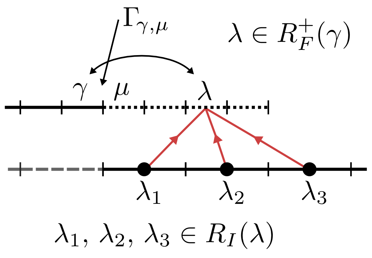
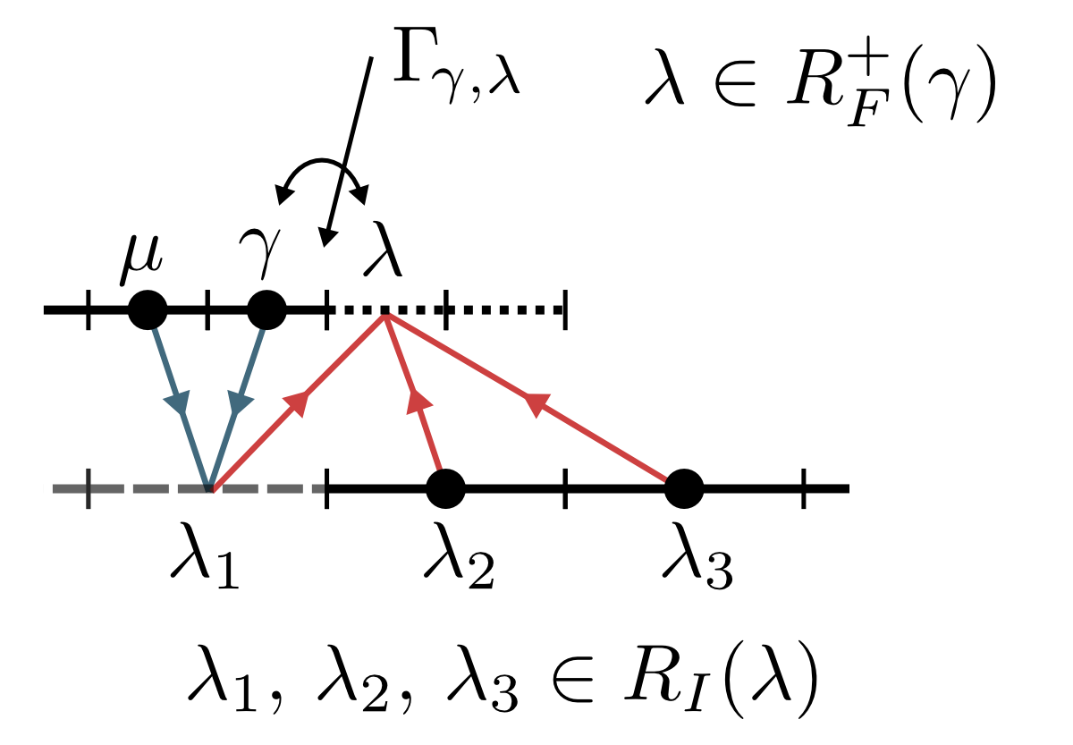
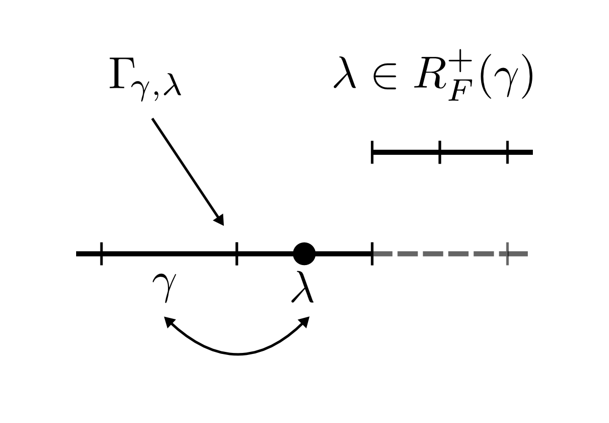
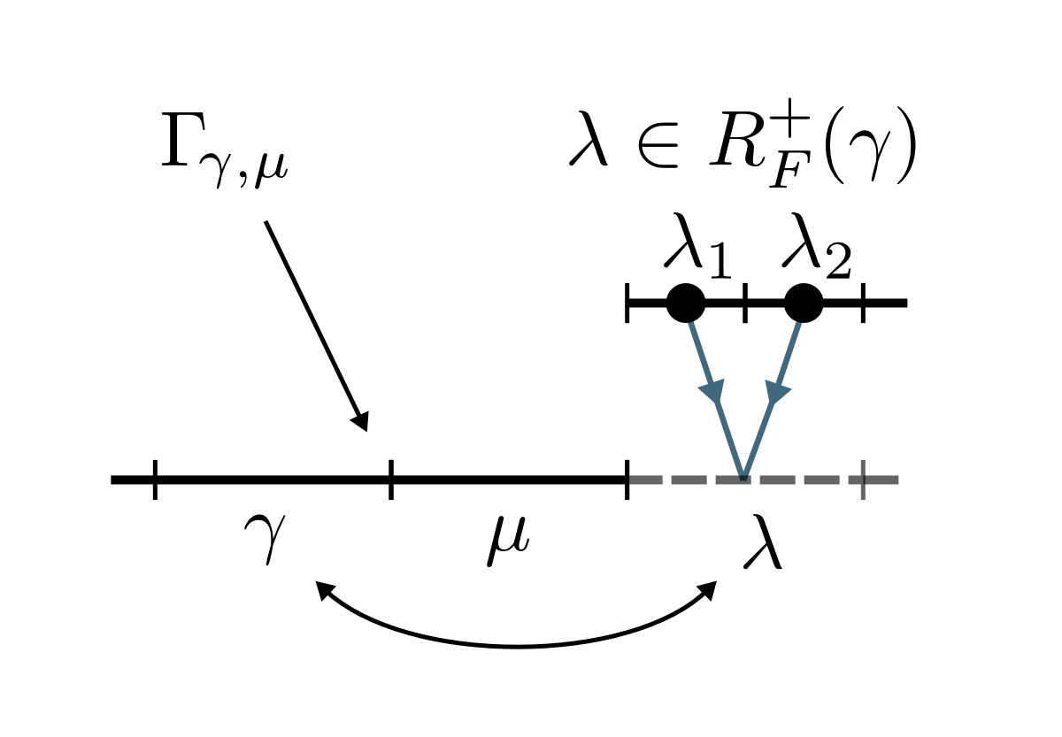
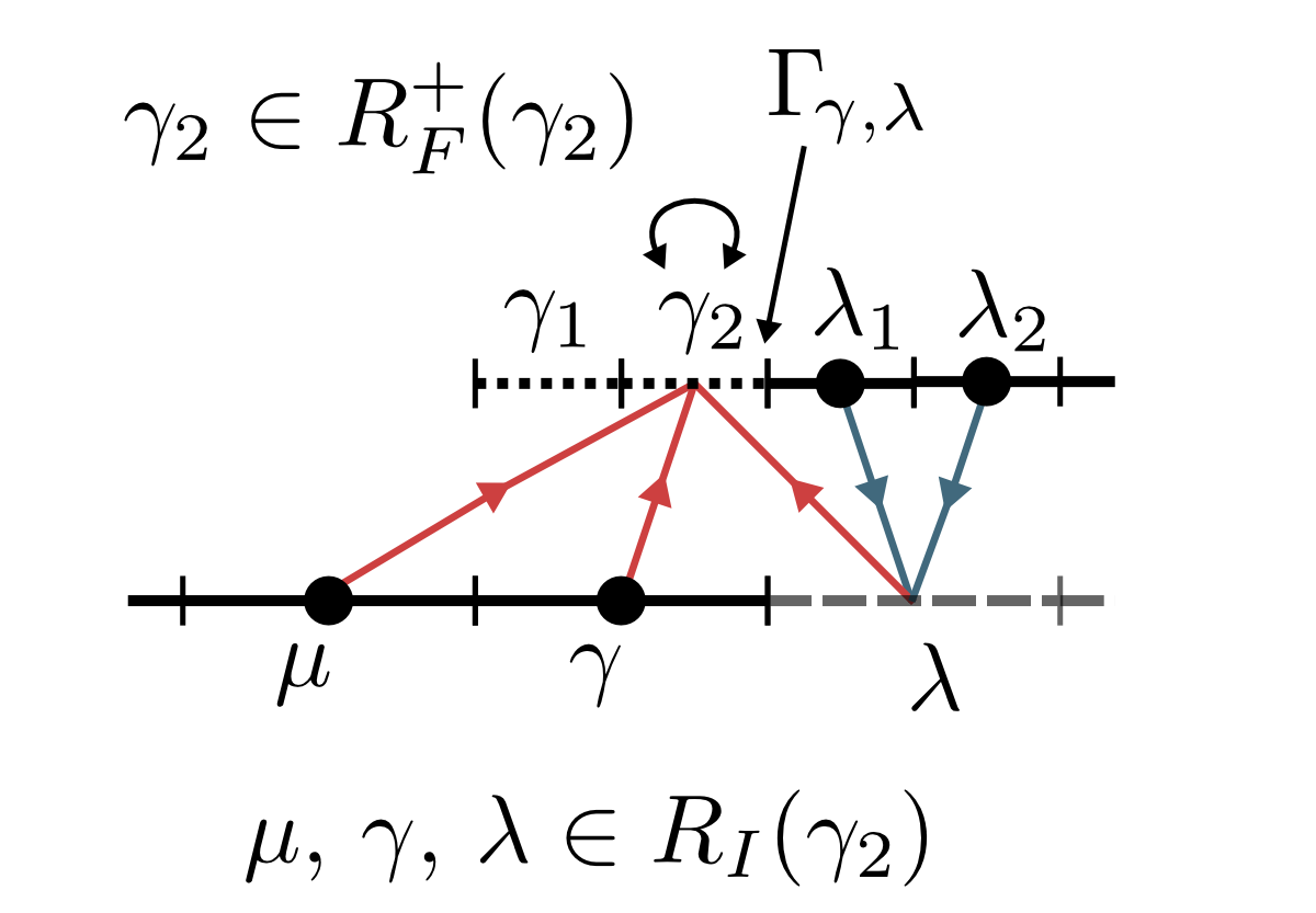
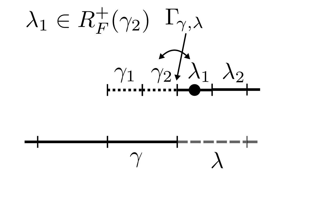
Given a certain leaf $\Omega_{\gamma}$, for each cell $\Omega_{\lambda}$ within the flux stencil $R^{+}_{F}(\gamma)$ ($\lambda\in R^{+}_{F}(\gamma)$) there are three cases:

1. Cell $\Omega_{\lambda}$ is a leaf and thus belongs to the adapted grid, i.e., $\lambda\in\bigcup_{r=1}^{N_{\rm R}}{\mathrm{L}}(\Lambda_{r})$. The coefficient $a_{h(\gamma),h(\lambda)}$ is computed according to (25) as for a uniform grid (see, for instance, Figure 2(a)).

2. Cell $\Omega_{\lambda}$ belongs to the set of adapted grids but it is not a leaf, i.e., $\lambda\in\bigcup_{r=1}^{N_{\rm R}}{\mathrm{T}}(\Lambda_{r})\wedge\lambda\notin\bigcup_{r=1}^{N_{\rm R}}{\mathrm{L}}(\Lambda_{r})$. In this case inner cells are linked to leaves using the projection operator (3). In Figure 2(b), (25) is replaced by

   $$a_{h(\gamma),h(\lambda_{i})}=a_{h(\gamma),h(\lambda_{i})}+|\Omega_{\lambda}|^{-1}|\Omega_{\lambda_{i}}|\alpha_{\gamma,\lambda},\qquad\Omega_{\lambda_{i}}\subset\Omega_{\lambda},i=1,2.$$

3. Cell $\Omega_{\lambda}$ is a phantom, i.e., $\lambda\in\bigcup_{r=1}^{N_{\rm R}}{\mathrm{P}}(\Lambda_{r})$. As established by (27), phantoms are linked to leaves and/or inner cells using the prediction operation (4). For Figure 2(c) we thus have

   $$a_{h(\gamma),h(\lambda_{i})}=a_{h(\gamma),h(\lambda_{i})}+\beta_{\lambda,\lambda_{i}}\alpha_{\gamma,\lambda},\qquad\lambda_{i}\in R_{I}(\lambda),i=1,2,3;$$

   whereas in Figure 2(d) $\Omega_{\lambda_{1}}$ is not a leaf and hence, $a_{h(\gamma),h(\lambda_{1})}$ must be replaced by

   $$a_{h(\gamma),h(\mu)}=a_{h(\gamma),h(\mu)}+|\Omega_{\lambda_{1}}|^{-1}|\Omega_{\mu}|\beta_{\lambda,\lambda_{1}}\alpha_{\gamma,\lambda},\qquad\Omega_{\mu}\subset\Omega_{\lambda_{1}},\lambda_{1}\in R_{I}(\lambda),$$

   $$a_{h(\gamma),h(\gamma)}=a_{h(\gamma),h(\gamma)}+|\Omega_{\lambda_{1}}|^{-1}|\Omega_{\gamma}|\beta_{\lambda,\lambda_{1}}\alpha_{\gamma,\lambda},\qquad\Omega_{\gamma}\subset\Omega_{\lambda_{1}},\lambda_{1}\in R_{I}(\lambda),$$

   combining both inter-level operations (3) and (4).

Additionally, if a leaf $\Omega_{\gamma}$ shares an interface $\Gamma_{\gamma,\lambda}$ with another of higher resolution, coefficients $\widetilde{a}_{h(\gamma),l}$ are computed at grid-level $|\gamma|+1$, considering the corresponding phantoms, children of $\Omega_{\gamma}$, at $\Gamma_{\gamma,\lambda}$. For instance, when considering the interface $\Gamma_{\gamma,\lambda}$ in Figure 3, the stencil $R^{+}_{F}(\gamma_{2})$ is considered corresponding to the phantom $\Omega_{\gamma_{2}}$, child of $\Omega_{\gamma}$. For $\Omega_{\gamma_{2}}$ contained in $R^{+}_{F}(\gamma_{2})$ (Figure 3(a)), we thus have

$$a_{h(\gamma),h(\mu)}=a_{h(\gamma),h(\mu)}+|\Omega_{\gamma}|^{-1}|\Omega_{\gamma_{2}}|\beta_{\gamma_{2},\mu}\alpha_{\gamma_{2},\gamma_{2}},\qquad \Omega_{\gamma_{2}}\subset\Omega_{\gamma},\mu\in R_{I}(\gamma_{2}),$$

$$a_{h(\gamma),h(\gamma)}=a_{h(\gamma),h(\gamma)}+|\Omega_{\gamma}|^{-1}|\Omega_{\gamma_{2}}|\beta_{\gamma_{2},\gamma}\alpha_{\gamma_{2},\gamma_{2}},\qquad \Omega_{\gamma_{2}}\subset\Omega_{\gamma},\gamma\in R_{I}(\gamma_{2}),$$

$$a_{h(\gamma),h(\lambda_{i})}=a_{h(\gamma),h(\lambda_{i})}+|\Omega_{\gamma}|^{-1}|\Omega_{\gamma_{2}}|\beta_{\gamma_{2},\lambda}|\Omega_{\lambda}|^{-1}|\Omega_{\lambda_{i}}|\alpha_{\gamma_{2},\gamma_{2}},\qquad \Omega_{\gamma_{2}}\subset\Omega_{\gamma},\lambda\in R_{I}(\gamma_{2}),\Omega_{\lambda_{i}}\subset\Omega_{\lambda},i=1,2;$$

whereas for $\Omega_{\lambda_{1}}$, also contained in $R^{+}_{F}(\gamma_{2})$ (Figure 3(b)):

$$a_{h(\gamma),h(\lambda_{1})}=a_{h(\gamma),h(\lambda_{1})}+|\Omega_{\gamma}|^{-1}|\Omega_{\gamma_{2}}|\alpha_{\gamma_{2},\lambda_{1}},\qquad\Omega_{\gamma_{2}}\subset\Omega_{\gamma}.$$

(a)                                                                 (b)

Figure 3: Computation of coefficients at inter-grid interfaces when a leaf $\Omega_{\gamma}$ shares an interface with another one of higher resolution. Leaves, inner cells, and phantoms are represented with solid, dashed, and dotted lines, respectively. Coefficients related to cell $\Omega_{\gamma}$ (a) and $\Omega_{\lambda_{1}}$ (b) are written in terms of leaves marked with $\bullet$.

The general, multi-dimensional scheme to construct the discrete Laplacian is detailed for the sake of completeness in Appendix B. The algorithm (with computational complexity ${\mathcal{O}}(N_{\rm L})$) considers multiplications and combinations of constant coefficients coming from the finite volume discretization and the inter-level multiresolution operations as previously shown. The operator $\mathbf{\widetilde{A}}$ is thus represented directly on the adapted grid strongly coupling consistent inter-grid and conservation properties. In this study we do not develop our own linear solver to solve the discrete Poisson equation. We rather rely on dedicated solvers available in the literature whose performance to solve multidimensional linear systems have already been demonstrated. Consequently, matrix $\mathbf{\widetilde{A}}$ must be an input to these solvers; otherwise, the same operations described here would have been performed without having to save the matrix entries in memory. Here operator $\mathbf{\widetilde{A}}$ is stored using a standard CSR (Compressed Sparse Row) format for sparse matrices.

4 Streamer discharge simulations

Classical fluid model for streamers in air at atmospheric pressure is given by drift-diffusion equations consistently coupled with a Poisson equation [4, 37]:

$$\left.\begin{array}[]{l}\partial_{t}n_{\rm e}+\partial_{\boldsymbol{x}}\cdot(n_{\rm e}\,{\boldsymbol{v}}_{\!\rm e})-\partial_{\boldsymbol{x}}\cdot(D_{\rm e}\ \partial_{\boldsymbol{x}}n_{\rm e})=n_{\rm e}\nu_{\rm i}-n_{\rm e}(\nu_{{\rm a}2}+\nu_{{\rm a}3})-n_{\rm e}n_{\rm p}\beta_{\rm ep}+n_{\rm n}\gamma+S_{\rm ph},\\[6.45831pt] \partial_{t}n_{\rm p}+\partial_{\boldsymbol{x}}\cdot(n_{\rm p}{\boldsymbol{v}}_{\!\rm p})-\partial_{\boldsymbol{x}}\cdot(D_{\rm p}\,\partial_{\boldsymbol{x}}n_{\rm p})=n_{\rm e}\nu_{\rm i}-n_{\rm e}n_{\rm p}\beta_{\rm ep}-n_{\rm n}n_{\rm p}\beta_{\rm np}+S_{\rm ph},\\[6.45831pt] \partial_{t}n_{\rm n}+\partial_{\boldsymbol{x}}\cdot(n_{\rm n}{\boldsymbol{v}}_{\!\rm n})-\partial_{\boldsymbol{x}}\cdot(D_{\rm n}\,\partial_{\boldsymbol{x}}n_{\rm n})=n_{\rm e}(\nu_{{\rm a}2}+\nu_{{\rm a}3})-n_{\rm n}n_{\rm p}\beta_{\rm np}-n_{\rm n}\gamma,\end{array}\right\}$$ (28)

$$\varepsilon_{0}\,\partial_{\boldsymbol{x}}\cdot{\boldsymbol{E}}=-q_{\rm e}(n_{\rm p}-n_{\rm n}-n_{\rm e}),\quad{\boldsymbol{E}}=-\partial_{\boldsymbol{x}}\phi,$$ (29)

where ${\boldsymbol{x}}\in{\mathbb{R}}^{d}$, $n_{\rm i}$ is the density of charged species ${\rm i}$ (e: electrons, p: positive ions, n: negative ions), $\phi$ and ${\boldsymbol{E}}$ stand, respectively, for the electric potential and field, and ${\boldsymbol{v}}_{\rm i}=\mu_{\rm i}{\boldsymbol{E}}$ is the drift velocity. We denote by $D_{\rm i}$ and $\mu_{\rm i}$, respectively, the diffusion coefficient and the mobility of charged species ${\rm i}$, $q_{\rm e}$ is the absolute value of the electron charge, and $\varepsilon_{0}$ is the permittivity of free space. Moreover, $\nu_{\rm i}$ is the electron impact ionization coefficient, $\nu_{{\rm a}2}$ and $\nu_{{\rm a}3}$ are the two-body and three-body electron attachment coefficients, $\beta_{\rm ep}$ and $\beta_{\rm np}$ are, respectively, the electron-positive ion and negative-positive ion recombination coefficients, and $\gamma$ is the detachment coefficient. All these coefficients depend on the local reduced electric field $E/N_{\rm air}$ and thus vary in time and space, where $E=|{\boldsymbol{E}}|$ is the electric field magnitude and $N_{\rm air}$ is the air neutral density. For test studies presented in this paper, the transport parameters for air are taken from [44]; detachment and attachment coefficients, respectively, from [6, 36]; and other reaction rates, also from [44]. Diffusion coefficients for ions are derived from mobilities using classical Einstein relations. Our reference density for air is $N_{\rm air}=2.688\times 10^{19}\,$cm^-3.

For positive streamers a sufficient number of seed-electrons needs to be present in front of the streamer head as the direction of electron motion is opposed to the streamer propagation (see [11] and references therein). Photoionization is in general an accepted mechanism to produce such seed-electrons in nitrogen-oxygen mixtures. It is therefore introduced into the drift-diffusion system (28) as a source term ($S_{\rm ph}$) that needs to be evaluated in general at each time-step for all points of the computational domain. Computation of $S_{\rm ph}$ is detailed in Appendix C which requires the iterative solution of six elliptic equations given by (34) with boundary conditions (35). Iterating three times amounts then to solve 18 elliptic equations per time-step.

In what follows we will first assess the theoretical validity of the mathematical description conducted in §2.2 and the numerical implementation described in §3.2. This study will be conducted on a simplified multi-dimensional model with known analytical solution that mimics the spatial configuration typically found in streamer discharges. In a second part we will present two-dimensional double-headed streamer simulations modeled by (28)–(29), for which we will evaluate the performance of different linear solvers implemented to solve the discrete Poisson equations. Finally, dynamic grid adaptation will be analyzed for the numerical simulation of two interacting positive streamers in a two-dimensional configuration that leads to streamer merging.

4.1 Numerical validation

We first investigate the validity of bound (18) (and (19)). That is, the numerical error related to grid adaptation and data compression is of ${\mathcal{O}}(\eta_{\rm MR})$, where $\eta_{\rm MR}$ is a user-defined accuracy tolerance. Given a set of constant parameters: $a$, $b$, and $\sigma$, let us consider an exponential function $\phi({\boldsymbol{x}})$ on a multi-dimensional domain $\Omega\subset{\mathbb{R}}^{d}$,

$$\phi({\boldsymbol{x}})=g({\boldsymbol{x}})+b=a\exp\left(-|{\boldsymbol{x}}|^{2}/\sigma^{2}\right)+b,\quad{\boldsymbol{x}}\in\Omega$$ (30)

that verifies the following Poisson equation:

$$\partial_{\boldsymbol{x}}^{2}\phi({\boldsymbol{x}})=\rho({\boldsymbol{x}}),\quad\rho({\boldsymbol{x}})=\frac{4}{\sigma^{2}}\left(\frac{|{\boldsymbol{x}}|^{2}}{\sigma^{2}}-1\right)g({\boldsymbol{x}}),\quad{\boldsymbol{x}}\in\Omega,$$ (31)

with boundary conditions,

$$\phi({\boldsymbol{x}})=g({\boldsymbol{x}})+b,\quad{\boldsymbol{x}}\in\partial\Omega.$$ (32)

Using the standard, second-order centered scheme (similar to (22)), we discretize equation (31) on a two- and a three-dimensional region: $[-0.5,0.5]^{2}$ and $[-0.5,0.5]^{3}$, respectively, and we consider the set of parameters: $a=10$, $b=20$, and $\sigma=0.005$. The value of $\sigma$ has been chosen such that function $\rho({\boldsymbol{x}})$ exhibits similar steep gradients as those found in a developed streamer head modeled by (28)–(29). Since $g({\boldsymbol{x}})$ decays rapidly toward the boundaries, we consider Dirichlet boundary conditions in (32): $\phi({\boldsymbol{x}})=b$, whereas symmetric boundary conditions are taken in order to consider a reduced two- and a three-dimensional computational domain: $[-0.5,0.5]\times[0,0.5]$ and $[0,0.5]^{3}$, respectively.

Figure 4: $L^{2}$-errors between analytical and numerical solutions $\phi$ of Poisson equation (31) (a) and component $E_{x}$ of ${\boldsymbol{E}}=-\partial_{\boldsymbol{x}}\phi$ (b) for several threshold values $\eta_{\rm MR}$ ( $\eta_{\rm MR}=10^{-4}$ for the three-dimensional problem).

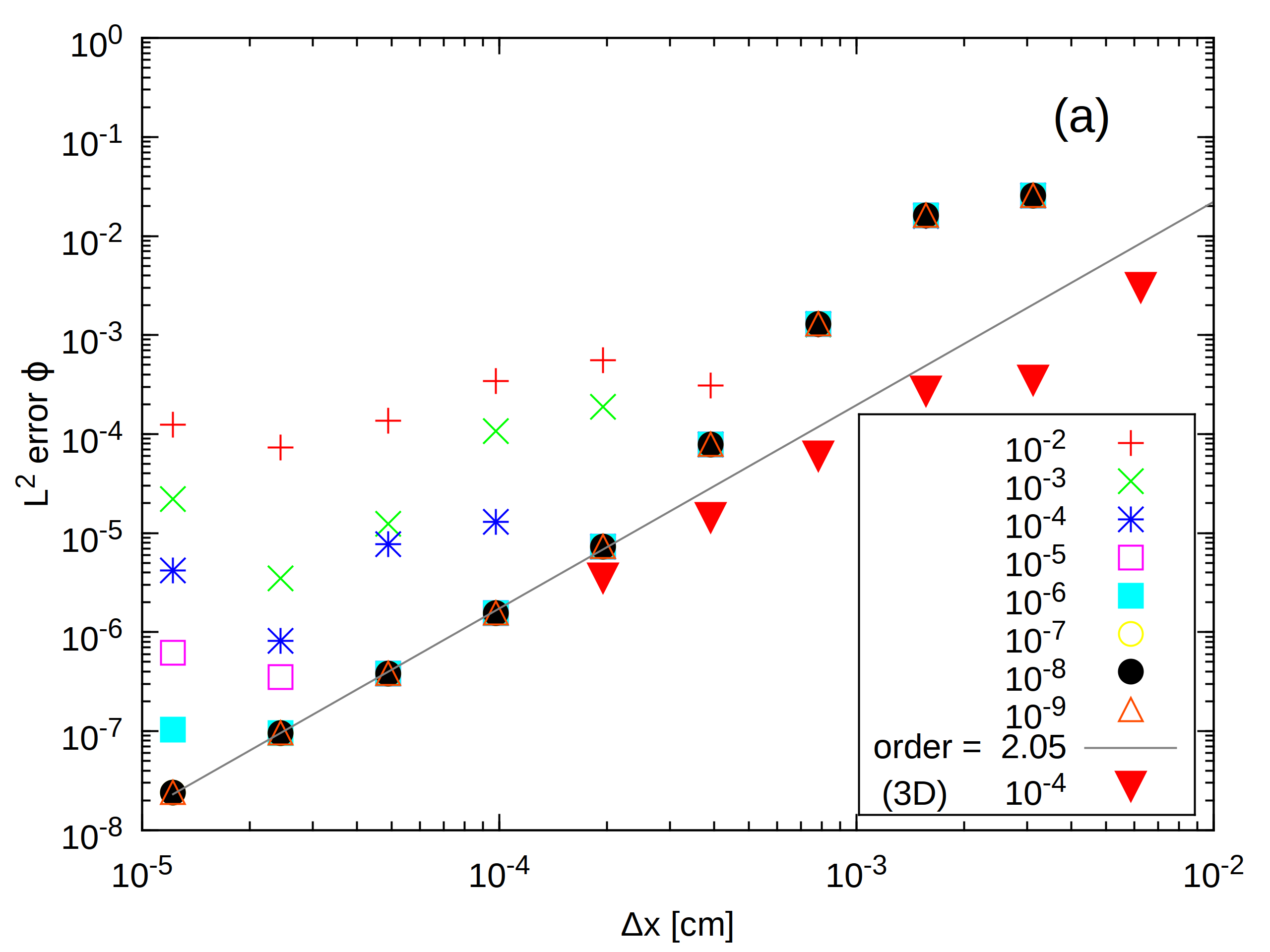
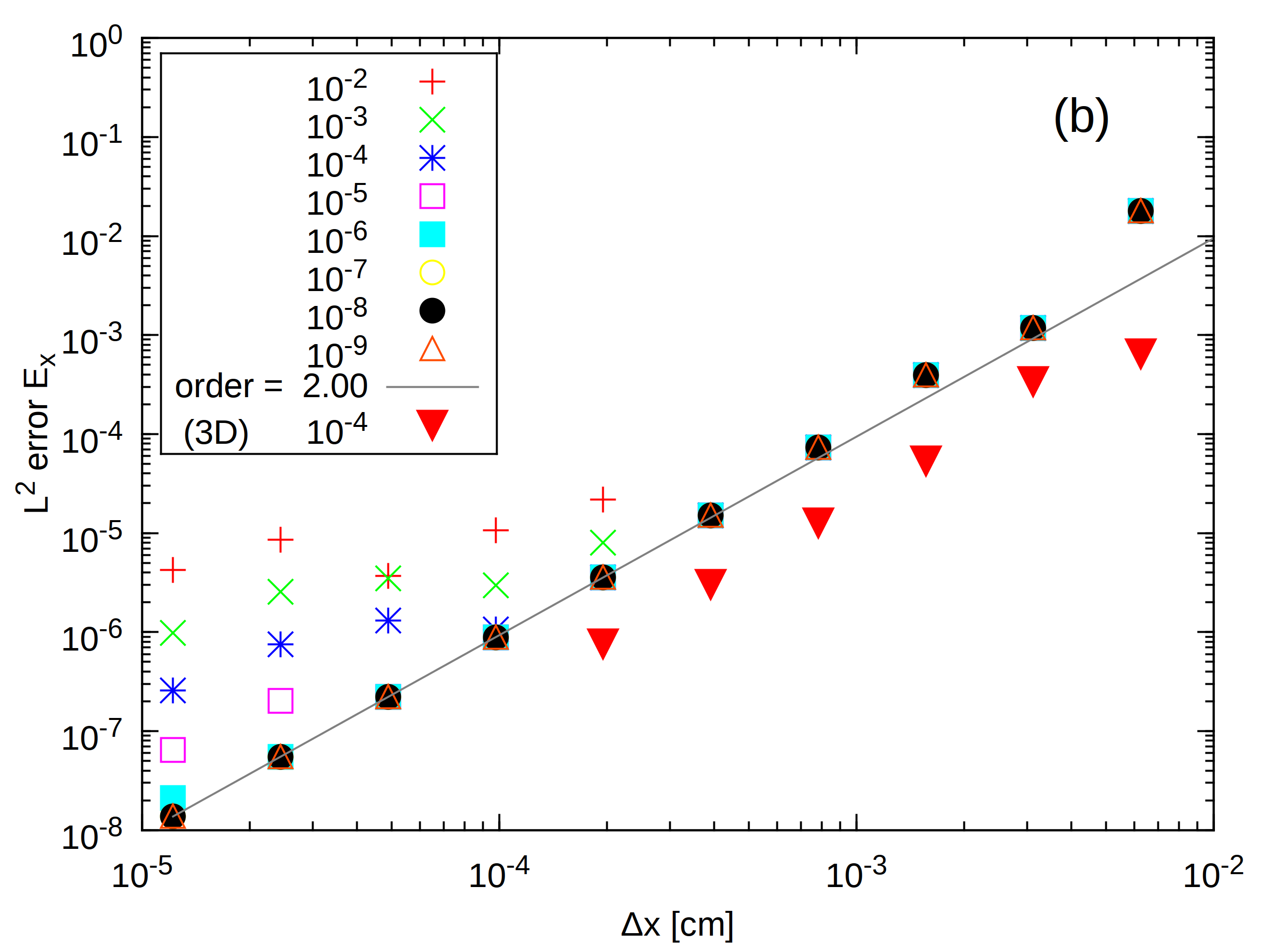
Figure 4 shows normalized $L^{2}$-errors between the analytical solution (30) and the numerical solution of the Poisson equation (31) discretized on an adapted grid, obtained with several threshold values $\eta_{\rm MR}$. The resulting linear systems were solved using MUMPS [3, 2], a direct linear system solver, and BoomerAMG [34] (contained in the hypre library), an iterative solver, for the two- and three-dimensional problems, respectively. The finest spatial discretization is denoted by $\Delta x$, and it is set by the choice of the maximum level $J$ in the multiresolution analysis and the number of roots per direction: $N_{{\rm R}x}$, $N_{{\rm R}y}$, and $N_{{\rm R}z}$. For the two-dimensional case, $\Delta x=1/(N_{{\rm R}x}2^{J})$ with $J=5,6,\ldots,13$, $N_{{\rm R}x}=10$, and $N_{{\rm R}y}=5$; whereas for the three-dimensional one: $\Delta x=0.5/(N_{{\rm R}x}2^{J})$ with $J=4,5,\ldots,9$, $N_{{\rm R}x}=N_{{\rm R}y}=N_{{\rm R}z}=5$. All computations were performed on a work station with 24 GB of computer memory. For streamer discharge simulations an accurate resolution of the electric field: ${\boldsymbol{E}}=-\partial_{\boldsymbol{x}}\phi$, is essential for good physical descriptions. Therefore, we have also computed ${\boldsymbol{E}}$ with a second-order, centered approximation, and compared it against its analytical counterpart: ${\boldsymbol{E}}=2{\boldsymbol{x}}\,g({\boldsymbol{x}})/\sigma^{2}$. In both cases, for $\phi$ and ${\boldsymbol{E}}$, the numerical errors behave like a second order spatial approximation even if the solutions are computed on an adapted grid, especially for relatively coarse discretizations or sufficiently fine multiresolution threshold values. For finer resolutions, the numerical errors coming from the adaptive multiresolution become more dominant and the numerical errors are effectively bounded by the threshold parameter $\eta_{\rm MR}$. Bounds (18) and (19) prove then to describe accurately the behavior of the numerical approximations when solving a Poisson equation on a multiresolution adapted grid.

Figure 5: Matrix construction and solution: (a) discrete Laplacian $\mathbf{\widetilde{A}}$ on a two-dimensional multiresolution grid; and (b) CPU times to build $\mathbf{\widetilde{A}}$ and solve the corresponding linear systems for several numbers of cells (slopes of data fits are indicated).

Figure 6: Discrete Laplacian $\mathbf{\widetilde{A}}$ on a three-dimensional multiresolution grid (a); and (b) cutting planes through the adapted mesh for $J=9$, $N_{{\rm R}x}=N_{{\rm R}y}=N_{{\rm R}z}=5$, and $\eta_{\rm MR}=10^{-4}$.

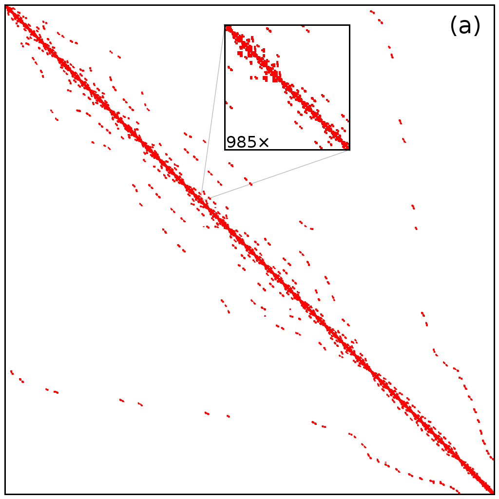
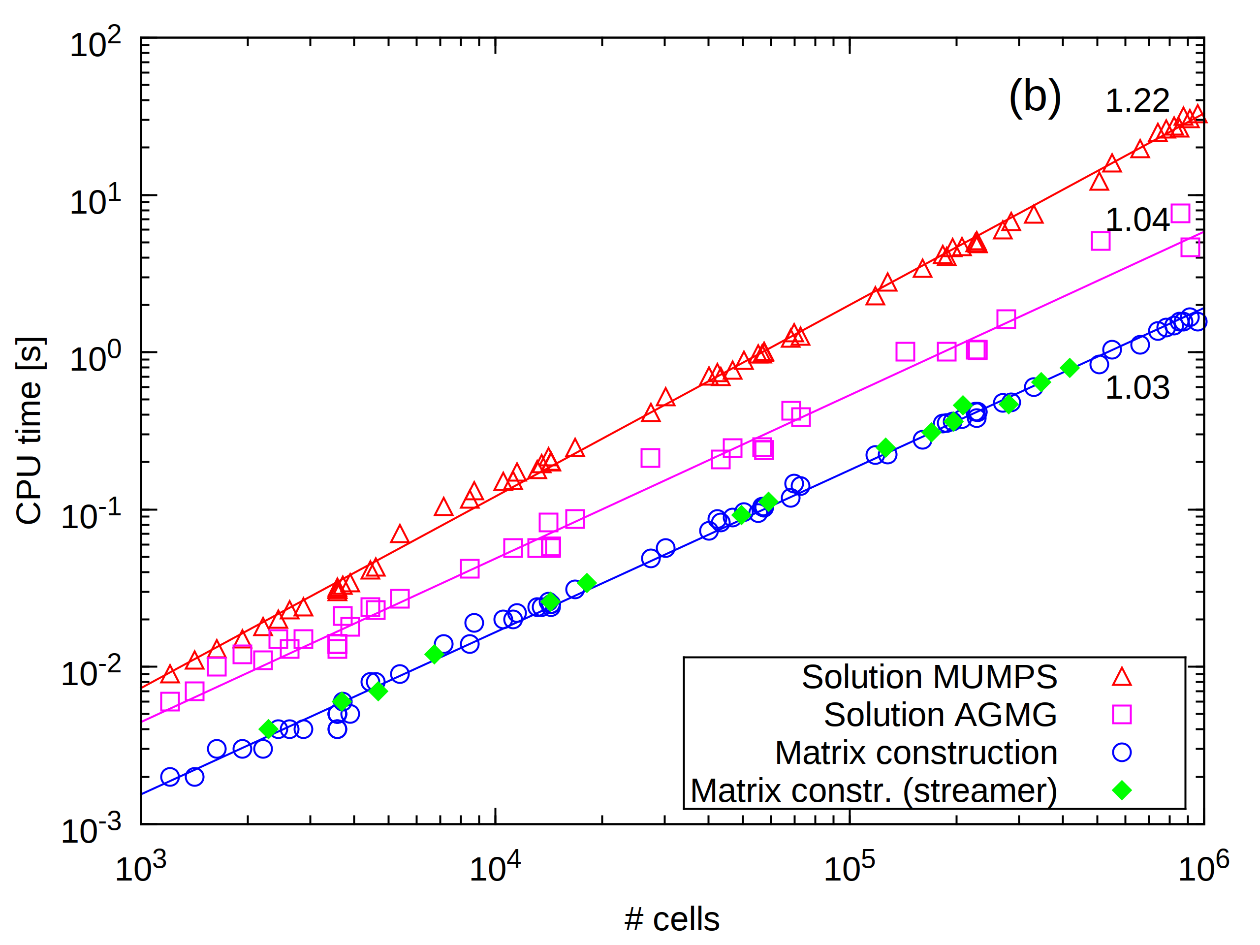
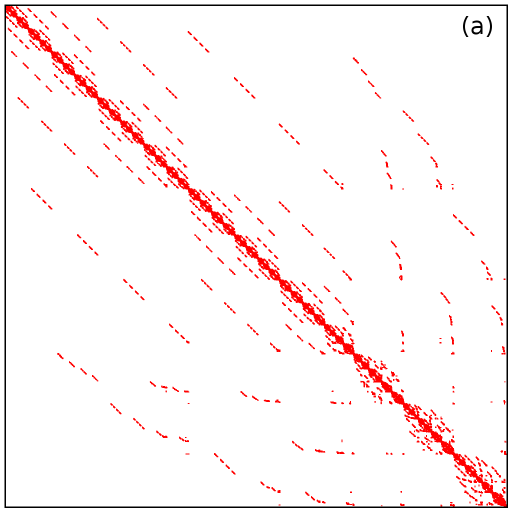
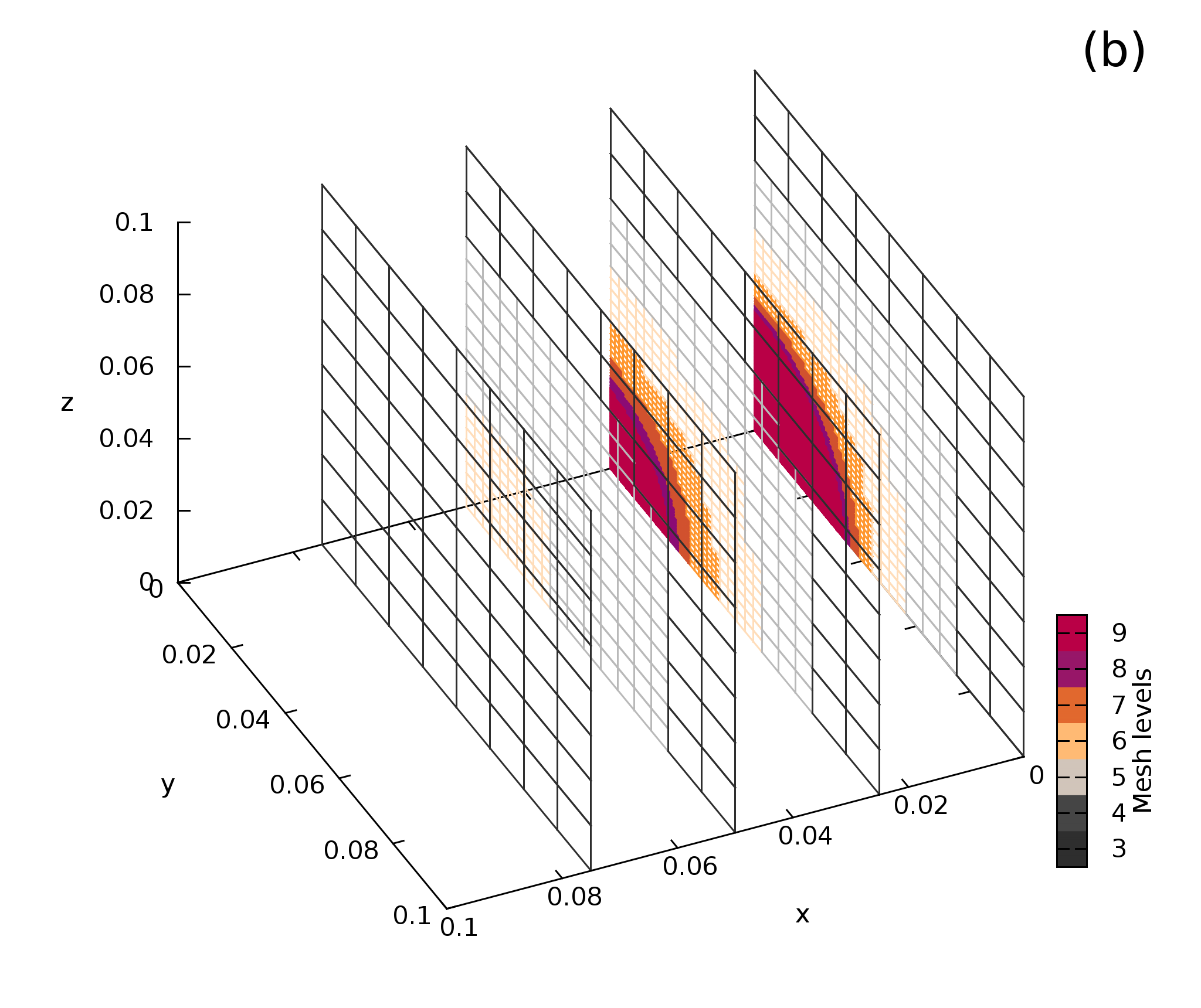
These tests allow us to verify that the discrete Laplacian is consistently constructed following the procedure established in §3.2, and correctly implemented in practice. The matrix representation $\mathbf{\widetilde{A}}$ is shown in Figure 5(a) (recall that only non-zero entries are actually saved in memory). Notice that matrix $\mathbf{\widetilde{A}}$ cannot be symmetric, unless no grid adaptation is performed. However, $\mathbf{\widetilde{A}}$ is in general quasi-symmetric. For instance, for this particular problem approximately $89\,$% of symmetry is retrieved in terms of non-zero elements of the matrix. Figure 5(b) illustrates the computational complexity of the matrix construction, which behaves like ${\mathcal{O}}(N_{\rm L})$. The different measures were obtained performing several computations with different finest grid-levels $J\in[9,\ldots,13]$, and multiresolution parameters $\eta_{\rm MR}\in[10^{-2},\ldots,10^{-9}]$. We have indicated in Figure 5(b) the CPU times to solve the resulting linear system with MUMPS, as well as with an algebraic multigrid solver: AGMG [49, 47, 50] (tolerances set to $10^{-9}$), of a computational complexity of ${\mathcal{O}}(N_{\rm L})$. We have also verified that building the matrix representation behaves the same way for the more complex streamer configuration presented in the following. Finally, Figure 6(a) shows operator $\mathbf{\widetilde{A}}$ on a three-dimensional adapted grid. As an illustration, the number of non-zero entries is $29756821$ for $2846787$ cells on the adapted grid (a ratio of about $10.5$) with $68\,$% of symmetry. The adapted grid for the finest three-dimensional configuration is shown in Figure 6(b), corresponding to an equivalent uniform grid of $5^{3}\times 512^{3}$ for $J=9$ and $N_{{\rm R}x}=N_{{\rm R}y}=N_{{\rm R}z}=5$.

4.2 Performance of linear solvers

We present a brief study on the performance of several software packages currently available in the literature to solve linear systems of general type: $\mathbf{A}\mathbf{x}=\mathbf{b}$. Our attention will be focused on iterative solver, which in general exhibit relatively modest memory requirements with respect to direct ones. In particular algebraic multigrid methods (AMG) will be investigated. These methods do not require an explicit grid geometry and work directly on matrix entries; they are therefore well-suited to our purposes since system $\mathbf{A}\mathbf{x}=\mathbf{b}$, stemmed in our case from the discretization of a Poisson equation on a multiresolution adapted grid, has completely lost any reminiscence of its original geometric layout.

4.2.1 Test configuration

Let us consider the propagation of a two-dimensional double-headed streamer at atmospheric pressure. In this configuration positive and negative streamers emerge from an initial germ of charged species. Drift-diffusion equations (28) together with Poisson equation (29) are solved following the time-space adaptive scheme introduced in [26]. The latter is based on a decoupled numerical solution of (28) and (29) in such a way that each problem is solved separately by a dedicated solver. Both numerical approximations are assembled according to a second order scheme in time. The latter also considers a time-stepping procedure with error control such that a prescribed accuracy $\eta_{\mathcal{T}}$ is attained. Variables are represented at cell centers except for the electric field and the velocities which are staggered, while the entire problem is solved on an adapted grid dynamically obtained by multiresolution analysis. The latter is performed on the species densities. Notice that the right-hand side of the Poisson equation (29) is a linear combination of these variables; hence, the theoretical framework in §2.2 remains valid.

Numerical simulations in the present study were carried out with a space-time accuracy tolerance of $\eta_{\rm MR}=\eta_{\mathcal{T}}=10^{-4}$ with a space resolution of 3.9$\,\mu$m corresponding to a finest grid level: $J=8$ with $N_{{\rm R}x}=10$ and $N_{{\rm R}y}=3$. This set of parameters guarantees a sufficiently fine time-space representation of the physics, and numerical results disclosing practically the same behavior with higher spatial resolutions and tighter accuracy tolerances. The computational domain is given by $[-0.5,0.5]\times[0,0.3]\,$cm in a Cartesian configuration. A homogeneous electric field ${\boldsymbol{E}}=(48.0,0)\,$kV/cm is introduced via Dirichlet boundary conditions for the Poisson equation at $x=\pm 0.5\,$cm, whilst Neumann boundary conditions are applied at $y=0.3\,$cm. A plane of symmetry is imposed at $y=0$, thus only one half of the streamer is actually simulated. The double-headed streamer is initiated by placing a Gaussian plasma cloud so that the initial conditions for the transport equations (28) are given by

$$n_{\rm p}({\boldsymbol{x}},0)=n_{\rm e}({\boldsymbol{x}},0)=n_{\max}\exp\left(-|{\boldsymbol{x}}|^{2}/\sigma^{2}\right)+n_{0{\rm p,e}},\quad n_{\rm n}({\boldsymbol{x}},0)=n_{0{\rm n}},$$

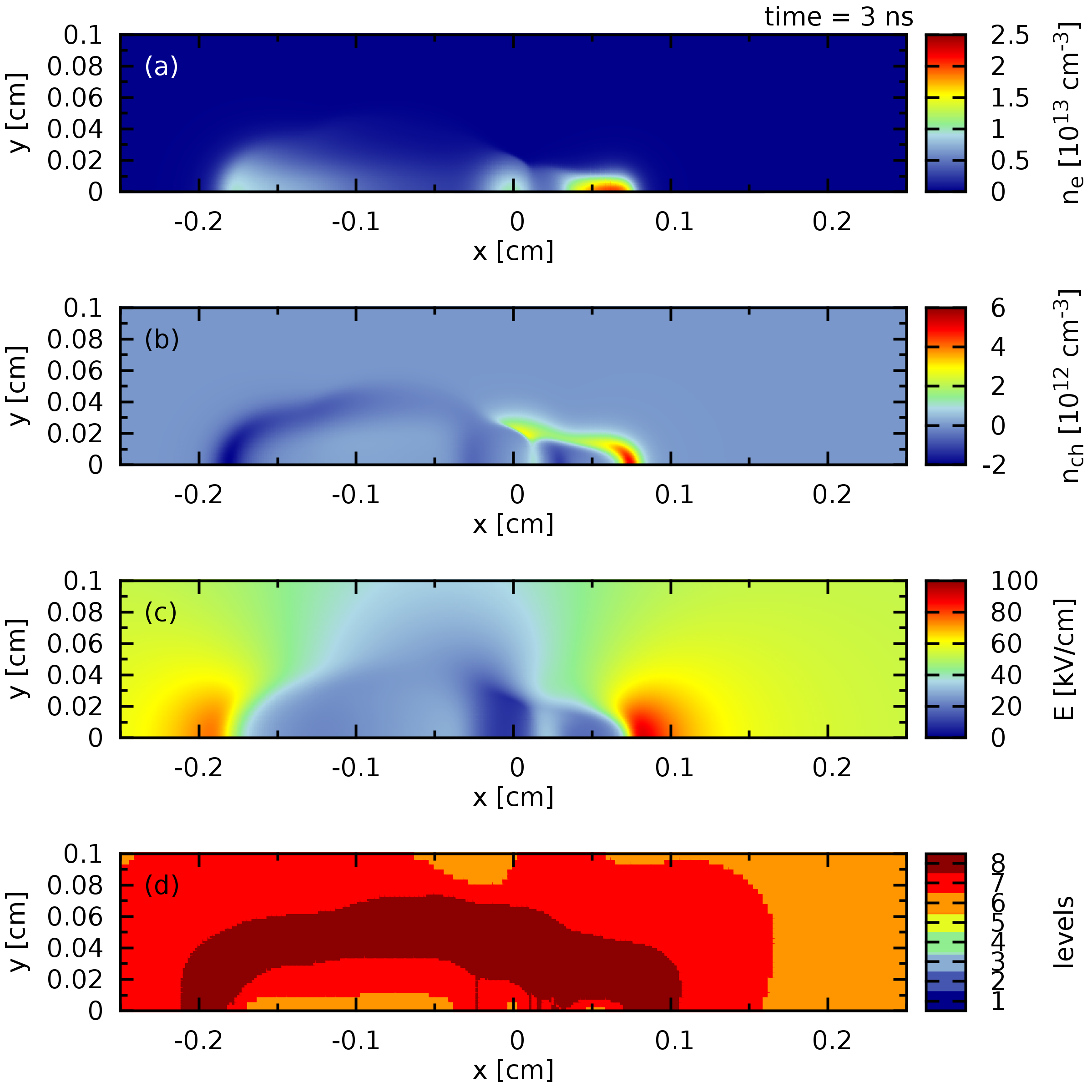
with $\sigma=0.02\,$cm, $n_{\max}=10^{13}\,$cm^-3, and a small homogeneous pre-ionization background of $n_{0{\rm n,e}}=5\times 10^{-5}\,$cm^-3 and $n_{0{\rm p}}=10^{-4}\,$cm^-3. All tests were conducted starting from the same solution at $3.0\,$ns when the double-headed streamer is already well developed but no interference with the boundaries is evidenced. The electron density, the net charge species density: $n_{\rm ch}=n_{\rm p}-n_{\rm n}-n_{\rm e}$, the magnitude of the electric field, and the levels of the adapted grid at $3.0\,$ns are shown in Figure 7. The total number of cells is of $197784$, distributed over five grid-levels from a resolution of 62.5$\,\mu$m at level $j=4$ up to 3.9$\,\mu$m at $J=8$. A data compression of about $10\,$% is thus achieved with respect to a uniform grid with the finest spatial resolution.

Figure 7: Double-headed streamer at $3.0\,$ns: (a) electron density $n_{\rm e}$; (b) net charged-species density $n_{\rm ch}$; (c) magnitude of the electric field $E=|{\boldsymbol{E}}|$; and (d) grid-levels of the adapted mesh. Only part of the computational domain is shown.

Table 1: Iterative solvers: number of iterations (#iter) for relative tolerances: $tol=10^{-6},\ldots,10^{-14}$, CPU computing time, $L^{2}$-error of $\phi$ and $|{\boldsymbol{E}}|$ with respect to solutions computed with MUMPS, and memory requirements for each solver.

AGMG										Memory: 82 MB
	$tol$			#iter			CPU(s)			$L^{2}$-error $\phi$			$L^{2}$-error $|{\boldsymbol{E}}|$
	$10^{-6}$			3			0.50			1.65$\times 10^{-5}$			1.40$\times 10^{-4}$
	$10^{-7}$			4			0.55			1.20$\times 10^{-5}$			2.94$\times 10^{-5}$
	$10^{-8}$			8			0.78			1.80$\times 10^{-6}$			4.20$\times 10^{-6}$
	$10^{-9}$			10			0.89			1.43$\times 10^{-7}$			4.10$\times 10^{-7}$
	$10^{-10}$			14			1.10			2.03$\times 10^{-8}$			4.74$\times 10^{-8}$
	$10^{-11}$			16			1.21			2.24$\times 10^{-9}$			7.44$\times 10^{-9}$
	$10^{-12}$			19			1.38			2.09$\times 10^{-11}$			9.65$\times 10^{-11}$
	$10^{-13}$			20			1.43			1.28$\times 10^{-11}$			3.68$\times 10^{-11}$
	$10^{-14}$			24			1.64			1.59$\times 10^{-12}$			3.86$\times 10^{-12}$
hypre BoomerAMG										Memory: 100 MB
	$tol$			#iter			CPU(s)			$L^{2}$ error $\phi$			$L^{2}$ error $|{\boldsymbol{E}}|$
	$10^{-6}$			3			1.23			7.36$\times 10^{-4}$			2.46$\times 10^{-3}$
	$10^{-7}$			6			1.51			1.81$\times 10^{-5}$			5.99$\times 10^{-5}$
	$10^{-8}$			8			1.71			3.97$\times 10^{-6}$			1.63$\times 10^{-5}$
	$10^{-9}$			11			1.98			9.56$\times 10^{-8}$			7.44$\times 10^{-7}$
	$10^{-10}$			14			2.27			9.04$\times 10^{-9}$			9.87$\times 10^{-8}$
	$10^{-11}$			17			2.55			5.45$\times 10^{-10}$			5.18$\times 10^{-9}$
	$10^{-12}$			20			2.83			6.24$\times 10^{-11}$			1.02$\times 10^{-9}$
	$10^{-13}$			24			3.21			6.28$\times 10^{-12}$			2.58$\times 10^{-11}$
	$10^{-14}$			27			3.52			4.73$\times 10^{-13}$			3.84$\times 10^{-12}$
hypre BoomerAMG + GMRES										Memory: 146 MB
	$tol$			#iter			CPU(s)			$L^{2}$ error $\phi$			$L^{2}$ error $|{\boldsymbol{E}}|$
	$10^{-6}$			2			1.24			9.09$\times 10^{-4}$			2.36$\times 10^{-3}$
	$10^{-7}$			5			1.57			2.65$\times 10^{-5}$			1.28$\times 10^{-4}$
	$10^{-8}$			8			1.90			1.15$\times 10^{-6}$			1.49$\times 10^{-5}$
	$10^{-9}$			10			2.13			6.19$\times 10^{-8}$			8.56$\times 10^{-7}$
	$10^{-10}$			12			2.34			4.32$\times 10^{-9}$			6.09$\times 10^{-8}$
	$10^{-11}$			14			2.58			5.77$\times 10^{-10}$			3.33$\times 10^{-9}$
	$10^{-12}$			15			2.69			3.58$\times 10^{-10}$			8.20$\times 10^{-10}$
	$10^{-13}$			17			2.93			3.57$\times 10^{-11}$			7.10$\times 10^{-11}$
	$10^{-14}$			19			3.15			3.13$\times 10^{-12}$			7.73$\times 10^{-12}$

4.2.2 Analysis of results

We have considered some iterative solvers readily available in various software packages. Most of present day linear solvers are developed with a special attention on enhanced parallel capabilities. Nevertheless, thanks to significant data compression achieved by multiresolution adaptation, the linear systems under consideration have typically about $10^{5}$ unknowns with approximately $10^{6}$ non-zero elements in the system matrix. Therefore, to simplify our study we have focused our attention on sequential performance of these solvers. We have performed the numerical experiments on a two-processor computer. Each processor is an Intel Xeon CPU E5410 @ 2.33GHz with a total available computer memory of 24 GB. The computer runs on a 64-bit version of Fedora 18 GNU/Linux system. All codes with the various linear solvers were compiled using compilers from GCC (version 4.7.2). Memory requirements of each solver were obtained by tracing the memory profiles of running programs with top command, executed in batch mode with a delay-time interval set to $0.01\,$s. In order to discriminate memory requirements for the linear solvers from the overall program memory usage, a reference program was executed in which calls to the solver were replaced by FORTRAN (GNU extension) SLEEP command.

The total number of unknowns for the Poisson equations considered in this problem is given by the number of cells in the adapted grid, $197784$ in this case, while the discrete Laplacian has $1078534$ non-zero entries (a ratio of about $5.5$). In what follows we consider as reference solution the solution to the Poisson equation (29): $\phi$, computed with MUMPS. For this problem, MUMPS requires $193\,$MB of memory space for a computation that takes approximately $3.96\,$s. As before we also analyze the approximation to the electric field: ${\boldsymbol{E}}=-\partial_{\boldsymbol{x}}\phi$. Data for three iterative solvers are presented in Table 1 for two algebraic multigrid solvers: AGMG and BoomerAMG, and for GMRES [53] preconditioned with BoomerAMG (also contained in hypre ). In all cases a fine-tuning of computing parameters have been previously carried out so that Table 1 includes the best performances obtained with each of these solvers for this particular problem. A key parameter for iterative solvers is given by the relative and absolute tolerances that in particular serve as stopping criteria to the iterative procedures. In this study we have set both tolerances equal to an accuracy tolerance, denoted as $tol$. The initial guess corresponds to the solution computed during the previous time-step. For tolerances higher or equal to $10^{-5}$ convergence is attained right-away with the initial guess for all three solvers. In all cases better performances are obtained with these iterative solvers with respect to MUMPS even with very fine accuracy tolerances $tol$. Even though GMRES converges in a less number of iterations for different values of $tol$ with respect to the algebraic multigrid solvers, it does not yield faster computations taking into account that for this problem preconditioning is the most expensive part. Therefore, BoomerAMG and GMRES/BoomerAMG require similar computing times.

With respect to the reference solution, all these iterative solvers scale well in terms of the accuracy of the approximations, set by the tolerance parameter $tol$. Notice that numerical errors related to iterative solvers must be taken into account to track the overall numerical accuracy of the simulation. In particular these numerical errors must be smaller than the multiresolution ones so that (18) and (19) remain valid. The latter could be enforced by setting in general: $tol<\eta_{\rm MR}$, while in this particular case a safer choice might be given by $tol\leq 10^{-3}\times\eta_{\rm MR}$ according to the values contained in Table 1. Among the solvers tested in this study, AGMG revealed itself as the most performing package both in terms of CPU time and memory requirements to solve this particular problem. However, the overall performance of these solvers is clearly problem-dependent. In this regard the hypre library provides a user-friendly and unified interface to various solution schemes, very appropriate to handle different types of problems.

4.3 Application to the study of two interacting positive streamers

While previous illustrations served to validate the numerical strategy, we consider now an interesting plasma physics application with more complex dynamics. We study the interaction of two positive streamers initiated to develop side by side. Because the heads of both streamers carry space charge of the same polarity, their mutual interaction should essentially be an electrostatic repulsion. However, it was found that streamers in such a configuration may attract each other and eventually merge [12, 22, 48]. This attraction is mainly the result of the enhancement of photoionization source in the space between the streamer heads [41, 10]. In particular, based on an extensive parametric numerical study, we have shown in [10] that for initial separations of two streamers smaller or comparable to the absorption length of photoionization, merging will start when the ratio of the streamer characteristic width and their mutual separation attains a certain value. We describe here some numerical aspects omitted in our previous study.

   

Figure 8: Time evolution of the net charge density (a), magnitude of the electric field (b), and dynamic grid adaptation (c) for two interacting positive streamers at ground pressure with an applied electric field of ${\boldsymbol{E}}_{\rm bg}=(0,-48)\,$kV/cm at time instances: $4.0$, $6.0$ and $8.0\,$ns. Only part of the computational domain is shown.

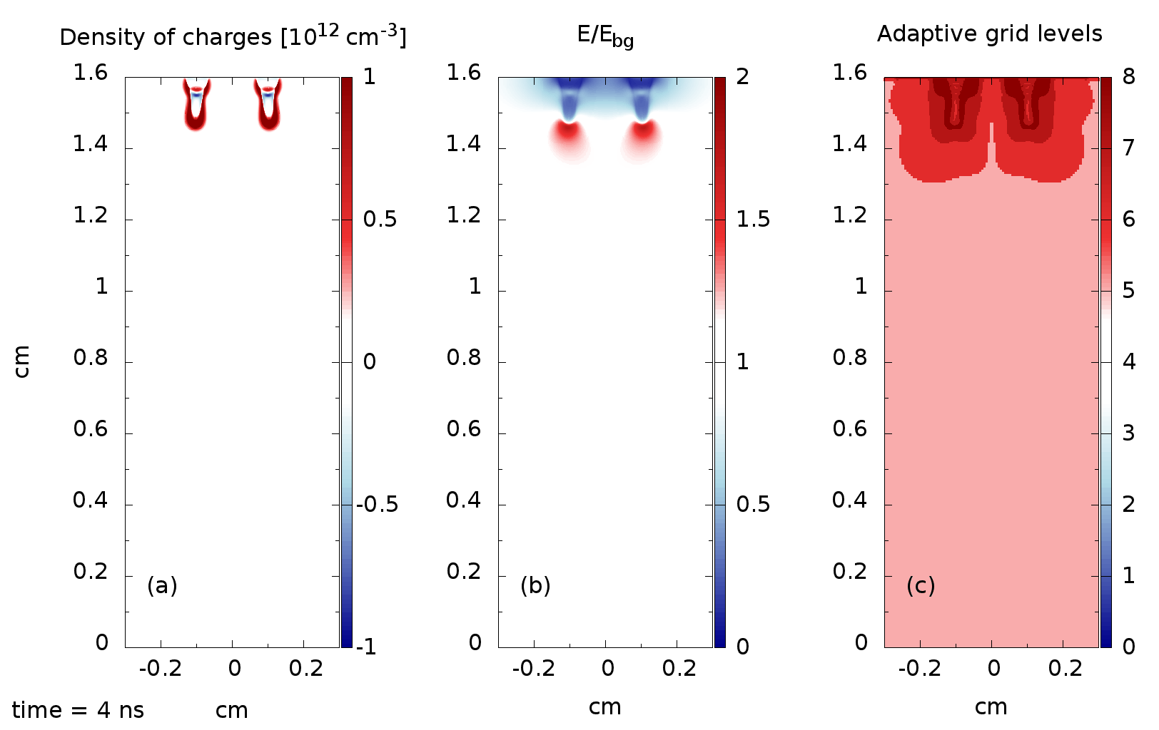
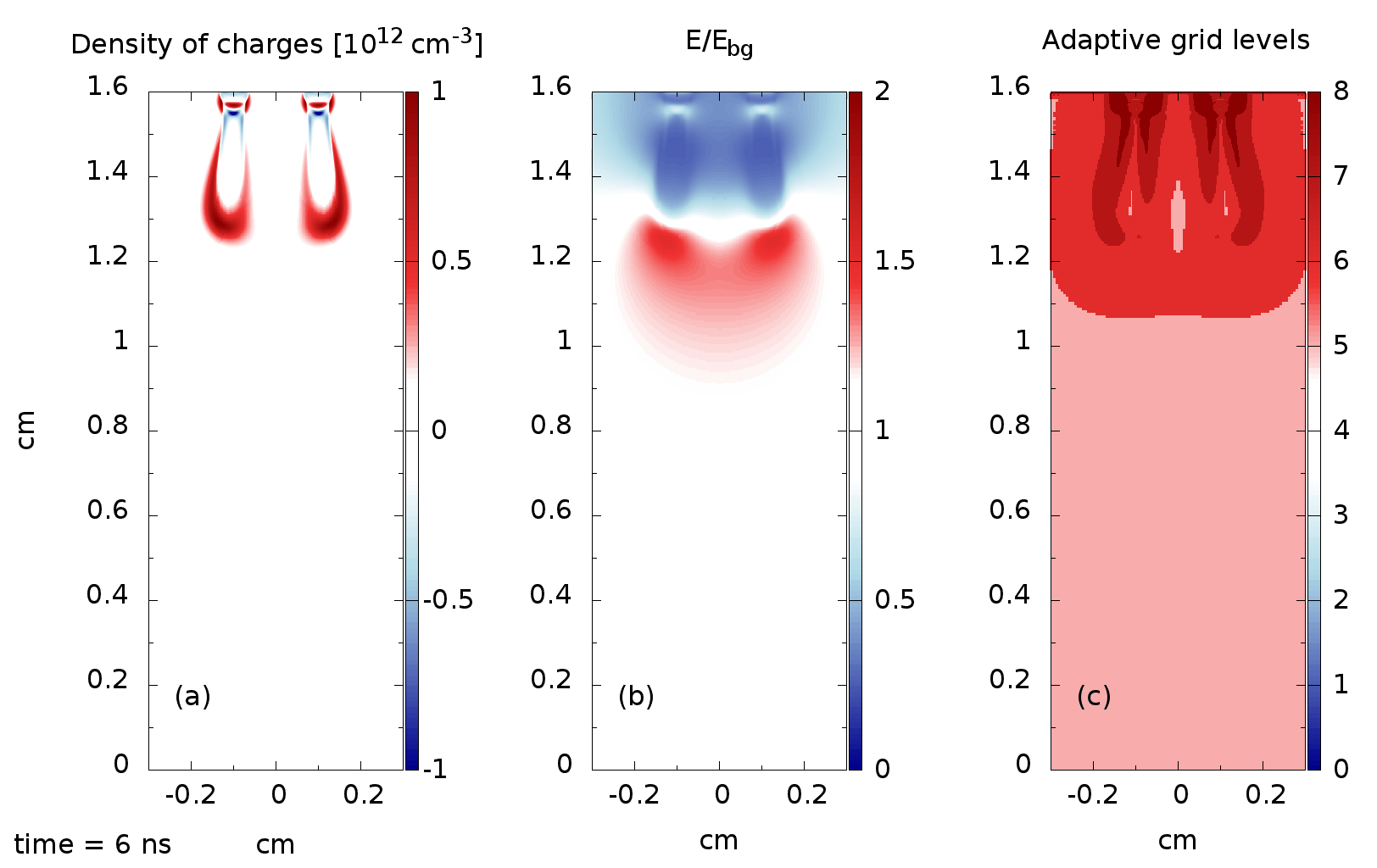
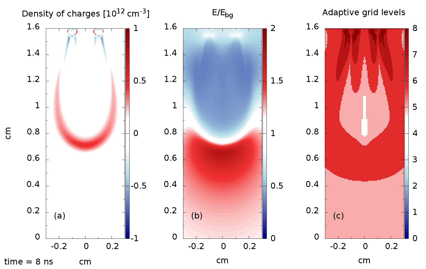
Let us consider two positive streamers modeled by (28)–(29) propagating in a homogeneous electric field. As before the system of equations is solved with the time-space adaptive scheme introduced in [26] with the Poisson equation discretized on the adapted grid following the numerical technique established in §3.2. The resulting linear systems are solved with MUMPS. The computational domain is given by $[0,3.0]\times[-1.6,1.6]\,$cm in a Cartesian configuration. A space-time accuracy tolerance of $\eta_{\rm MR}=\eta_{\mathcal{T}}=10^{-4}$ was chosen with a space resolution of 3.9$\,\mu$m corresponding to a finest grid-level of $J=8$ with $N_{{\rm R}x}=30$ and $N_{{\rm R}y}=32$. The finest spatial resolution is equivalent to that of a uniform grid with $8192\times 7680$ cells. A homogeneous electric field of ${\boldsymbol{E}}_{\rm bg}=(0,-48)\,$kV/cm is introduced via Dirichlet boundary conditions for the Poisson equation (29) at $y=\pm 1.6\,$cm, whilst Neumann boundary conditions are applied at $x=3.0\,$cm. A plane of symmetry is imposed at $x=0$. The positive streamer is initiated by placing a Gaussian seed with a maximum of $10^{13}\,$cm^-3 and a characteristic width of $0.02\,$cm, centered at $0.1\,$cm from the symmetry axis. The time evolution of the net charge density, the magnitude of the electric field, and the dynamic grid adaptation at time instances: $4.0$, $6.0$, and $8.0\,$ns are shown in Figure 8. Population of different grid-levels at sample times is detailed in Table 2 together with the corresponding data compression (DC), defined as the percentage of active cells with respect to the equivalent number of cells using the finest discretization, given in this case by 62914560. We recall that no grid overlapping is considered in this implementation, that is, both the time-dependent PDEs as well as the Poisson equations are solved on the adapted grid consisting of cells at different grid-levels as shown in Table 2. The coarsest resolution allowed in this simulation (at grid-level $j=1$) corresponds to a spatial resolution of $0.05\,$cm (note that this level was not populated during the simulation, therefore it is not listed in Table 2).

Table 2: Data compression (DC) and number of cells at different grid-levels at sample time instances.

time(ns)	DC(%)	Number of cells at grid-levels
		2	3	4	5	6	7	8
00	0.031	15240	162	272	527	1341	7728	169904
01	1.219	780	4671	61359	605154	22297	23160	49424
02	1.264	620	4440	57625	633483	23447	27668	47744
03	1.291	566	4346	56348	642443	26479	33016	48752
04	1.325	528	4528	54141	648333	34030	41660	50672
05	1.360	512	4712	51905	652364	42504	56536	47136
06	1.407	544	4768	49464	653958	61267	64120	51056
07	1.449	458	5288	47652	650502	93008	63196	51728
08	1.495	338	5791	46530	644986	131087	66656	45328
09	1.567	219	5388	48316	637538	188227	70380	35744
10	1.702	18	5296	48622	624126	294256	73264	25280

From Figure 8 and Table 2 we observe that the finest level is first populated at the vicinity of the initial Gaussian seed and follows the propagation of onsetting streamers (see Figure 8 corresponding to time $4\,$ns). At the next instance shown (Figure 8 at $6\,$ns), the propagating front is fully described in a region contained within levels 6 and 7. This is because both streamer heads had expanded and the finest scale is thus no longer necessary. Once the streamer heads have merged (Figure 8 at $8\,$ns) and therefore only one head is propagating, only level 6 is required. In particular behind the head, i.e., inside the plasma channel where neither sharp gradients nor strong discharge activity are present, the grid is coarsened down to level 4. The finest resolution is attained and kept throughout the simulation close to the initial Gaussian seeds where we can observe persistence of highly localized space charge as well as strong spatial variation of the electric field. Despite a decreasing population of the finest level after $7\,$ns (see Table 2) overall data compression is slowly increasing because discharge activity is gradually filling larger regions of the computational domain.

5 Concluding remarks

The multiresolution finite volume scheme [19] has been extended to include the numerical solution of Poisson equations on the corresponding adapted grids. A numerical procedure has been developed to represent the discrete Laplace operator on the adapted grid by reconstructing locally uniform-grid regions at inter-grid interfaces by means of ghost cells and inter-level multiresolution operations. This approach constitutes a new alternative to the standard level-wise numerical solution of elliptic equations considered in most of the adaptive mesh refinement techniques for time-dependent problems in the literature. The numerical solution of the discrete Poisson equation amounts to considering a linear system completely independent of the grid generation or any other grid-related data structure or geometric consideration. The multiresolution framework guarantees numerical approximations within an accuracy tolerance as well as consistency and conservation properties throughout the set of grids. Here we have focused our attention on Poisson equations, however the present technique remains valid for more general elliptic PDEs like Poisson equations with time- and/or space-varying coefficients.

The validity of the numerical strategy has been assessed in the context of the numerical simulation of streamer discharges. This application involves an intensive use of Poisson solvers and accurate solutions of Poisson equations are essential to the correct reproduction of physics. First, we have carefully evaluated the numerical errors introduced by data compression for a simpler configuration with analytical solution. A much more complex and complete model was then considered to simulate the propagation of a double-headed streamer discharge in air at atmospheric pressure. We have thus conducted a study on the performance and capabilities of various linear solvers for this problem. The latter allowed us to further validate the current implementation and serves as a guide for other applications. In particular we have evaluated the potentialities of algebraic multigrid solvers, well-suited for this kind of implementation with no geometric counterpart. The robustness of the numerical strategy has been further assessed for the simulation of interacting positive streamers, an interesting application in plasma physics.

Further developments include optimizing the numerical construction of the discrete Laplace operators by conceiving, for instance, better data structures or by updating only the matrix entries modified by grid adaptation. Taking into account that in this implementation solving the linear systems becomes a separate aspect from the multiresolution analysis itself, parallel computing capabilities may be directly inherited from the software packages available in the literature. However, an intelligent conjunction with multiresolution parallelism must be sought to achieve overall satisfactory results. These issues constitute particular topics of our current research.

Appendix A Multiresolution error estimate

Defining the pairs $(\phi_{j,k},\psi_{j,k})$ and $(\widetilde{\phi}_{j,k},\widetilde{\psi}_{j,k})$ as, respectively, the primal and the dual scaling function and wavelet, the following representations of $f_{j+1}$ are perfectly equivalent:

$$f_{j+1}:=\displaystyle\sum_{|\mu|=j+1}f_{\mu}\phi_{\mu}=\displaystyle\sum_{|\gamma|=j}f_{\gamma}\phi_{\gamma}+\displaystyle\sum_{|\gamma|=j}d_{\gamma}\psi_{\gamma},$$

with $f_{\mu}:=\langle f,\widetilde{\phi}_{\mu}\rangle$, $f_{\gamma}:=\langle f,\widetilde{\phi}_{\gamma}\rangle$, and $d_{\gamma}:=\langle f,\widetilde{\psi}_{\gamma}\rangle$. Iterating on $j$, we have the following wavelet decomposition,

$$f=\displaystyle\sum_{j=-1}^{\infty}\sum_{|\lambda|=j}\langle f,\widetilde{\psi}_{\lambda}\rangle\psi_{\lambda},$$

where $\psi_{-1,k}:=\phi_{0,k}$ and $\widetilde{\psi}_{-1,k}:=\widetilde{\phi}_{0,k}$. We can thus construct the array $\mathbf{\Psi}_{J,\lambda}$, $|\lambda|\leq J$, that corresponds to the primal wavelets $\psi_{\lambda}$ cell-averaged at level $J$, i.e., $\mathbf{\Psi}_{J,\lambda}:=(\langle\psi_{\lambda},\widetilde{\phi}_{\gamma}\rangle)_{\gamma\in S_{J}}$. For compactly supported wavelets, there is a constant $C>0$ such that

$$\|\mathbf{\Psi}_{J,\lambda}\|_{2}\leq C\|\psi_{\lambda}\|_{L^{2}}\leq C2^{-d|\lambda|/2},$$

and for the multiresolution approximation ${\mathcal{A}}_{\Lambda}\mathbf{f}_{J}$, we have that

$$\|\mathbf{f}_{J}-{\mathcal{A}}_{\Lambda}\mathbf{f}_{J}\|^{2}_{2}=\left\|d_{\lambda}\mathbf{\Psi}_{J,\lambda}|_{\lambda\notin\Lambda}\right\|^{2}_{2}\leq C\displaystyle\sum_{\lambda\notin\Lambda}\|d_{\lambda}\|_{L^{2}}^{2}2^{-d|\lambda|}=C\displaystyle\sum_{\|d_{\lambda}\|_{L^{2}}\leq\epsilon_{|\lambda|}}\|d_{\lambda}\|_{L^{2}}^{2}2^{-d|\lambda|},$$

because only some of the components of $(\mathbf{f}_{J}-{\mathcal{A}}_{\Lambda}\mathbf{f}_{J})$ are non-zero, namely those corresponding to discarded details; therefore, the approximation error is bounded by their sum. Considering a level-wise threshold parameter: $\epsilon_{j}:=2^{dj/2}\epsilon$, the next bound follows (where $\#(\cdot)$ returns the cardinality of a set):

$$\|\mathbf{f}_{J}-{\mathcal{A}}_{\Lambda}\mathbf{f}_{J}\|^{2}_{2}\leq C\#(\nabla^{J})\epsilon^{2}=C\#(S_{J})\epsilon^{2}\leq C2^{dJ}\epsilon^{2},$$

with the cautious assumption that $\|d_{\lambda}\|_{L^{2}}=\epsilon_{|\lambda|}$ for all $d_{\lambda}$ such that $\lambda\notin\Lambda$ (even though they might be much smaller than $\epsilon_{|\lambda|}$) as well as for the remaining components of $(\mathbf{f}_{J}-{\mathcal{A}}_{\Lambda}\mathbf{f}_{J})$ (even though they are zero). Choosing $\epsilon:=2^{-dJ/2}\eta_{\rm MR}$ then yields (12) with the level-dependent threshold values (13). Bound (12) is similarly shown in [19] for both a uniform and $\ell^{1}$ norms.

Appendix B Pseudo-code of the algorithm

We consider a multiresolution adapted grid given by the set of leaves: $\Theta_{\mathrm{L}}=(\Omega_{\lambda})_{h(\lambda)\in{\rm I}_{\mathrm{L}}}$, a one-dimensional array of size $N_{\rm L}$. The algorithm to construct the discrete Laplacian: $\mathbf{\widetilde{A}}\in{\mathcal{M}}_{n}({\mathbb{R}})$, can be schematically described as follows in a Cartesian finite volume framework where interfaces are given by $\Gamma^{d^{\prime}}_{\gamma,\mu}$, $d^{\prime}=1,\ldots,d$. This scheme supports polynomial interpolations (4) and finite volume space discretizations (21) of arbitrary order.

  Initialization: $\mathbf{\widetilde{A}}=0$.

  for $i=1\to N_{\rm L}$ do

     Current leaf: $\Omega_{\gamma}$ s.t. $\gamma=h^{-1}(i)$.

     for $d^{\prime}=1\to d$ do

        Current neighbor: $\Omega_{\mu}$ s.t. $\Gamma^{d^{\prime}}_{\gamma,\mu}=\overline{\Omega_{\gamma}}\cap\overline{\Omega_{\mu}}$.

        if $\mu\in D(h)$  then {$\Omega_{\mu}$ is a leaf, i.e., (i).}

           $i^{\prime}=h(\mu)$.

           for $\lambda\in R^{+}_{F}(\gamma)$ do

              if $\lambda\in D(h)$  then {$\Omega_{\lambda}$ is a leaf, i.e., (i).}

                 $l=h(\lambda)$.

                 $\widetilde{a}_{i,l}=\widetilde{a}_{i,l}+\alpha_{\gamma,\lambda}$.

                 $\widetilde{a}_{i^{\prime},l}=\widetilde{a}_{i^{\prime},l}-\alpha_{\gamma,\lambda}$.

              else if $\lambda\in\bigcup_{r=1}^{N_{\rm R}}{\mathrm{P}}(\Lambda_{r})$  then {$\Omega_{\lambda}$ is a phantom, i.e., (iii).}

                 for $\widehat{\lambda}$ s.t. $\widehat{\lambda}\in R_{I}(\lambda)$ do

                    if $\widehat{\lambda}\in D(h)$  then {$\Omega_{\widehat{\lambda}}$ is a leaf, i.e., (i).}

                       $l=h(\widehat{\lambda})$.

                       $\widetilde{a}_{i,l}=\widetilde{a}_{i,l}+\beta_{\lambda,\widehat{\lambda}}\alpha_{\gamma,\lambda}$.

                       $\widetilde{a}_{i^{\prime},l}=\widetilde{a}_{i^{\prime},l}-\beta_{\lambda,\widehat{\lambda}}\alpha_{\gamma,\lambda}$.

                    else {$\Omega_{\widehat{\lambda}}$ is within the tree, i.e., (ii).}

                       for $\widehat{\lambda}^{\prime}$ s.t. $\Omega_{\widehat{\lambda}^{\prime}}\subset\Omega_{\widehat{\lambda}}$ do

                          if $\widehat{\lambda}^{\prime}\in D(h)$  then {$\Omega_{\widehat{\lambda}^{\prime}}$ is a leaf, i.e., (i).}

                             $l=h(\widehat{\lambda}^{\prime})$.

                             $\widetilde{a}_{i,l}=\widetilde{a}_{i,l}+|\Omega_{\widehat{\lambda}}|^{-1}|\Omega_{\widehat{\lambda}^{\prime}}|\beta_{\lambda,\widehat{\lambda}}\alpha_{\gamma,\lambda}$.

                             $\widetilde{a}_{i^{\prime},l}=\widetilde{a}_{i^{\prime},l}-|\Omega_{\widehat{\lambda}}|^{-1}|\Omega_{\widehat{\lambda}^{\prime}}|\beta_{\lambda,\widehat{\lambda}}\alpha_{\gamma,\lambda}$.

                          else

                             for $\widehat{\lambda}^{\prime\prime}$ s.t. $\Omega_{\widehat{\lambda}^{\prime\prime}}\subset\Omega_{\widehat{\lambda}^{\prime}}$ do

                                if $\widehat{\lambda}^{\prime\prime}\in D(h)$  then {$\Omega_{\widehat{\lambda}^{\prime\prime}}$ is a leaf, i.e., (i).}

                                   $l=h(\widehat{\lambda}^{\prime\prime})$.

                                   $\widetilde{a}_{i,l}=\widetilde{a}_{i,l}+|\Omega_{\widehat{\lambda}}|^{-1}|\Omega_{\widehat{\lambda}^{\prime\prime}}|\beta_{\lambda,\widehat{\lambda}}\alpha_{\gamma,\lambda}$.

                                   $\widetilde{a}_{i^{\prime},l}=\widetilde{a}_{i^{\prime},l}-|\Omega_{\widehat{\lambda}}|^{-1}|\Omega_{\widehat{\lambda}^{\prime\prime}}|\beta_{\lambda,\widehat{\lambda}}\alpha_{\gamma,\lambda}$.

                                else

                                   Continue up to leaves.

                                end if

                             end for

                          end if

                       end for

                    end if

                 end for

              else {$\Omega_{\lambda}$ is within the tree, i.e., (ii).}

                 for $\lambda^{\prime}$ s.t. $\Omega_{\lambda^{\prime}}\subset\Omega_{\lambda}$ do

                    if $\lambda^{\prime}\in D(h)$  then {$\Omega_{\lambda^{\prime}}$ is a leaf, i.e., (i).}

                       $l=h(\lambda^{\prime})$.

                       $\widetilde{a}_{i,l}=\widetilde{a}_{i,l}+|\Omega_{\lambda}|^{-1}|\Omega_{\lambda^{\prime}}|\alpha_{\gamma,\lambda}$.

                       $\widetilde{a}_{i^{\prime},l}=\widetilde{a}_{i^{\prime},l}-|\Omega_{\lambda}|^{-1}|\Omega_{\lambda^{\prime}}|\alpha_{\gamma,\lambda}$.

                    else

                       Continue up to leaves.

                    end if

                 end for

              end if

           end for

        else if $\mu\in\bigcup_{r=1}^{N_{\rm R}}{\mathrm{P}}(\Lambda_{r})$  then {$\Omega_{\mu}$ is a phantom, i.e., (iii).}

           for $\lambda\in R^{+}_{F}(\gamma)$ do

              if $\lambda\in D(h)$  then {$\Omega_{\lambda}$ is a leaf, i.e., (i).}

                 $l=h(\lambda)$.

                 $\widetilde{a}_{i,l}=\widetilde{a}_{i,l}+\alpha_{\gamma,\lambda}$.

                 for $\widehat{\mu}$ s.t. $\Omega_{\mu}\subset\Omega_{\widehat{\mu}}\wedge\overline{\Omega_{\gamma}}\cap\overline{\Omega_{\widehat{\mu}}}\neq\varnothing$ do

                    $i^{\prime}=h(\widehat{\mu})$.

                    $\widetilde{a}_{i^{\prime},l}=\widetilde{a}_{i^{\prime},l}-|\Omega_{\widehat{\mu}}|^{-1}|\Omega_{\mu}|\alpha_{\gamma,\lambda}$.

                 end for

              else if $\lambda\in\bigcup_{r=1}^{N_{\rm R}}{\mathrm{P}}(\Lambda_{r})$  then {$\Omega_{\lambda}$ is a phantom, i.e., (iii).}

                 for $\widehat{\lambda}$ s.t. $\widehat{\lambda}\in R_{I}(\lambda)$ do

                    if $\widehat{\lambda}\in D(h)$  then {$\Omega_{\widehat{\lambda}}$ is a leaf, i.e., (i).}

                       $l=h(\widehat{\lambda})$.

                       $\widetilde{a}_{i,l}=\widetilde{a}_{i,l}+\beta_{\lambda,\widehat{\lambda}}\alpha_{\gamma,\lambda}$.

                       for $\widehat{\mu}$ s.t. $\Omega_{\mu}\subset\Omega_{\widehat{\mu}}\wedge\overline{\Omega_{\gamma}}\cap\overline{\Omega_{\widehat{\mu}}}\neq\varnothing$ do

                          $i^{\prime}=h(\widehat{\mu})$.

                          $\widetilde{a}_{i^{\prime},l}=\widetilde{a}_{i^{\prime},l}-|\Omega_{\widehat{\mu}}|^{-1}|\Omega_{\mu}|\beta_{\lambda,\widehat{\lambda}}\alpha_{\gamma,\lambda}$.

                       end for

                    else {$\Omega_{\widehat{\lambda}}$ is within the tree, i.e., (ii).}

                       Continue up to leaves.

                    end if

                 end for

              else {$\Omega_{\lambda}$ is within the tree, i.e., (ii).}

                 Continue up to leaves.

              end if

           end for

        else {$\Omega_{\mu}$ is within the tree, i.e., (ii).}

           for $\widehat{\gamma}$ s.t. $\Omega_{\widehat{\gamma}}\subset\Omega_{\gamma}\wedge\overline{\Omega_{\widehat{\gamma}}}\cap\overline{\Omega_{\mu}}\neq\varnothing$ do

              Current neighbor: $\Omega_{\mu^{\prime}}$ s.t. $\Omega_{\mu^{\prime}}\subset\Omega_{\mu}\wedge\Gamma^{d^{\prime}}_{\widehat{\gamma},\mu^{\prime}}=\overline{\Omega_{\widehat{\gamma}}}\cap\overline{\Omega_{\mu^{\prime}}}$.

              $\Omega_{\mu^{\prime}}$ is a leaf: $i^{\prime}=h(\mu^{\prime})$.

              for $\lambda\in R^{+}_{F}(\widehat{\gamma})$ do

                 if $\lambda\in D(h)$  then {$\Omega_{\lambda}$ is a leaf, i.e., (i).}

                    $l=h(\lambda)$.

                    $\widetilde{a}_{i,l}=\widetilde{a}_{i,l}+|\Omega_{\gamma}|^{-1}|\Omega_{\widehat{\gamma}}|\alpha_{\widehat{\gamma},\lambda}$.

                    $\widetilde{a}_{i^{\prime},l}=\widetilde{a}_{i^{\prime},l}-\alpha_{\widehat{\gamma},\lambda}$.

                 else if $\lambda\in\bigcup_{r=1}^{N_{\rm R}}{\mathrm{P}}(\Lambda_{r})$  then {$\Omega_{\lambda}$ is a phantom, i.e., (iii).}

                    for $\widehat{\lambda}$ s.t. $\widehat{\lambda}\in R_{I}(\lambda)$ do

                       if $\widehat{\lambda}\in D(h)$  then {$\Omega_{\widehat{\lambda}}$ is a leaf, i.e., (i).}

                          $l=h(\widehat{\lambda})$.

                          $\widetilde{a}_{i,l}=\widetilde{a}_{i,l}+|\Omega_{\gamma}|^{-1}|\Omega_{\widehat{\gamma}}|\beta_{\lambda,\widehat{\lambda}}\alpha_{\widehat{\gamma},\lambda}$.

                          $\widetilde{a}_{i^{\prime},l}=\widetilde{a}_{i^{\prime},l}-\beta_{\lambda,\widehat{\lambda}}\alpha_{\widehat{\gamma},\lambda}$.

                       else {$\Omega_{\widehat{\lambda}}$ is within the tree, i.e., (ii).}

                          Continue up to leaves.

                       end if

                    end for

                 else {$\Omega_{\lambda}$ is within the tree, i.e., (ii).}

                    Continue up to leaves.

                 end if

              end for

           end for

        end if

     end for

  end for

Appendix C Photoionization model

The photoionization source term $S_{\rm ph}$ is evaluated using the three-group SP₃ model developed in [11] with Larsen’s boundary conditions [38, 39]. This model considers $N_{g}=3$ effective monochromatic radiative transfer equations. As no scattering of photons is taken into account and since the time scale of photon propagation is considered short with respect to the streamer propagation, at each instant of the streamer simulation the photon distribution function $\Psi_{\!l}({\boldsymbol{x}},{\boldsymbol{\Omega}})$ at position ${\boldsymbol{x}}$ and direction ${\boldsymbol{\Omega}}$ fulfills a radiative transfer equation of the form:

$${{\boldsymbol{\Omega}}}\cdot\partial_{\boldsymbol{x}}\Psi_{\!l}({\boldsymbol{x}},{\boldsymbol{\Omega}})+\lambda_{l}p_{{\rm O}_{2}}\Psi_{\!l}({\boldsymbol{x}},{\boldsymbol{\Omega}})=\frac{1}{4\pi}\frac{p_{\rm q}}{p+p_{\rm q}}\left(\xi\frac{\nu_{\rm u}}{\nu_{\rm i}}\right)\frac{\nu_{\rm i}n_{\rm e}}{c\,\xi},\quad l=1,\dots,N_{g},$$ (33)

where $l$ indicates discrete wavelengths, $\lambda_{l}$ is the absorption coefficient, $p_{{\rm O}_{2}}$ is the partial pressure of molecular oxygen ($150\,$Torr at atmospheric pressure), $p$ is the total pressure, $p_{\rm q}=30\,$Torr is the quenching pressure, $\xi=0.1$ is the photoionization efficiency, $\nu_{\rm u}$ is the effective excitation coefficient for N₂ states responsible for ionizing radiation, and $\nu_{\rm i}$ and $n_{\rm e}$ are, respectively, the previously introduced ionization coefficient and electron density. The term $(\xi\nu_{\rm u}/\nu_{\rm i})$ is given as a function of the reduced electric field in [62, 40]. Finally, $c$ stands for the speed of light. Let us emphasize that monochromatic equations (33) have different absorption coefficients but they all have the same source term that depends on the local reduced electric field $E/N_{\rm air}$, varying therefore in time and space.

The SP₃ approximation of (33) leads to a set of two elliptic equations for functions $\phi_{1,l}({\boldsymbol{x}})$ and $\phi_{2,l}({\boldsymbol{x}})$ [38]:

$$\left.\begin{array}[]{l}\displaystyle\partial_{\boldsymbol{x}}^{2}\phi_{1,l}({\boldsymbol{x}})-\frac{\lambda_{l}^{2}p_{\rm O_{2}}^{2}}{\kappa_{1}^{2}}\phi_{1,l}({\boldsymbol{x}})=-\frac{\lambda_{l}p_{\rm O_{2}}}{\kappa_{1}^{2}}\frac{p_{\rm q}}{p+p_{\rm q}}\left(\xi\frac{\nu_{\rm u}}{\nu_{\rm i}}\right)\frac{\nu_{\rm i}n_{\rm e}}{c\,\xi},\\[6.45831pt] \displaystyle\partial_{\boldsymbol{x}}^{2}\phi_{2,l}({\boldsymbol{x}})-\frac{\lambda_{l}^{2}p_{\rm O_{2}}^{2}}{\kappa_{2}^{2}}\phi_{2,l}({\boldsymbol{x}})=-\frac{\lambda_{l}p_{\rm O_{2}}}{\kappa_{2}^{2}}\frac{p_{\rm q}}{p+p_{\rm q}}\left(\xi\frac{\nu_{\rm u}}{\nu_{\rm i}}\right)\frac{\nu_{\rm i}n_{\rm e}}{c\,\xi},\end{array}\right\}$$ (34)

with $\kappa_{1,2}=(1/7)(3\pm 2\sqrt{6/5})$. Equations (34) are coupled through the boundary condition. On a boundary surface with neither reflection nor emission, functions $\phi_{1,l}({\boldsymbol{x}})$ and $\phi_{2,l}({\boldsymbol{x}})$ must verify the following conditions [38, 39]:

$$\left.\begin{array}[]{l}\partial_{\boldsymbol{x}}\phi_{1,l}({\boldsymbol{x}})\cdot{\boldsymbol{n}}_{s}=-\lambda_{l}p_{\rm O_{2}}\alpha_{1}\phi_{1,l}({\boldsymbol{x}})-\lambda_{l}p_{\rm O_{2}}\beta_{2}\phi_{2,l}({\boldsymbol{x}}),\\[6.45831pt] \partial_{\boldsymbol{x}}\phi_{2,l}({\boldsymbol{x}})\cdot{\boldsymbol{n}}_{s}=-\lambda_{l}p_{\rm O_{2}}\alpha_{2}\phi_{2,l}({\boldsymbol{x}})-\lambda_{l}p_{\rm O_{2}}\beta_{1}\phi_{1,l}({\boldsymbol{x}}),\end{array}\right\}$$ (35)

where ${\boldsymbol{n}}_{s}$ is the outward unit normal to the boundary surface, $\alpha_{1,2}=(5/96)(34\pm 11\sqrt{6/5})$, and $\beta_{1,2}=(5/96)(2\pm\sqrt{6/5})$. Because $0<\beta_{1,2}\ll\alpha_{1,2}$ the coupling in (34) is weak. A simple strategy to solve (34) together with the boundary conditions (35) consist in solving the equations independently, that is, with $\beta_{1,2}=0$ to then iterate and correct the initial approximations with the inclusion of the $\beta_{1,2}$ coefficients. Convergence is attained very rapidly after few iterations (typically three). The isotropic part of the photon distribution function $\Psi_{\!l}({\boldsymbol{x}})$ is then written as a linear combination of $\phi_{1,l}({\boldsymbol{x}})$ and $\phi_{2,l}({\boldsymbol{x}})$ [38]:

$$\Psi_{\!l}({\boldsymbol{x}})=\frac{\gamma_{2}\phi_{1,l}({\boldsymbol{x}})-\gamma_{1}\phi_{2,l}({\boldsymbol{x}})}{\gamma_{2}-\gamma_{1}},$$

with $\gamma_{1,2}=(5/7)(1\pm 3\sqrt{5/6})$. The photoionization source term $S_{\rm ph}({\boldsymbol{x}})$ can be finally calculated as [11]:

$$S_{\rm ph}({\boldsymbol{x}})=\sum\limits_{l=1}^{N_{g}}A_{l}\xi p_{\rm O_{2}}c\Psi_{\!l}({\boldsymbol{x}}),$$

where parameters $A_{l}$ together with $\lambda_{l}$ are given in Table 3.

Table 3: Parameters for three group photoionization model [11].

$l$	$A_{l}\,[{\rm cm}^{-1}\,{\rm Torr}^{-1}]$	$\lambda_{l}[{\rm cm}^{-1}\,{\rm Torr}^{-1}]$
1	0.0067	0.0447
2	0.0346	0.1121
3	0.3059	0.5994

References

- [1] A.S. Almgren, J.B. Bell, P. Colella, L.H. Howell, and M.L. Welcome. A conservative adaptive projection method for the variable density incompressible Navier-Stokes equations. J. Comput. Phys., 142(1):1–46, 1998.
- [2] P.R. Amestoy, I.S. Duff, J. Koster, and J.-Y. L’Excellent. A fully asynchronous multifrontal solver using distributed dynamic scheduling. SIAM J. Matrix Anal. Appl., 23(1):15–41, 2001.
- [3] P.R. Amestoy, I.S. Duff, and J.-Y. L’Excellent. Multifrontal parallel distributed symmetric and unsymmetric solvers. Comput. Methods in Appl. Mech. Eng., 184(2-4):501–520, 2000.
- [4] N.Y Babaeva and G.V. Naidis. Two-dimensional modelling of positive streamer dynamics in non-uniform electric fields in air. J. Phys. D-Appl. Phys., 29:2423–2431, 1996.
- [5] A. Barinka, T. Barsch, P. Charton, A. Cohen, S. Dahlke, W. Dahmen, and K. Urban. Adaptive wavelet schemes for elliptic problems–implementation and numerical experiments. SIAM J. Sci. Comput., 23(3):910–939, 2001.
- [6] M.S. Benilov and G.V. Naidis. Modelling of low-current discharges in atmospheric-pressure air taking account of non-equilibrium effects. J. Phys. D-Appl. Phys., 36(15):1834–1841, 2003.
- [7] M.J. Berger and P. Colella. Local adaptive mesh refinement for shock hydrodynamics. J. Comput. Phys., 82:67–84, 1989.
- [8] M.J. Berger and J. Oliger. Adaptive mesh refinement for hyperbolic partial differential equations. J. Comput. Phys., 53:484–512, 1984.
- [9] B.L. Bihari and A. Harten. Multiresolution schemes for the numerical solution of 2-D conservation laws I. SIAM J. Sci. Comput., 18(2):315–354, 1997.
- [10] Z. Bonaventura, M. Duarte, A. Bourdon, and M. Massot. Derivation of a merging condition for two interacting streamers in air. Plasma Sources Sci. Technol., 21(5):052001, 2012.
- [11] A. Bourdon, V.P. Pasko, N.Y. Liu, S. Celestin, P. Ségur, and E. Marode. Efficient models for photoionization produced by non-thermal gas discharges in air based on radiative transfer and the Helmholtz equations. Plasma Sources Sci. Technol., 16(3):656–678, 2007.
- [12] T.M.P. Briels, J. Kos, E.M. van Veldhuizen, and U. Ebert. Circuit dependence of the diameter of pulsed positive streamers in air. J. Phys. D-Appl. Phys., 39(24):5201–5210, 2006.
- [13] K. Brix, S. Melian, S. Müller, and M. Bachmann. Adaptive multiresolution methods: Practical issues on data structures, implementation and parallelization. ESAIM: Proc., 34:151–183, 2011.
- [14] R. Bürger, R. Ruiz-Baier, K. Schneider, and M. Sepúlveda. Fully adaptive multiresolution schemes for strongly degenerate parabolic equations in one space dimension. ESAIM: Math. Model. Numer. Anal., 42:535–563, 2008.
- [15] A.J. Chorin. Numerical solution of the Navier-Stokes equations. Math. Comp., 22:745–762, 1968.
- [16] A. Cohen. Wavelet Methods in Numerical Analysis, volume 7. Elsevier, Amsterdam, 2000.
- [17] A. Cohen, W. Dahmen, and R. DeVore. Adaptive wavelet methods for elliptic operator equations: Convergence rates. Math. Comp., 70:27–75, 2001.
- [18] A. Cohen, I. Daubechies, and J.-C. Feauveau. Biorthogonal bases of compactly supported wavelets. Comm. Pure Appl. Math., 45(5):485–560, 1992.
- [19] A. Cohen, S.M. Kaber, S. Müller, and M. Postel. Fully adaptive multiresolution finite volume schemes for conservation laws. Math. Comp., 72:183–225, 2003.
- [20] A. Cohen and R. Masson. Wavelet methods for second-order elliptic problems, preconditioning, and adaptivity. SIAM J. Sci. Comput., 21(3):1006–1026, 1999.
- [21] A. Cohen and R. Masson. Wavelet adaptive method for second order elliptic problems: boundary conditions and domain decomposition. Numer. Math., 86(2):193–238, 2000.
- [22] S.A. Cummer, N. Jaugey, J.B. Li, W.A. Lyons, T.E. Nelson, and E.A. Gerken. Submillisecond imaging of sprite development and structure. Geophys. Res. Lett., 33(4):L04104, 2006.
- [23] S. Dahlke, W. Dahmen, and R.A. DeVore. Nonlinear approximation and adaptive techniques for solving elliptic operator equations. In W. Dahmen, A.J. Kurdila, and P. Oswald, editors, Multiscale Wavelet Methods for Partial Differential Equations, volume 6 of Wavelet Analysis and Its Applications, pages 237–283. Academic Press, 1997.
- [24] M. Domingues, S. Gomes, O. Roussel, and K. Schneider. Adaptive multiresolution methods. ESAIM: Proc., 34:1–96, 2011.
- [25] M. Duarte. Méthodes numériques adaptatives pour la simulation de la dynamique de fronts de réaction multi-échelles en temps et en espace. PhD thesis, Ecole Centrale Paris, France, 2011.
- [26] M. Duarte, Z. Bonaventura, M. Massot, A. Bourdon, S. Descombes, and T. Dumont. A new numerical strategy with space-time adaptivity and error control for multi-scale streamer discharge simulations. J. Comput. Phys., 231:1002–1019, 2012.
- [27] M. Duarte, S. Descombes, C. Tenaud, S. Candel, and M. Massot. Time-space adaptive numerical methods for the simulation of combustion fronts. Combust. Flame, (160):1083–1101, 2013.
- [28] M. Duarte, M. Massot, S. Descombes, C. Tenaud, T. Dumont, V. Louvet, and F. Laurent. New resolution strategy for multi-scale reaction waves using time operator splitting, space adaptive multiresolution and dedicated high order implicit/explicit time integrators. SIAM J. Sci. Comput., 34(1):A76–A104, 2012.
- [29] T. Dumont, M. Duarte, S. Descombes, M.-A. Dronne, M. Massot, and V. Louvet. Simulation of human ischemic stroke in realistic 3D geometry. Commun. Nonlinear Sci. Numer. Simul., 18(6):1539–1557, 2013.
- [30] U. Ebert, F. Brau, G. Derks, W. Hundsdorfer, C.-Y. Kao, C. Li, A. Luque, B. Meulenbroek, S. Nijdam, V. Ratushnaya, L. Schäfer, and S. Tanveer. Multiple scales in streamer discharges, with an emphasis on moving boundary approximations. Nonlinearity, 24(1):C1–C26, 2011.
- [31] J.L. Guermond, P. Minev, and J. Shen. An overview of projection methods for incompressible flows. Comput. Method Appl. Mech. Eng., 195(44–47):6011–6045, 2006.
- [32] A. Harten. Adaptive multiresolution schemes for shock computations. J. Comput. Phys., 115:319–338, 1994.
- [33] A. Harten. Multiresolution algorithms for the numerical solution of hyperbolic conservation laws. Comm. Pure Appl. Math., 48:1305–1342, 1995.
- [34] V.E. Henson and U.M. Yang. BoomerAMG: A parallel algebraic multigrid solver and preconditioner. Appl. Numer. Math., 41:155–177, 2002.
- [35] S. Jaffard. Wavelet methods for fast resolution of elliptic problems. SIAM J. Numer. Anal., 29(4):965–986, 1992.
- [36] I.A. Kossyi, A.Y. Kostinsky, A.A. Matveyev, and V.P. Silakov. Kinetic scheme of the non-equilibrium discharge in nitrogen-oxygen mixtures. Plasma Sources Sci. Technol., 1(3):207–220, 1992.
- [37] A.A. Kulikovsky. Positive streamer between parallel plate electrodes in atmospheric pressure air. J. Phys. D-Appl. Phys., 30:441–450, 1997.
- [38] E.W. Larsen, G. Thommes, A. Klar, M. Seaid, and T. Gotz. Simplified P-N approximations to the equations of radiative heat transfer and applications. J. Comput. Phys., 183(2):652–675, 2002.
- [39] N.Y. Liu, S. Celestin, A. Bourdon, V.P. Pasko, P. Ségur, and E. Marode. Application of photoionization models based on radiative transfer and the Helmholtz equations to studies of streamers in weak electric fields. Appl. Phys. Lett., 91(21):211501, 2007.
- [40] N.Y. Liu and V.P. Pasko. Effects of photoionization on propagation and branching of positive and negative streamers in sprites. J. Geophys. Res., 109:A04301, 2004.
- [41] A. Luque, U. Ebert, and W. Hundsdorfer. Interaction of streamer discharges in air and other oxygen-nitrogen mixtures. Phys. Rev. Lett., 101(7):075005, 2008.
- [42] D.F. Martin, P. Colella, and D. Graves. A cell-centered adaptive projection method for the incompressible Navier-Stokes equations in three dimensions . J. Comput. Phys., 227(3):1863–1886, 2008.
- [43] C. Montijn, W. Hundsdorfer, and U. Ebert. An adaptive grid refinement strategy for the simulation of negative streamers. J. Comput. Phys., 219(2):801–835, 2006.
- [44] R. Morrow and J.J. Lowke. Streamer propagation in air. J. Phys. D-Appl. Phys., 30:614–627, 1997.
- [45] S. Müller. Adaptive Multiscale Schemes for Conservation Laws, volume 27. Springer-Verlag, 2003.
- [46] S. Müller. Multiresolution schemes for conservation laws. In R. DeVore et al., editor, Multiscale, Nonlinear and Adaptive Approximation, pages 379–408. Springer Berlin Heidelberg, 2009.
- [47] A. Napov and Y. Notay. An algebraic multigrid method with guaranteed convergence rate. SIAM J. Sci. Comput., 34:A1079–A1109, 2012.
- [48] S. Nijdam, C.G.C. Geurts, E.M. van Veldhuizen, and U. Ebert. Reconnection and merging of positive streamers in air. J. Phys. D-Appl. Phys., 42(4):045201, 2009.
- [49] Y. Notay. An aggregation-based algebraic multigrid method. Electronic Trans. Numer. Anal., 37:123–146, 2010.
- [50] Y. Notay. Aggregation-based algebraic multigrid for convection-diffusion equations. SIAM J. Sci. Comput., 34:A2288–A2316, 2012.
- [51] S. Pancheshnyi, P. Ségur, J. Capeillère, and A. Bourdon. Numerical simulation of filamentary discharges with parallel adaptive mesh refinement. J. Comp. Phys., 227(13):6574–6590, 2008.
- [52] O. Roussel, K. Schneider, A. Tsigulin, and H. Bockhorn. A conservative fully adaptive multiresolution algorithm for parabolic PDEs. J. Comput. Phys., 188(2):493–523, 2003.
- [53] Y. Saad and M. Schultz. GMRES: A Generalized Minimal Residual Algorithm for Solving Nonsymmetric Linear Systems. SIAM J. Sci. Stat. Comp., 7(3):856–869, 1986.
- [54] C. Safta, J. Ray, and H.N. Najm. A high-order low-Mach number AMR construction for chemically reacting flows. J. Comput. Phys., 229(24):9299–9322, 2010.
- [55] K. Schneider and O.V. Vasilyev. Wavelet methods in computational fluid dynamics. Annu. Rev. Fluid Mech., 42:473–503, 2010.
- [56] R. Témam. Sur l’approximation de la solution des équations de Navier-Stokes par la méthode des pas fractionnaires. II. Arch. Rational Mech. Anal., 33:377–385, 1969.
- [57] R. Teyssier. Cosmological hydrodynamics with adaptive mesh refinement - A new high resolution code called RAMSES. A&A, 385(1):337–364, 2002.
- [58] T. Unfer, J.-P. Boeuf, F. Rogier, and F. Thivet. Multi-scale gas discharge simulations using asynchronous adaptive mesh refinement. Comput. Phys. Commun., 181(2):247–258, 2010.
- [59] O.V. Vasilyev. Solving multi-dimensional evolution problems with localized structures using second generation wavelets. Int. J. Comp. Fluid Dyn., 17:151–168, 2003.
- [60] O.V. Vasilyev and C. Bowman. Second-generation wavelet collocation method for the solution of partial differential equations. J. Comput. Phys., 165(2):660–693, 2000.
- [61] O.V. Vasilyev and N.K.-R. Kevlahan. An adaptive multilevel wavelet collocation method for elliptic problems. J. Comput. Phys., 206(2):412–431, 2005.
- [62] M.B. Zheleznyak, A.K. Mnatsakanyan, and S.V. Sizykh. Photo ionization of nitrogen and oxygen mixtures by radiation from a gas discharge. High Temp., 20(3):357–362, 1982.