A Hybrid MPI-OpenMP parallel implementation for pseudospectral simulations with application to Taylor–Couette Flow

Abstract

A hybrid-parallel direct-numerical-simulation method with application to turbulent Taylor–Couette flow is presented. The Navier–Stokes equations are discretized in cylindrical coordinates with the spectral Fourier–Galerkin method in the axial and azimuthal directions, and high-order finite differences in the radial direction. Time is advanced by a second-order, semi-implicit projection scheme, which requires the solution of five Helmholtz/Poisson equations, avoids staggered grids and renders very small slip velocities. Nonlinear terms are evaluated with the pseudospectral method. The code is parallelized using a hybrid MPI-OpenMP strategy, which, compared with a flat MPI parallelization, is simpler to implement, allows to reduce inter-node communications and MPI overhead that become relevant at high processor-core counts, and helps to contain the memory footprint. A strong scaling study shows that the hybrid code maintains scalability up to more than 20 000 processor cores and thus allows to perform simulations at higher resolutions than previously feasible. In particular, it opens up the possibility to simulate turbulent Taylor-Couette flows at Reynolds numbers up to $\mathcal{O}(10^{5})$. This enables to probe hydrodynamic turbulence in Keplerian flows in experimentally relevant regimes.

1 Introduction

Rotating fluid flows with radially increasing angular momentum are known to be linearly stable because of the inviscid Rayleigh criterion [1]. A particularly important application is astrophysical Keplerian flow, with angular velocity profile decreasing radially as $\Omega\propto r^{-3/2}$. Whether Keplerian flows become turbulent because of nonlinear instabilities or remain laminar even at extreme Reynolds numbers, has great implications for accretion processes in weakly-ionized astrophysical disks [2]. This question has been recently investigated with experiments of fluid flows between rotating cylinders (Taylor–Couette flow, TCf), which can in principle approximate Keplerian profiles. Experiments conducted by Ji and co-workers [3, 4, 5] found no hydrodynamic turbulence in quasi-Keplerian TCf in the range $Re\sim\mathcal{O}(10^{5}-10^{6})$, whereas similar studies [6, 7] report strongly turbulent flows that could account for the observed accretion rates in astrophysical disks. This discrepancy may arise from the axial boundary conditions: numerical simulations of the experimental setups show that top and bottom endwalls confining the fluid strongly disrupt Keplerian velocity profiles and causes turbulence to arise already at $Re\sim\mathcal{O}(10^{3})$ [8]. Hence, the interpretation and extrapolation of experimental data remains controversial because of the prominent role played by axial endwalls.

Numerical simulations with axially periodic boundaries resolve this problem and allow to directly probe the stability of Keplerian flows. Very recently, Ostilla-Mónico et al. [9] have carried out such simulations at $Re=8.1\times 10^{4}$ and observed that the turbulence decays to laminar flow. However, the role of initial conditions and numerical dissipation in the decay process are unknown and require more detailed studies. Probing the stability of Keplerian flows requires achieving yet larger Reynolds numbers $Re\sim\mathcal{O}(10^{5})$, while still resolving the dissipation scales. We note that as the key question is concerned about the existence of turbulence, modeling strategies such as Reynolds-averaged equations (RANS) and Large-Eddy Simulation (LES) are precluded and one has to resort to direct numerical simulation (DNS) of the Navier–Stokes equations (see [10] for details about these simulation techniques). Starting with the study of homogeneous isotropic turbulence conducted by Orszag and Patterson [11], DNS has been proven as a very powerful approach to explore the physics of turbulent flows (see Ref. [12, 13]). It has been widely used in fundamental research on both transitional and fully-developed turbulence in boundary layers over a flat plate (e.g. [14, 15]), channel (e.g. [16, 17]), pipe (e.g. [18, 19]) and Taylor–Couette flows (e.g. [20, 21, 22]). Distinguished from RANS and LES, a carefully performed DNS resolves all temporal and spatial scales relevant to turbulence and thus provides data of high fidelity. Its advantage is also its main drawback: resolving the physics of turbulence implies a scaling of the computational complexity as $\mathcal{O}(Re^{3})$ [10].

In this paper we develop a highly efficient DNS code for TCf with axially periodic boundary conditions using a hybrid two-level parallelization strategy. It enables DNS to be performed up to $Re\sim\mathcal{O}(10^{5})$, and thus provides access to a broad range in the parameter space of TCf, including quasi-Keplerian flows at experimentally relevant Reynolds numbers. Generally, finite differences [9] or spectral-element methods [21] can be used to perform DNS of Taylor–Couette flow at large Reynolds numbers. However, the most efficient and accurate method for discretizing partial differential equations with periodic boundary conditions is the spectral Fourier–Galerkin method, so we use this in the axial and azimuthal directions. Many authors have also used the spectral Galerkin-method in the non-periodic radial direction by employing Chebyshev, Legendre or Jacobi polynomials  [23, 24, 25]. The two latter render however a computational complexity of $\mathcal{O}(M^{2})$, where $M$ is the degree of the approximation, due to the lack of fast transformations between physical and spectral spaces. This makes computations too expensive at large Reynolds numbers. In contrast, with the Chebyshev method the fast cosine transform allows it to keep the cost at $\mathcal{O}(M\log(M))$. However, in order to use accurate quadratures the projection basis must be different from the basis used to discretize the Navier–Stokes equations (Petrov-Galerkin method)  [23, 26]. On the other hand, if the spectral method is used directly at a collocation grid (in physical space) the resulting differentiation matrices are dense. Hence the solution of the Poisson equations, for example with the diagonalization method [24], requires $\mathcal{O}(M^{2})$ operations. A common drawback of all the aforementioned spectral methods is that the density of collocation nodes towards the boundaries scales as $\mathcal{O}(M^{2})$. Although this allows to properly resolve boundary layers with relatively low resolutions, at large Reynolds numbers the clustering is excessive and the required resolution is often given by the spacing of nodes far from the boundaries. Moreover, this clustering poses a severe restriction on the time step of $\Delta t=\mathcal{O}(M^{-2})$ because of the CFL condition. Although transformations of the node distribution have been proposed [27], these result in the loss of the spectral convergence. Finally, it becomes impractical to use the Chebyshev method for large resolutions $M\gtrsim 600$, as needed in the simulation of turbulence at large $Re$. For these reasons we use the high-order finite-difference (FD) method in the radial direction, which makes the stretching of grid nodes straightforward.

The incompressible Navier–Stokes equations in primitive variables are integrated in time with a second-order $\mathcal{O}(\Delta t^{2})$ time-splitting scheme proposed by Hugues & Randriamampianina [28], who tested it in two dimensions in combination with a Chebyshev-Chebyshev discretization. The scheme is semi-implicit and is second-order accurate also for the pressure, rendering a very small $\mathcal{O}(\Delta t^{3})$ slip-velocity error at the boundary while fulfilling the incompressibility constraint. It is straightforward to implement: it avoids staggered grids and requires the solution of five equations of Poisson or Helmholtz type. Raspo et al. [29], and later Avila et al. [30], subsequently extended the scheme to three-dimensional Taylor–Couette flow with no-slip axial boundary conditions, and the Fourier–Galerkin method in the azimuthal direction. These codes have been extensively used for the simulations of centrifugal [31, 32] and endwall-driven instabilities in Taylor–Couette flow [30, 8]. Mercader et al. [33] have also extended the scheme to convection in a cylindrical container. Here we combine the scheme of Hugues & Randriamampianina [28] with the finite-difference method in the radial direction and the Fourier–Galerkin method in the azimuthal and axial periodic directions. The nonlinear advective term is computed in physical space with the pseudospectral method. The code is parallelized here by combining the Message Passing Interface (MPI) and the Open Multiprocessing (OpenMP) paradigms. The Fourier-Galerkin method leads to mode-decoupled linear equations, which makes the one-dimensional MPI parallelization rather straightforward to implement. OpenMP threading within MPI tasks allows to efficiently use modern high performance computing (HPC) architectures and mitigates the overhead induced by MPI All-to-all inter-task communications which are typical of spectral methods.

The paper is structured as follows. In §2, we formulate the Taylor–Couette problem and then present the numerical method in §3. In §4 we describe the parallelization strategy employed in the code and its implementation. The accuracy and performance of the code are discussed in §5 and §6, respectively, before the conclusions in §7.

2 Governing equations and geometry

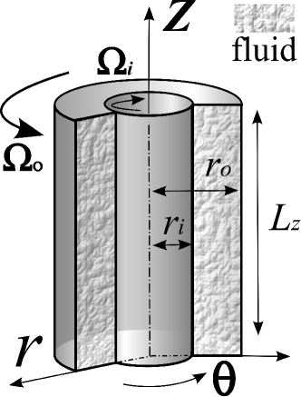
Figure 1: Schematic of the Taylor-Couette system in cylindrical coordinates. The inner and outer cylinder rotate independently with speeds $\Omega_{i}$ and $\Omega_{o}$, respectively. No-slip boundary conditions at the cylinder are used together with axially periodic boundary conditions. The fluid between the cylinders (hatched region) moves by the shear force due to the fluid viscosity.

We solve the equations governing the motion of an incompressible fluid of kinematic viscosity $\nu$ and constant density $\rho$

$$\partial_{t}\textbf{u}+\textbf{u}\cdot\nabla\textbf{u}=-\frac{1}{\rho}\nabla p^{h}+\nu\Delta\textbf{u},\quad\nabla\cdot\textbf{u}=0,$$ (1)

where $\textbf{u}(\textbf{r},t)$ is the velocity field and $p^{h}(\textbf{r},t)$ is the hydrodynamic pressure. Here cylindrical coordinates $\textbf{r}=(r,\theta,z)$ are used. The geometry of the system is shown in Fig. 1 and consists of fluid confined between two concentric cylinders. The inner (outer) cylinder has radius $r_{i}$ $(r_{o})$ and rotates at a speed of $\Omega_{i}$ $(\Omega_{o})$. The Reynolds number in the inner and outer cylinder is defined as $Re_{i,o}=\Omega_{i,o}r_{i,o}d/\nu$, where $d=r_{o}-r_{i}$ is the gap between the cylinders. The geometry is fully specified by two dimensionless parameters: the radii-ratio $\eta=r_{i}/r_{o}$ and the length-to-gap aspect-ratio $\Gamma=L_{z}/d$, where $L_{z}$ is the axial length of the cylinders. At the cylinders no-slip boundary conditions are applied, whereas in the axial direction periodic boundary conditions are imposed to avoid endwall effects. This approximates the case of very long cylinders. In the azimuthal direction periodic boundary conditions occur naturally. However, it is often computationally convenient to simulate only an angular section $L_{\theta}\leq 2\pi$ of the cylinders, and periodic boundary conditions are then used for $\theta\in[0,L_{\theta}]$. This is justified provided that the correlation length of the turbulent flow in the azimuthal direction is shorter than $r_{i}L_{\theta}$ [22].

Henceforth, all variables will be rendered dimensionless using $d$, $\tau=d^{2}/\nu$, and $\nu^{2}/d^{2}$ as units for space, time, and the reduced pressure $p=p^{h}/\rho$, respectively. The Navier-Stokes equations (1) for this scaling become

$$\partial_{t}\textbf{u}+\textbf{u}\cdot\nabla\textbf{u} =-\nabla p+\Delta\textbf{u}$$ (2)

$$\nabla\cdot\textbf{u} =0.$$

In cylindrical coordinates the equations read

$$(\partial_{t}+\textbf{u}\cdot\nabla)u_{r}-u_{\theta}^{2}/r =-\partial_{r}p+\Delta u_{r}-u_{r}/r^{2}-2\partial_{\theta}u_{\theta}/r^{2}$$ (3)

$$(\partial_{t}+\textbf{u}\cdot\nabla)u_{\theta}+u_{\theta}u_{r}/r =-\partial_{\theta}p/r+\Delta u_{\theta}-u_{\theta}/r^{2}+2\partial_{\theta}u_{r}/r^{2}$$

$$(\partial_{t}+\textbf{u}\cdot\nabla)u_{z} =-\partial_{z}p+\Delta u_{z},$$

$$u_{r}/r+\partial_{r}u_{r}+\partial_{\theta}u_{\theta}/r+\partial_{z}u_{z} =0.$$

with $\nabla=(\partial_{r},\partial_{\theta}/r,\partial_{z})$ and $\Delta=\partial_{r}/r+\partial_{rr}^{2}+\partial_{\theta\theta}^{2}/r^{2}+\partial_{zz}^{2}$. Note that the Reynolds numbers enter the system through the boundary conditions

$$u_{\theta}(r_{i,o},\theta,z) =Re_{i,o},$$ (4)

$$u_{r,z}(r_{i,o},\theta,z) =0,$$

$$\textbf{u}(r,\theta,z) =\textbf{u}(r,\theta+L_{\theta},z),$$

$$\textbf{u}(r,\theta,z) =\textbf{u}(r,\theta,z+\Gamma).$$

By taking the divergence of the first equation and then applying the incompressibility condition, we obtain a Poisson equation for the pressure,

$$\Delta p=-\nabla\cdot\textbf{N}(\textbf{u}),\quad\text{where}\quad\textbf{N}(\textbf{u})=\textbf{u}\cdot\nabla\textbf{u},$$ (5)

with consistent boundary conditions [34]

$$\partial_{n}p|_{r=r_{i,o}}=\textbf{n}\cdot[-\partial_{t}\textbf{u}-\textbf{N}(\textbf{u})+\Delta\textbf{u}].$$ (6)

As explained in §3.2, this equation will be solved for the pressure prediction.

3 Numerical Formulation

The governing equations (3) are solved for the primitive variables ($\textbf{u},p$). We discretize the equations with a combination of the Fourier–Galerkin method with the finite-difference method (FD) in space, whereas time is advanced with the semi-implicit fractional-step method of Hugues and Randriamampianina [28], who employ second-order-accurate backward differences with linear (second-order) extrapolation for the nonlinear term. The pseudospectral technique with 3/2-dealiasing is applied to compute the nonlinear term $\textbf{N}(\textbf{u})$ in physical space [11].

3.1 Spatial discretization

In the periodic axial and azimuthal directions, the velocity field and pressure are approximated as

$$\textbf{u}(r,\theta,z)=\sum_{l=-L}^{L}\sum_{n=-N}^{N}\hat{\textbf{u}}^{ln}(r)e^{i(lk_{z}z+nk_{\theta}\theta)},$$ (7)

$$p(r,\theta,z)=\sum_{l=-L}^{L}\sum_{n=-N}^{N}\hat{p}^{ln}(r)e^{i(lk_{z}z+nk_{\theta}\theta)},$$

where $k_{z}$ is the minimum (fundamental) axial wavenumber and fixes the axial non-dimensional length $\Gamma=2\pi/k_{z}$ of the computational domain. Similarly, $L_{\theta}=2\pi/k_{\theta}$ is the azimuthal arc degree; $k_{\theta}=1$ corresponds to the natural periodic boundary condition in the azimuthal direction, whereas $k_{\theta}=4$ corresponds to one quarter of an annulus. The hat symbol $\hat{}$ in (7) denotes quantities in Fourier space and the tuple $(L,N)$ determines the spectral numerical resolution.

By substituting (7) into (3) and projecting the result onto a basis $e^{-i(lk_{z}z+nk_{\theta}\theta)}$ ($l=-L,\dots,L;n=-N,\dots,N$), we obtain the mode-decoupled Navier-Stokes equations. For each Fourier mode $(l,n)$, they read

$$\partial_{t}\hat{u}_{r}+\hat{N}_{r} =-\partial_{r}\hat{p}+\hat{\Delta}\hat{u}_{r}-\hat{u}_{r}/r^{2}-2ink_{\theta}\hat{u}_{\theta}/r^{2},$$ (8)

$$\partial_{t}\hat{u}_{\theta}+\hat{N}_{\theta} =-ink_{\theta}\hat{p}/r+\hat{\Delta}\hat{u}_{\theta}-\hat{u}_{\theta}/r^{2}-2ink_{\theta}\hat{u}_{r}/r^{2},$$

$$\partial_{t}\hat{u}_{z}+\hat{N}_{z} =-ilk_{z}\hat{p}+\hat{\Delta}\hat{u}_{z}.$$

Here $\hat{\Delta}=\partial_{r}/r+\partial_{rr}-n^{2}k_{\theta}^{2}/r^{2}-l^{2}k_{z}^{2}$, and the superscripts $(l,n)$ have been omitted for clarity. Note that the nonlinear term couples Fourier modes and it is thus computed in physical space with the pseudospectral method. Details of the implementation and parallelization of the nonlinear term are given in §4. Equations (8) couple the radial and azimuthal velocities. By applying the following change of variables [35]

$$\hat{u}_{+} =\hat{u}_{r}+i\hat{u}_{\theta},$$

$$\hat{u}_{-} =\hat{u}_{r}-i\hat{u}_{\theta},$$

to equation (8), we obtain the decoupled equations

$$\partial_{t}\hat{u}_{+}(r)+\hat{N}_{+}(r) =-\partial_{r}\hat{p}(r)+nk_{\theta}\hat{p}(r)/r+(\hat{\Delta}-1/r^{2}-2nk_{\theta}/r^{2})\hat{u}_{+},$$ (9)

$$\partial_{t}\hat{u}_{-}(r)+\hat{N}_{-}(r) =-\partial_{r}\hat{p}(r)-nk_{\theta}\hat{p}(r)/r+(\hat{\Delta}-1/r^{2}+2nk_{\theta}/r^{2})\hat{u}_{-},$$

$$\partial_{t}\hat{u}_{z}(r)+\hat{N}_{z}(r) =-ilk_{z}\hat{p}(r)+\hat{\Delta}\hat{u}_{z},$$

where $\hat{N}_{\pm}=\hat{N}_{r}\pm i\hat{N}_{\theta}$.

We use a standard high-order, central finite-difference method to approximate the radial derivatives in equations (9) (see Ref. [36]). The radial nodes are distributed as  [27]

$$r_{j}=\dfrac{1+\eta}{2(1-\eta)}+\dfrac{\sin^{-1}(-\alpha\cos(\pi j/M))}{2\,\sin^{-1}\alpha},\qquad j=0,\dots,M.$$ (10)

For $\alpha=1$ the grid is uniform, whereas for $\alpha\rightarrow 0$ the Chebyshev collocation points are obtained. Here stencils of $n_{s}=9$ points, corresponding to a scheme of formally order 8 was found to give the best compromise in our tests. Note that we reduce the stencil length gradually towards the boundaries in order to keep the FD-matrices banded. We show in §5 that due to the clustering of nodes near the walls with typical values of $\alpha=0.5$ this reduction of the order of accuracy does not produce a larger error at the boundaries.

With $(L,N)$ Fourier modes and $M$ radial nodes, the number of grid points in physical space is $(n_{r},n_{\theta},n_{z})=(M,2N+1,2L+1)$ in the radial, azimuthal and axial directions, respectively. Note that we dealiase the nonlinear term by computing it on a grid of $(M,3N+1,3L+1)$ points.

3.2 Temporal scheme

A stiffly stable temporal scheme based on a backward differentiation formula with extrapolation for the nonlinear term is adopted (see Ref. [28, 37]). It reads

$$\frac{3\textbf{u}^{i+1}-4\textbf{u}^{i}+\textbf{u}^{i-1}}{2\Delta t}+2\textbf{N}^{i}(\textbf{u})-\textbf{N}^{i-1}(\textbf{u})=-\nabla p^{i+1}+\Delta{\textbf{u}^{i+1}}.$$ (11)

In the literature this is often referred to as Adams-Bashforth backward-difference method of second order (AB2BD2). The viscous terms are discretized implicitly, whereas the nonlinear terms are treated explicitly. At each time step, equation (11) is solved through a fractional step method proposed by Hugues and Randriamampianina [28]. The method is summarized below. Here $(\hat{\textbf{u}}^{i},\hat{p}^{i})$ denote the spectral coefficients at the $i^{th}$ time step.

1. Obtain spectral coefficients of the nonlinear term, $\hat{\textbf{N}}^{i}(\textbf{u})$, using the 3/2-dealiasing rule

   • Do matrix-vector multiplication to calculate $\partial_{r}\hat{\textbf{u}}^{i}$ (FD method)

   • Compute dot product in Fourier space to calculate $\partial_{\theta}\hat{\textbf{u}}^{i}$ and $\partial_{z}\hat{\textbf{u}}^{i}$

   • Perform Fourier transform of $\partial_{r,\theta,z}\hat{\textbf{u}}^{i}$ and $\hat{\textbf{u}}^{i}$ to obtain the velocity field and all its derivatives in physical space;

   • Calculate $\textbf{N}^{i}(\textbf{u})=\textbf{u}^{i}\cdot\nabla\textbf{u}^{i}$;

   • Perform inverse Fourier transform to obtain the spectral coefficients $\hat{\textbf{N}}^{i}(\textbf{u})$.

2. Obtain the pressure prediction, $\hat{p}^{*}$: solve the Poisson equation

   $$\Delta\hat{p}^{*}=\nabla\cdot[-2\hat{\textbf{N}}^{i}(\textbf{u})+\hat{\textbf{N}}^{i-1}(\textbf{u})],$$ (12)

   with consistent Neumann boundary conditions (6).

3. Obtain the velocity prediction, $\hat{\textbf{u}}^{*}$: solve the three Helmholtz equations

   $$\frac{3\hat{\textbf{u}}^{*}-4\hat{\textbf{u}}^{i}+\hat{\textbf{u}}^{i-1}}{2\Delta t}+2\hat{\textbf{N}}^{i}(\textbf{u})-\hat{\textbf{N}}^{i-1}(\textbf{u})=-\nabla\hat{p}^{*}+\Delta\hat{\textbf{u}}^{*}$$ (13)

   with Dirichlet boundary conditions (4).

4. Correct via an intermediate variable $\phi=2\Delta t(\hat{p}^{i+1}-\hat{p}^{*})/3$. The incompressibility condition $\nabla\cdot\hat{\textbf{u}}^{i+1}=0$ leads to a Poisson equation for $\phi$ with homogeneous Neumann boundary conditions (see Ref. [34, 28])

   $$\Delta\phi=\nabla\cdot\hat{\textbf{u}}^{*},$$ (14)

   $$\partial_{r}\phi|_{r=r_{i,o}}=0$$

5. Compute pressure and velocity correction, $\hat{p}^{i+1}$ and $\hat{\textbf{u}}^{i+1}$:

   $$\hat{p}^{i+1} =\hat{p}^{*}+3\phi/(2\Delta t)$$ (15)

   $$\hat{\textbf{u}}^{i+1} =\hat{\textbf{u}}^{*}-\nabla\phi$$

6. Go back to step 1

The Navier-Stokes equations are thus advanced in time by solving five systems of linear equations (12)-(14), of Poisson or Helmholtz type, for each Fourier mode. This method accounts for a divergence-free velocity field and a small slip at the wall of the order of $\mathcal{O}(\Delta t^{3})$ in the tangential velocities, $u_{z}$ and $u_{\theta}$. We note that the method was originally developed and tested [28] for the two-dimensional Navier-Stokes equation discretized on a Chebyshev-Chebyshev collocation grid, and the Poisson and Helmholtz equations were solved using the double diagonalization method, thus rendering quadratic computational complexity in each direction. Here, the FD-discretized Poisson and Helmholtz equations render banded matrices which are solved with the LU-method. The decompositions are precomputed at the beginning of a simulation and at each time step only backward and forward substitutions need to be computed, resulting in an operation count of $\mathcal{O}(M)$ for the solution of each system. Note that for the axially and azimuthally invariant Fourier mode, $n=l=0$, the Poisson equations (12) and (14) are singular: their solution is defined up to a constant because of the Neumann boundary conditions. Here a Dirichlet homogeneous boundary condition was employed at the outer cylinder to select a particular solution.

4 Parallelization scheme and its implementation

A hybrid MPI-OpenMP parallelization strategy is adopted for the implementation of the code. Since the linear equations (12)–(14) are mode-independent, it is convenient to employ an MPI-based, one-dimensional domain decomposition (also known as “slab” decomposition, Fig. 2): The Fourier coefficients $(\hat{u}_{+},\hat{u}_{-},\hat{u}_{z},\hat{p})$ corresponding to different modes are distributed across the MPI tasks, which allows to solve equations (12)–(14) concurrently, without inter-task communications. Each of the $N_{\mathrm{tasks}}$ MPI tasks operates on data corresponding to a number of $m_{\theta}\cdot m_{z}/N_{\mathrm{tasks}}$ modes, where $(m_{r},m_{\theta},m_{z})=(M,N+1,2L)$ are the dimensions of variables in Fourier space. OpenMP threading inside each MPI task allows to efficiently exploit the remaining coarse-grained parallelism (see below).

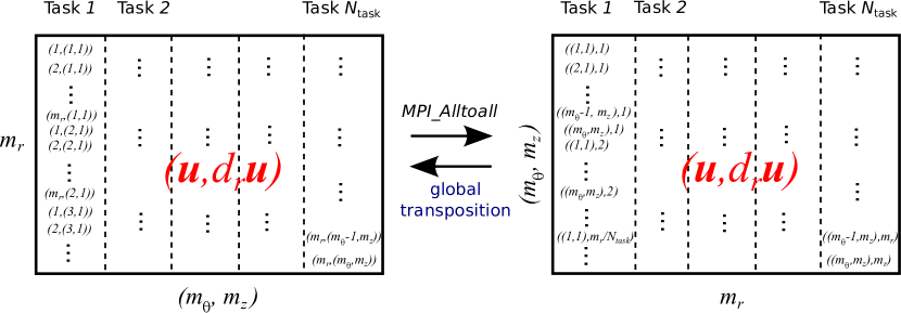
Figure 2: Schematic of the MPI-based, one-dimensional “slab” domain decomposition and the global transposition by using the function MPI_Alltoall(). Mode-independent spectral coefficients in Fourier space are distributed among different MPI tasks. Each variable has a dimension of $(m_{r},m_{\theta},m_{z})$.

We compute the nonlinear term (step 1 in Section 3.2) by performing global matrix transpositions (Fig. 2) of the discretized fields $\partial_{r}\hat{\textbf{u}}$ and $\hat{\textbf{u}}$ such that for each radial point the complete spectrum of Fourier modes is localized in one MPI task. This requires a collective communication operation of type ”all-to-all” but allows to most efficiently compute the Fourier transformations and the derivatives with respect to the spectral coordinates, namely $\theta$ and $z$. Finally, inverse transpositions are performed for the resulting array $\hat{\textbf{N}}$.

In our applications, typically $m_{\theta}\cdot m_{z}\gg m_{r}$ applies, i.e. there are many more Fourier modes than radial grid points. Hence, the number of MPI tasks in our slab decomposition is bounded by $N_{\mathrm{tasks}}\leq m_{r}$ (cf. Fig.. 2) and consequently the achievable parallel speedup with respect to the serial code would be at most $m_{r}$. However, OpenMP threads allow to parallelize over the $m_{\theta}\cdot m_{z}/N_{\mathrm{tasks}}$ modes within a MPI task, while retaining the one-dimensional MPI domain decomposition, which is conceptually straightforward to implement. Similarly, we can exploit concurrency in the nonlinear part if $N_{\mathrm{tasks}}<m_{r}$ applies. In addition, the Fourier transformations and the individual partial derivatives required for evaluating $\textbf{u}\cdot\nabla\textbf{u}$ are computed concurrently and the transposition of $\partial_{r}\hat{\textbf{u}}$ is overlapped with the computation of u, $\partial_{\theta}\textbf{u}$, and $\partial_{z}\textbf{u}$.

Theoretically, this strategy allows to utilize a number of $\min(m_{r},m_{\theta}\cdot m_{z})\cdot N_{\mathrm{threads}}$ processor cores where $N_{\mathrm{threads}}$ is the maximum number of threads a shared-memory compute node provides. Current high performance computing (HPC) platforms feature at least 16 cores with 32 logical threads per node (e.g. Intel Xeon E5 Sandy-Bridge or Ivy-Bridge processors), and thread-based concurrency on the node-level is expected to increase substantially in the near future, in particular with the many-core processors and GPU-accelerated nodes [38]. In practice, we achieve the best parallel efficiencies when MPI tasks are mapped to the individual ”sockets” (i.e. CPUs or NUMA domains) of a compute node and the number of OpenMP threads equals the number of physical cores per socket. Due to the smaller number of MPI tasks per node (compared with a plain MPI parallelization) the amount of inter-node communications is reduced in the global transposition. This transposition, which is implemented by MPI_Alltoall collective communication and task-local transpositions, ultimately limits the overall parallel scalability of the code at high task counts (see Section 6).

The code is implemented in FORTRAN 90 and has been ported to a number of major HPC architectures, including IBM Power and BlueGene, as well as compute clusters based on x86_64 processors and high-performance interconnects such as InfiniBand. We employ vendor-optimized BLAS and LAPACK routines for the matrix-vector multiplication (BLAS level-2 routine DGEMV) and the linear solvers (LAPACK routines DGBTRF, DGBTRS taken e.g. from the Intel Math Kernel Library, MKL, or IBM ESSL), respectively, and utilize the MKL or the FFTW library [39] for performing the Fourier transformations in the nonlinear part of the code. For data output we employ the parallel HDF5 libraries which enable collective output of the MPI-distributed data into a single file in a transparent and efficient way. This facilitates data handling, post-processing and visualization, e.g. with VisIT or Paraview (cf. Fig. 9).

5 Numerical Accuracy and Code Validation

The code has been tested over a wide range of Reynolds numbers $Re\in[50,100\,000]$. A number of specific test cases will be given in the following.

5.1 Laminar flow

We firstly computed the laminar velocity profile, which is also known as circular Couette flow. It can be expressed as $\textbf{U}=(0,U_{\theta}(r),0)$, where $U_{\theta}(r)=C_{1}r+C_{2}/r$ with $C_{1}=(Re_{o}-\eta Re_{i})/(1+\eta)$ and $C_{2}=\eta(Re_{i}-\eta Re_{o})/((1-\eta)(1-\eta^{2}))$, and corresponds to pure rotary shear flow. The tests were performed at $Re_{i}=50,Re_{o}=200$ and at $\eta=0.5$.

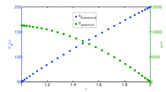
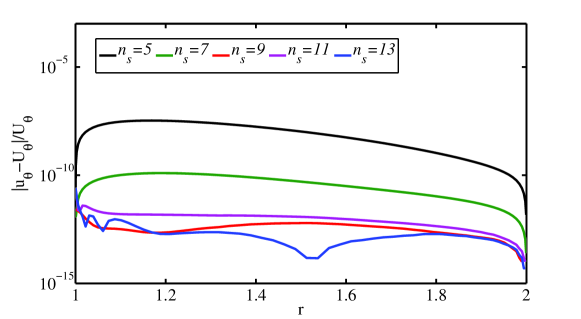
Figure 3: Laminar Couette flow at $Re_{i}=50,Re_{o}=200$ and $\eta=0.5$ with Chebyshev points ($\alpha\rightarrow 0$ in equation (10)). Top: numerically obtained streamwise velocity profile (blue squares) and pressure (green circles) for $n_{r}=32$. The dashed lines show the corresponding curves for the exact Couette solution. Bottom: local relative error $\epsilon_{u}$ for $n_{r}=64$ as a function of $r$ and several stencil lengths $n_{s}$.

A non-uniform grid according to formula (10) was used in the radial direction. Fig. 3(top) shows the numerical velocity and pressure profiles for $\alpha\rightarrow 0$ (Chebyshev points) and $n_{r}=32$, which match well with the theoretical curves (dashed lines). The distributions of the relative error $\epsilon_{u}(r)=|\frac{u_{\theta}-U_{\theta}}{U_{\theta}}|$ along the radial direction are shown in Fig. 3(bottom) for $n_{r}=64$ and different stencil lengths $n_{s}$. In the FD method, the stencil length is the number of consecutive points used to approximate the derivatives. As $n_{s}$ is increased, the relative error decreases until approaching the machine precision. We found that a stencil of 9 points gives a good compromise between computing time and accuracy, so $n_{s}=9$ is kept for the following tests.

To measure the global error, we integrated the local error $\epsilon_{u}$ over the radial direction, $\mathcal{E}_{u}=\int_{r_{i}}^{r_{o}}\epsilon_{u}rdr$. This is shown in Fig. 4 as a function of $n_{r}$ and $\alpha$. In the left panel, $\mathcal{E}_{u}$ scales as a power law with $n_{r}$ for both $\alpha=0$ and $\alpha=0.5$. The power exponent is about $-11$, which is better than expected from the 9-point-stencil FD scheme. The right panel shows that the error is minimized for $\alpha\simeq 0.5$ and that below 0.5 the errors are almost at the same level.

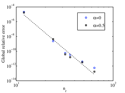
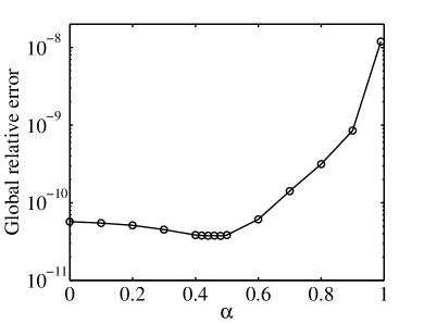
Figure 4: Global relative error $\mathcal{E}_{u}$ as a function of $n_{r}$ (left) and $\alpha$ for $n_{r}=32$ (right). The dashed line in the left panel is a power fit with an exponent of -11. The stencil length is $n_{s}=9$ in both panels.

5.2 Hydrodynamic instability and three-dimensional time-dependent flow

As the Reynolds number of the inner cylinder increases beyond a certain value, laminar Couette flow gives way to Taylor vortices, and subsequently to wavy vortex flow. Following Jones [40] we computed the onset of wavy vortex flow for $\eta=0.56$, $\Gamma=2.2$ and $k_{\theta}=1$. The simulations were initialized with Taylor vortex flow, which was disturbed with a perturbation of azimuthal wavenumber $n$. We then measured the exponential growth/decay rate of the kinetic energy of the disturbed mode, which vanishes at the critical point. In agreement with Jones we found that the dominant mode has $n=1$. The critical Reynolds number, obtained with $(n_{r},n_{\theta},n_{z})=(64,48,128)$ and $\Delta t=2\times 10^{-5}$, was determined to $Re_{i}^{c}\in[408.09,408.1]$, which was reproduced by using the Petrov–Galerkin code of Meseguer et al. [26]. We note that Jones quotes a slightly lower value (399, Table 1 of [40]). We attribute this discrepancy of about 2% to the limited axial and radial resolutions, which Jones could use in the eighties.

Nonlinear time-dependent wavy vortex flow was computed at $Re_{i}=458.1,Re_{o}=0$, $\eta=0.868$ and is shown in Fig. 5. The axial length was chosen as $\Gamma=2.4$ and $k_{\theta}=6$ to compare to the experimental observations of King et al. [41] and numerical simulations of Marcus [24]. Wavy Taylor vortices are a relative equilibrium: they consist of a constant pattern rotating as a solid at a constant wave speed. Marcus [24] notes: ‘A test that is more sensitive than the comparison of torques is the comparison of the numerically computed wave speed with the experimentally observed wave speed’. We performed this test with spatial resolution $(n_{r},n_{\theta},n_{z})=(32,32,32)$ and time-step size $\Delta t=2\times 10^{-5}$. The wave speed normalized by the rotation speed of the inner cylinder was accurately computed with a rigorous method based on Brent’s minimization algorithm [42]. Our result, namely a wave speed of $c=0.34432$, with the pattern rotating at about one-third of the speed of the inner cylinder, agrees to all decimal places given in [41]. The same result was reproduced with higher resolutions (as in §5.3) and on various HPC platforms.

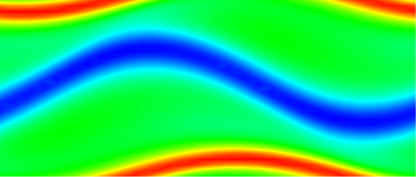
Figure 5: Contour plots of the streamwise velocity in the middle $(\theta,z)$ plane for wavy Taylor vortices. The outer cylinder is stationary, whereas the inner cylinder rotates with $Re_{i}=458.1$. The geometrical parameters are $\eta=0.868$ and $\Gamma=2.4$ and only one sixth of the circle ($k_{\theta}=6$) was used in the simulations and is displayed. Here $(n_{r},n_{\theta},n_{z})=(32,32,32)$.

The choice $k_{\theta}=6$, as in [24], automatically fixes the symmetry of the observed wavy mode. To remove this constraint, we did an extra set of simulations with $k_{\theta}=1$, i.e. the whole annulus in the azimuthal direction. After initial transients the flow stabilized to a wavy state, whose wavenumber and speed depended on the disturbance used to initialize the run. When a disturbance with $n=6$ was used, exactly the same result as above was obtained. We also tried $n=5$ an $n=7$ and obtained new wavy-vortex-flow sates, all of which had very similar wavespeed. The same results were reproduced by doubling the axial length of the domain, i.e. $\Gamma=4.2$, and for much longer cylinders ($\Gamma=14.4$). Finally, we note that for other disturbances, which simultaneously excited several modes, we could also obtain chaotic flow states. Overall, the results are in agreement with the experiments of Coles [43], who demonstrated the coexistence of several flow states at identical parameter values depending on the history of the flow. An investigation of the basin of attraction of each of the possible flow states would be very interesting and may be pursued in the future. We expect extreme multiplicity, much beyond what Coles observed.

5.3 Velocity slip at the cylinders

We further examined the tangential velocity slip at the cylinders. In the projection scheme we employed, the incompressibility constraint $\nabla\cdot\textbf{u}=0$ is discretely fulfilled by construction, in that the Poisson equation for $\phi$ in §3.2 is derived by applying the divergence-free condition. However, the velocities at the inner and outer cylinders slip by a predicted amount of $|\nabla\phi|=\mathcal{O}(\Delta t^{3})$ after the correction step [28, 29]. We have evaluated the L2-norm of the tangential velocity slip at the inner cylinder, $\int_{\theta}\int_{z}\sqrt{((u_{\theta}-Re_{i})^{2}-u_{z}^{2})|_{r=r_{i}}}d\theta dz$. In Fig. 6 the relative velocity slip, i.e. slip velocity normalized with $Re_{i}$, is shown as a function of $\Delta t$ for several radial resolutions $n_{r}$. For the lowest resolution $n_{r}=32$ the curve rapidly levels off, indicating that spatial-discretization errors dominate over temporal errors. Note that with the largest time-step size allowed for stability and lowest resolution we already obtain five digits in the accuracy of $c$. As $n_{r}$ is increased the slip velocity decreases and its scaling gradually approaches a power law, here with an exponent of approximately 2.5. The reason why this is slightly below the predicted value of $3$, as observed by Raspo et al. [29] for simple cosine and sine flows, is unclear. The behaviour seen in Fig. 6 suggests that very high spatial resolutions may be needed to observe the asymptotic scaling. Nevertheless we stress that the even with the coarsest resolution and time step, the relative slip error is of about $10^{-6}$. We repeated this study for fully turbulent flow at $Re_{i}=8000$ (see §5.5 for further tests with the same setup). The results were very similar, and in fact, even with $\Delta t=2\times 10^{-7}$, which is close to the stability limit ($\Delta t_{\text{lim}}\approx 3\times 10^{-7}$), the relative error was $10^{-9}$. We conclude that in typical simulations the dominating source of error comes from the spatial discretization, which determines the slip error observed in practice. A time step moderately smaller than permitted by stability yields very accurate results in the solution and very small slip velocities.

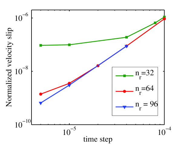
Figure 6: Normalized velocity slip at the inner cylinder versus time-step size $\Delta t$ for different $n_{r}$. The parameters are the same as in Figure 5, corresponding to wavy vortex flow. The spatial resolution in the axial and azimuthal directions is $(n_{\theta},n_{z})=(32,32)$

5.4 Localized turbulence at moderate Re

Localized turbulence, interspersed in the surrounding laminar flow, is a typical feature of transitional Reynolds numbers in shear flows. The turbulent stripe pattern found in the counter-rotating Taylor-Couette flow in the narrow-gap limit is an example. We computed this pattern for exact counter-rotation ($Re_{i}=-Re_{o}=680$) and $\eta=0.993$. The time-step size was $\Delta t=2\times 10^{-5}$ and the domain size in the axial direction was $\Gamma=50$, whereas $k_{\theta}=179$. Folowing Barkley and Tuckermann [44] the $\theta$-direction in our computational domain is tilted with an angle of $24^{\circ}$ to the streamwise direction (for details see [45]). We tested the probability distributions of the splitting times of turbulent stripes reported in [45], which were obtained by using the spectral Petrov-Galerkin code of Meseguer et al. [26]. We here used $n_{r}=32$ in the radial direction, whereas Shi et al. [45] used modified Chebyshev polynomials of degree up to 26. In both cases the azimuthal and axial resolutions are $n_{\theta}=48$ and $n_{z}=640$, respectively. The exponential distributions of splitting times obtained by both codes are statistically equivalent (see the inset in Fig. 7): our computed characteristic time of the exponential distributions is well within the $95\%$ confidence interval reported in [45].

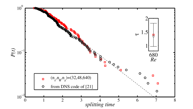
Figure 7: Probability distributions of the splitting time of a single turbulent stripe at $Re_{i}=680,Re_{o}=-680$ and at $\eta=0.993$. Circles correspond to the data set obtained with the spectral Petrov–Galerkin code of Meseguer et al. [26], whereas squares correspond tot the data set obtained with the present code with $(n_{r},n_{\theta},n_{z})=(32,48,640)$. Inset: characteristic splitting time estimated with the sample mean. The error bar shows the $95\%$ confidential interval.

5.5 Fully turbulent flow at high Re

The robustness of the code was further validated at high Reynolds numbers in the linearly unstable regime, where the flow is fully turbulent. Here we computed the global torque exerted by the fluid on the inner and outer cylinders, which characterizes the turbulence intensity and the transport of angular momentum [22]. The tests were done at $Re_{i}=8000$ and stationary outer cylinder with $\eta=0.5$, $\Gamma=2\pi/k_{z}=\pi$ and $k_{\theta}=2$. The time-step size is $\Delta t=2\times 10^{-7}$. As is shown in Fig. 8(top), the quasi-Nusselt number $Nu_{\omega}$ [22], which is the torque normalized by the torque of the laminar flow, converges to $8.815$ at the resolution $(n_{r},n_{\theta},n_{z})=(128,192,320)$. This value agrees very well to the value of $8.816$ recently reported by Brauckmann and Eckhardt [22], who also used the spectral Petrov-Galerkin code of Meseguer et al. [26]. The temporal fluctuation of the quasi-Nusselt number obtained with the highest resolution is shown in the bottom figure. At this $Re$, we also examined the influence of the radial node distribution by varying the parameter $\alpha$ in equation (10). Three runs with $\alpha=0,0.5,0.99$ were done, and all three rendered $Nu_{\omega}=8.81\pm 0.05$. The maximum time-step size for stability was found to be $\Delta t_{\text{lim}}\approx 3\times 10^{-7}$ for all three values of $\alpha$. This is explained by the fact that the CFL number is dominated by the azimuthal direction. Thus at this Reynolds number the Chebyshev node distribution does not impose a restriction in the time-step yet.

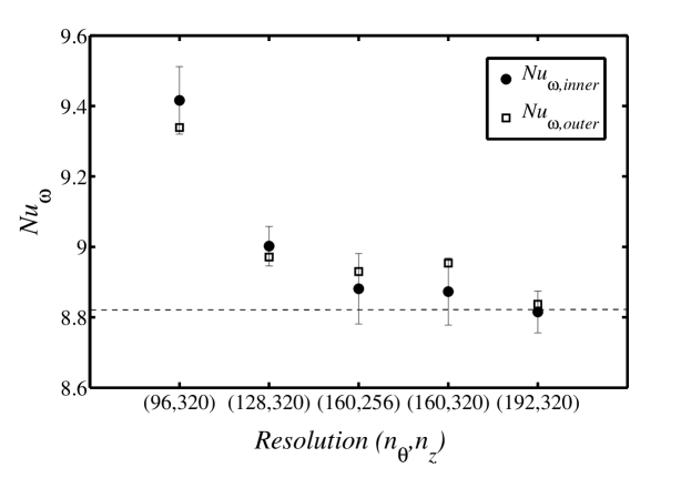
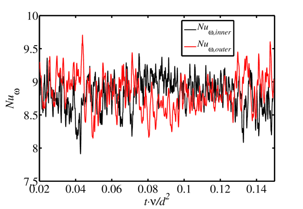
Figure 8: (Top) Quasi-Nusselt number at $Re_{i}=8000$, $Re_{o}=0$, $\eta=0.50$, $\Gamma=2\pi/k_{z}=\pi$ and $k_{\theta}=2$, as a function of the azimuthal and axial resolutions for $n_{r}=128$. The dashed line corresponds to the value ($Nu_{\omega}\simeq 8.816$) reported in [22]. The error bars indicate the $95\%$ confidential interval. (Bottom) The temporal fluctuation of the quasi-Nusselt number at the highest resolution $(n_{r},n_{\theta},n_{z})=(128,192,320)$.

Another test run was performed at $Re_{i}=10^{5},Re_{o}=79685$ and at $\eta=0.71$. We used $k_{\theta}=16$ and axial length $\Gamma=0.5$, with a spatial resolution $(n_{r},n_{\theta},n_{z})=(1152,384,384)$ and time-step size $\Delta t=10^{-9}$. The initial condition at $t=0$ is taken from the optimal initial perturbation, which gives the maximal transient energy growth [46] supplemented with very small three-dimensional noise. Fig. 9 shows the 3D contour plot of the streamwise vorticity, $\omega_{\theta}=\partial_{z}u_{r}-\partial_{r}u_{z}$, at $t=5\times 10^{-4}$ ($\simeq 3.3$ cylinder rotations) which illustrates a transiently turbulent flow state. The research is still ongoing and will be disseminated in future publications. We expect that the results will contribute to clarify the role of pure hydrodynamic turbulence in astrophysical disks [2].

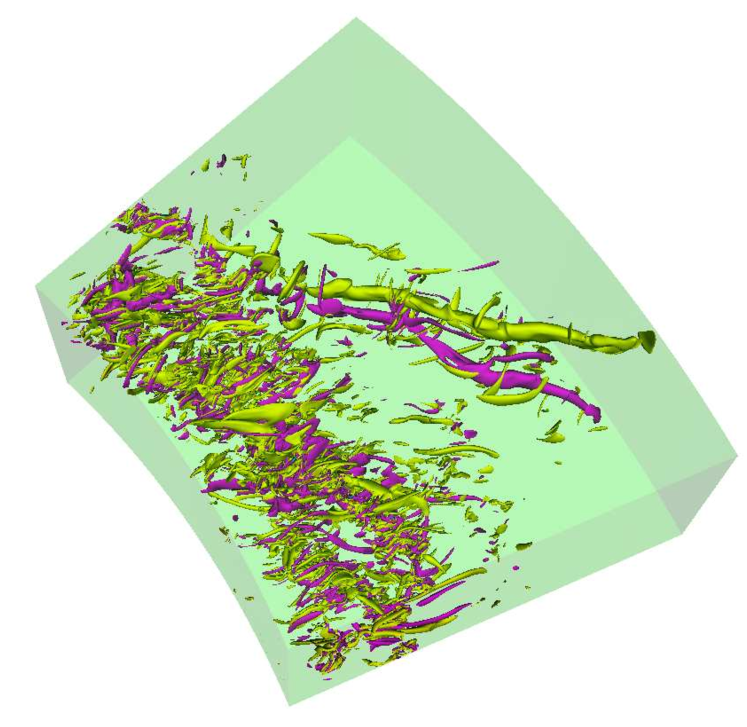
Figure 9: Isosurfaces of the streamwise vorticity in the quasi-Keplerian regime at $Re_{i}=10^{5},Re_{o}=79685$, $\eta=0.71$, $\Gamma=0.5$ and $k_{\theta}=16$. The resolution is $(n_{r},n_{\theta},n_{z})=(1152,384,384)$.

6 Computational efficiency

6.1 Benchmark setup

In this section we report benchmarks results using up to 20 480 processor cores of an IBM iDataPlex compute cluster with Intel Ivy-Bridge processors and a fully nonblocking InfiniBand (FDR 14) fat-tree interconnect. Each shared-memory compute node hosts two Intel Xeon E5-2680v2 ten-core processors (CPUs) with a clock frequency of 2.8 GHz. We employ Intel compilers (version 14.0), and the Intel Math Kernel Library (MKL 11.1) for BLAS, LAPACK, and FFT functionality. We have performed two strong scaling studies, which show the scaling of the runtime with increasing number of CPU cores for a fixed problem size. Two different, representative setups were considered:

1. a “SMALL” setup with $(n_{r},n_{\theta},n_{z})=(32,384,640)$. This setup is used to investigate localized turbulence at the transitional stage ($Re\sim\mathcal{O}(10^{2})$), where the structures inside the turbulence are relatively large. The probability distributions of the splitting time of localized turbulent stripe in §5.4 are obtained with this resolution.

2. a “LARGE” setup with $(n_{r},n_{\theta},n_{z})=(2048,384,2048)$. This resolution is representative of our ongoing studies of hydrodynamic turbulence in Taylor-Couette flows with quasi-Keplerian velocity profiles at Reynolds numbers up to $\mathcal{O}(10^{5})$.

For the LARGE setup, a weak scaling study, i.e. increasing the problem size along with the number of CPU cores, is presented in addition.

6.2 Benchmark results and discussion

Fig. 10 provides an overview of the strong scalability of the hybrid code. Different colors and symbols are used to distinguish runs with different numbers of MPI tasks ($N_{\mathrm{tasks}}$) and OpenMP threads ($N_{\mathrm{threads}}$). The total number of processor cores is given by $N_{\mathrm{cores}}=N_{\mathrm{tasks}}\cdot N_{\mathrm{threads}}$.

For both setups we achieve scalability up to the maximum number of cores our parallelization scheme admits on this computing platform, i.e.,  $N_{\mathrm{cores}}=32\cdot 20=640$ for the SMALL setup, and $N_{\mathrm{cores}}=2048\cdot 10=20480$ for the LARGE setup. The latter number is constrained by the maximum number of nodes that can be used by a single job.

For the SMALL setup, Fig. 10 (upper left) shows that up to a number of 10 threads per MPI task the run times for a given number of cores are virtually the same, independent of the distribution of the resources to MPI tasks and OpenMP threads. This indicates that the efficiency of our coarse-grained OpenMP parallelization is almost the same as the explicit, MPI-based domain decomposition. Moreover, as the results for the LARGE setup (Fig. 10, upper right) show, it can even be more efficient to use less than the maximum of $n_{r}$ MPI tasks for a given number of cores and utilize the resources with OpenMP threads (compare the cyan and the red symbols at moderate core counts). This is due to the fact that a lower number of MPI tasks per node reduces the amount of inter-node MPI communication (specifically the MPI_Alltoall communication pattern for the global transpositions). Notably, for the LARGE setup, the hybrid code shows nearly perfect scaling between 1280 and 2560 cores and continues to scale up to more than 20 000 processor cores (1024 nodes), albeit with a marginally efficient speedup of 8 (corresponding to a parallel efficiency of slighly more than 50%) when compared with the baseline run at 1280 cores. A floating-point performance of about 20 GFlop/s per compute node is reached which is roughly 5% of the nominal peak performance. The memory footprint remains below 10 GB per node, making the code well prepared for future CPU architectures with scarce memory resources [38].

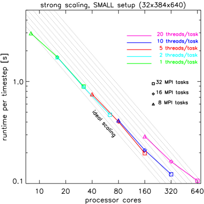
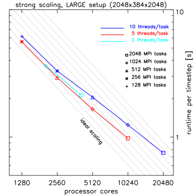
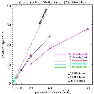
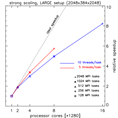
Figure 10: Runtime per time step (upper row) and relative speedups (bottom row) for the SMALL setup (left panels) and for the LARGE setup (right panels) as a function of the number of cores, $N_{\mathrm{cores}}=N_{\mathrm{tasks}}\cdot N_{\mathrm{threads}}$. Different colors and symbols are used to distinguish runs with different numbers of MPI tasks ($N_{\mathrm{tasks}}$) and OpenMP threads ($N_{\mathrm{threads}}$), respectively. The slope of an ideal scaling curve is indicated by dotted lines.

The details on the absolute run times and the parallel efficiencies of the whole code (the bottom row) as well as the individual parts of the algorithm (cf. Section 3.2) are listed in Table 1. The first column, which corresponds to a plain MPI-parallelization using the maximum number of tasks ($N_{\mathrm{tasks}}=n_{r}$) for the given setup, is assigned an efficiency of 100%, by definition.

SMALL setup $(32,384,640)$
cores ($N_{\mathrm{threads}}$)	$32(1)$		$64(2)$		$160(5)$		$320(10)$		$640(20)$
	$T_{1}$ [s]	$\eta$	$T_{2}$ [s]	$\eta$	$T_{5}$ [s]	$\eta$	$T_{10}$ [s]	$\eta$	$T_{20}$ [s]	$\eta$
nonlinear (1)	0.696	100%	0.388	90%	0.161	86%	0.101	69%	0.093	37%
predictor-corrector (2,3,4)	0.152	100%	0.080	95%	0.033	92%	0.017	89%	0.001	79%
complete step	0.864	100%	0.472	92%	0.200	86%	0.120	72%	0.104	42%
LARGE setup $(2048,384,2048)$
cores ($N_{\mathrm{threads}}$)	$2048(1)$		$4096(2)$		$10240(5)$		$20480(10)$
	$T_{1}$ [s]	$\eta$	$T_{2}$ [s]	$\eta$	$T_{5}$ [s]	$\eta$	$T_{10}$ [s]	$\eta$
nonlinear (1)	3.875	100%	1.862	104%	0.870	89%	0.695	70%
predictor-corrector (2,3,4)	0.407	100%	0.240	85%	0.097	84%	0.048	85%
complete step	4.325	100%	2.134	101%	0.977	87%	0.751	58%

Table 1: Runtime per time step, $T_{n}$ and parallel efficiency $\eta$ of the OpenMP parallelization as a function of the number $N_{\mathrm{threads}}$ of OpenMP threads per MPI task, using the maximum number of 32 MPI tasks for the SMALL setup, and 2048 MPI tasks for the LARGE setup, respectively. Parallel efficiency is conventionally defined as $\eta:=T_{1}/(n\cdot T_{n})$ with $n=N_{\mathrm{threads}}$. Different rows show the contributions of the individual algorithmic steps (numbering in brackets chosen according to Section 3.2) to the total runtime of a complete time step (the bottom row).

For the SMALL setup (the upper part of Table 1) we observe good OpenMP efficiency up to 10 threads (which are pinned to the 10 physical cores of a single CPU socket) per MPI-task for the pressure and velocity predictor steps, the corrector step, and also the matrix-vector multiplication in the nonlinear part. When using all 20 cores of a shared-memory node with a single MPI task (cf. the magenta curve in Fig. 10, left) one notices a degradation in OpenMP efficiency which is due to memory-bandwidth limitations, NUMA effects, and limited parallelism in the nonlinear part. The overall parallel efficiency (the bottom row) can be considered as very good up to 320 cores, but gets increasingly bounded by the global transposition (MPI_Alltoall communication) in the nonlinear part.

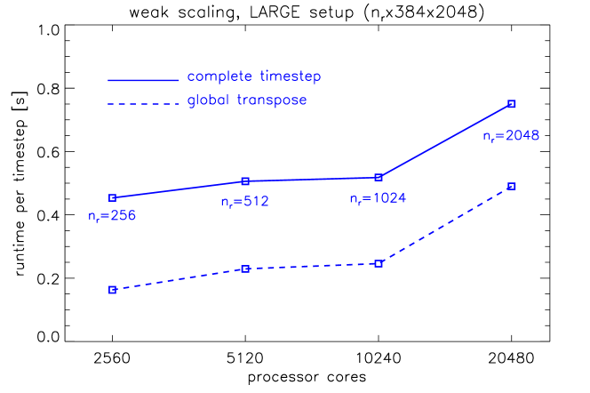
Figure 11: Weak scaling of the total runtime (solid line) and the contribution of the global transposition (dashed) for the LARGE setup. The number of cores is related to the number of radial zones as $N_{\mathrm{cores}}=10\cdot n_{r}$. In all cases, $N_{\mathrm{threads}}=10$ was used.

For the LARGE setup (the lower part of Table 1), although the highly scalable linear parts (predictor-corrector, steps 2-4) and the matrix-vector multiplications contribute only a minor part to the total runtime, the code maintains an excellent OpenMP efficiency up to more than 10 000 cores (87%). At very high core counts the MPI_Alltoall communication dominates the total runtime and becomes the major bottleneck for overall scalability. This is also apparent in the weak scaling analysis (cf. Fig. 11). The global transposition exhibits good weak scalability up to 10 240 cores (512 nodes), and its contribution to the total runtime remains subdominant but it seriously impedes the scalability up to the maximum of 20 480 cores (1024 nodes). Note that parts of the global transposition (roughly a third, in terms of runtime) are performed concurrently with computations and are thus not accounted for separately in Fig. 11.

Using an adapted setup of $(n_{r},n_{\theta},n_{z})=(1792,384,512)$, we were able to run the code on the largest, fully interconnected partition with 1792 nodes (35 840 cores) of the high-performance computer of the Max-Planck-Society, ”Hydra”, resulting in a run time of $0.3$ s per time step. Computing times of this order enable us to perform highly resolved simulations (e.g. of Keplerian flows which require on the order of a million time steps) within a couple of days.

7 Conclusion

With the motivation of exploring high-Reynolds-number rotating turbulent flows, we developed a highly-efficient parallel DNS code for Taylor-Couette flows. The incompressible Navier-Stokes equations in cylindrical coordinates are solved in primitive variables by using a projection method proposed by Hugues and Randriamampianina [28], which is second-order accurate in both pressure and velocity. This method leads at each time step to the solution of five linear differential equations, either of Poisson or of Helmholtz type, which simplifies significantly the programming of the code. For the spatial discretization, we used a combination of Fourier spectral in axial and azimuthal directions and high-order finite differences in the radial direction, which allow the use of tailored stretched grids. The computing cost scales linearly with the number of grid points in each direction.

In order to reach higher Reynolds numbers and to take full advantage of the modern HPC facilities, the code was parallelized by a hybrid MPI-OpenMP strategy, combining the simplicity of a MPI-based one-dimensional “slab” domain decomposition in Fourier space with efficient exploitation of the remaining coarse-grained parallelism by OpenMP threading. Compared to a flat MPI-parallelization, the hybrid code maps more naturally to the current multi-node, multi-core architectures, keeps the number of MPI tasks in the well-manageable regime of a few thousand, and, most importantly, reduces inter-node communications, which improves the overall efficiency and scalability. The strong scaling study which was performed with scientifically relevant setups demonstrates the scalability of the code up to more than 20 000 processor cores. This allows to perform simulations with much higher resolutions than previously possible. With the current HPC technology, this code pushes the achievable $Re$ to the order of magnitude of $\mathcal{O}(10^{5})$ in DNS of Taylor-Couette flow, which therefore opens up the possibility to study quasi-Keplerian flows at experimentally relevant parameters.

The new code was shown to be very accurate in various regimes: laminar Couette flow, wavy vortices, transitional and turbulent flow at high Reynolds number. With the high efficiency of the hybrid parallel scheme, this code possesses great potential to explore the turbulent TCf in a much broader parameter space.

References

- Rayleigh [1917] L. Rayleigh, On the dynamics of revolving fluids, Proc. R. Soc. Lond. A 93 (1917) 148–154.
- Balbus [2011] S. Balbus, A turbulent matter, Nature 470 (2011) 475–476.
- Ji et al. [2006] H. Ji, M. Burin, E. Schartman, J. Goodman, Hydrodynamic turbulence cannot transport angular momentum effectively in astrophysical disks, Nature 444 (2006) 343–346.
- Schartman et al. [2012] E. Schartman, H. Ji, M. J. Burin, J. Goodman, Stability of quasi-Keplerian shear flow in a laboratory experiment, Astron. Astrophys. 543 (2012) A94: Astrophysical processes.
- Edlund and Ji [2014] E. M. Edlund, H. Ji, Nonlinear stability of laboratory quasi-keplerian flows, Phys. Rev. E 89 (2014) 021004.
- Paoletti and Lathrop [2011] M. S. Paoletti, D. P. Lathrop, Angular momentum transport in turbulent flow between independently rotating cylinders, Phys. Rev. Lett. 106 (2011) 024501.
- Paoletti et al. [2012] M. S. Paoletti, D. P. M. van Gils, B. Dubrulle, C. Sun, D. Lohse, D. P. Lathrop, Angular momentum transport and turbulence in laboratory models of Keplerian flows, Astron. Astrophys. 547 (2012) A64: Astrophysical processes.
- Avila [2012] M. Avila, Stability and angular-momentum transport of fluid flows between corotating cylinders, Phys. Rev. Lett. 108 (2012) 124501.
- Ostilla-Mónico et al. [2014] R. Ostilla-Mónico, R. Verzicco, S. Grossmann, D. Lohse, Turbulence decay towards the linearly stable regime of taylor–couette flow, J. Fluid Mech. 748 (2014) R3.
- Pope [2000] S. B. Pope, Turbulent Flows, Cambridge University Press, 2000.
- Orszag and Patterson [1972] S. A. Orszag, G. S. Patterson, Numerical simulation of three-dimensional homogeneous isotropic turbulence, Phys. Rev. Lett. 28 (1972) 76–79.
- Moin and Mahesh [1998] P. Moin, K. Mahesh, Direct numerical simulation: A tool in turbulence research, Ann. Rev. Fluid Mech. 30 (1998) 539–578.
- Jiménez [2003] J. Jiménez, Computing high-Reynolds-number turbulence: will simulations ever replace experiments?, J. of Turbulence 4 (2003) 1–13.
- Spalart [1988] P. R. Spalart, Direct simulation of a turbulent boundary layer up to , J. Fluid Mech. 187 (1988) 61–98.
- Schlatter and Örlü [2010] P. Schlatter, R. Örlü, Assessment of direct numerical simulation data of turbulent boundary layers, J. Fluid Mech. 659 (2010) 116–126.
- Kim et al. [1987] J. Kim, P. Moin, R. Moser, Turbulence statistics in fully developed channel flow at low Reynolds number, J. Fluid Mech. 177 (1987) 133–166.
- Hoyas and Jiménez [2006] S. Hoyas, J. Jiménez, Scaling of the velocity fluctuations in turbulent channels up to , Phys. Fluids 18 (2006) 011702.
- Eggels et al. [1994] J. G. M. Eggels, F. Unger, M. H. Weiss, J. Westerweel, R. J. Adrian, R. Friedrich, F. T. M. Nieuwstadt, Fully developed turbulent pipe flow: a comparison between direct numerical simulation and experiment, J. Fluid Mech. 268 (1994) 175–209.
- Wu et al. [2012] X. Wu, J. R. Baltzer, R. J. Andrian, Direct numerical simulation of a 30R long turbulent pipe flow at : large- and very large-scale motions, J. Fluid Mech. 698 (2012) 235–281.
- Coughlin and Marcus [1996] K. Coughlin, P. S. Marcus, Turbulent bursts in Couette-Taylor flow, Phys. Rev. Lett. 77 (11) (1996) 2214–2217.
- Dong [2007] S. Dong, Direct numerical simulation of turbulent taylor–couette flow, J. Fluid Mech. 587 (2007) 373–393.
- Brauckmann and Eckhardt [2013] H. J. Brauckmann, B. Eckhardt, Direct numerical simulation of local and global torque in Taylor-Couette flow up to , J. Fluid Mech. 718 (2013) 398–427.
- Moser et al. [1983] R. D. Moser, P. Moin, A. Leonard, A spectral numerical method for the Navier-Stokes equations with applications to Taylor-Couette flow, J. Comput. Phys. 52 (1983) 524–544.
- Marcus [1984] P. S. Marcus, Simulation of Taylor-Couette flow. Part 1. Numerical methods and comparison with experiment, J. Fluid Mech. 146 (1984) 45–64.
- Canuto et al. [2007] C. Canuto, M. Y. Hussaini, A. Quarteroni, T. A. Zang, Spectral methods: evolution to complex geometries and applications to fluid dynamics, Springer, 2007.
- Meseguer et al. [2007] A. Meseguer, M. Avila, F. Mellibovsky, F. Marques, Solenoidal spectral formulations for the computation of secondary flows in cylindrical and annular geometries, Eur. Phys. J. Special topic 146-1 (2007) 249–259.
- Kasloff and Tal-Ezer [1993] D. Kasloff, H. Tal-Ezer, A modified Chebyshev pseudospectral method with an time step restriction, J. Comput. Phys. 104 (1993) 457–469.
- Hugues and Randriamampianina [1998] S. Hugues, A. Randriamampianina, An improved projection scheme applied to pseudospectral methods for the imcompressible Navier-Stokes equations, Int. J. Numer. Meth. Fluids 28 (1998) 501–521.
- Raspo et al. [2002] I. Raspo, S. Hugues, E. Serre, A. Randriamampianina, P. Bontoux, A spectral projection method for the simulation of complex three-dimensional rotating flows, Computers & fluids 31 (2002) 745–767.
- Avila et al. [2008] M. Avila, M. Grimes, J. M. Lopez, F. Marques, Global endwall effects on centrifugally stable flows, Phys. Fluids 20 (2008) 104104.
- Czarny et al. [2003] O. Czarny, E. Serre, P. Bontoux, R. M. Lueptow, Interaction between ekman pumping and the centrifugal instability in Taylor-Couette flow, Phys. Fluids 15 (2003) 467–477.
- Czarny et al. [2004] O. Czarny, E. Serre, P. Bontoux, R. M. Lueptow, Interaction of wavy cylindrical Couette flow with endwalls, Phys. Fluids 16 (2004) 1140–1148.
- Mercader et al. [2010] I. Mercader, O. Batiste, A. Alonso, An efficient spectral code for incompressible flows in cylindrical geometries, Computers & Fluids 39 (2010) 215–224.
- Gresho and Sani [1987] P. M. Gresho, R. L. Sani, On pressure boundary conditions for the incompressible Navier-Stokes equations, Int. J. Numer. Methods Fluids 7 (1987) 1111–1145.
- Orszag and Patera [1983] S. A. Orszag, A. T. Patera, Secondary instability of wall-bounded shear flows, J. Fluid Mech. 128 (1983) 347–385.
- Fornberg [1998] B. Fornberg, A pratical guide to pseudospectral methods, Cambridge university press, 1998.
- Karniadakis et al. [1991] G. E. Karniadakis, M. Israeli, S. A. Orszag, High-order splitting methods for the incompressible Navier-Stokes equations, J. Comput. Phys. 97 (1991) 414–443.
- Dongarra et al. [2011] J. Dongarra, P. Beckman, et al., The international exascale software project roadmap, International Journal of High Performance Computer Applications 25 (2011) 3–60. ISSN 1094-3420.
- Frigo and Johnson [2005] M. Frigo, S. G. Johnson, The design and implementation of FFTW3, Proceedings of the IEEE 93 (2005) 216–231. Special issue on “Program Generation, Optimization, and Platform Adaptation”.
- Jones [1985] C. A. Jones, The transition to wavy taylor vortices, J. Fluid Mech. 157 (1985) 135–162.
- King et al. [1984] G. P. King, Y. Li, W. Lee, H. L. Swinney, P. S. Marcus, Wave speeds in wavy Taylor-vortex flow, J. Fluid Mech. 141 (1984) 365–390.
- Brent [2002] R. P. Brent, Algorithms for Minimization without Derivatives, Dover Publications, 2002.
- Coles [1965] D. Coles, Transition in circular couette flow, J. Fluid Mech. 21 (1965) 385–425.
- Barkley and Tuckerman [2005] D. Barkley, L. S. Tuckerman, Computational study of turbulent laminar patterns in couette flow, Phys. Rev. Lett. 94 (2005) 014502.
- Shi et al. [2013] L. Shi, M. Avila, B. Hof, Scale invariance at the onset of turbulence in Couette flow, Phys. Rev. Lett. 110 (2013) 204502.
- Maretzke et al. [2014] S. Maretzke, B. Hof, M. Avila, Transient growth in linearly stable taylor-couette flows, J. Fluid Mech. 742 (2014) 254–290.