Turbulence decay towards the linearly-stable regime of Taylor-Couette flow

Abstract

Taylor-Couette (TC) flow is used to probe the hydrodynamical stability of astrophysical accretion disks. Experimental data on the subcritical stability of TC are in conflict about the existence of turbulence (cf. Ji et al. Nature, 444, 343-346 (2006) and Paoletti et al., A&A, 547, A64 (2012)), with discrepancies attributed to end-plate effects. In this paper we numerically simulate TC flow with axially periodic boundary conditions to explore the existence of sub-critical transitions to turbulence when no end-plates are present. We start the simulations with a fully turbulent state in the unstable regime and enter the linearly stable regime by suddenly starting a (stabilizing) outer cylinder rotation. The shear Reynolds number of the turbulent initial state is up to $Re_{s}\sim 10^{5}$ and the radius ratio is $\eta=0.714$. The stabilization causes the system to behave as a damped oscillator and correspondingly the turbulence decays. The evolution of the torque and turbulent kinetic energy is analysed and the periodicity and damping of the oscillations are quantified and explained as a function of shear Reynolds number. Though the initially turbulent flow state decays, surprisingly, the system is found to absorb energy during this decay.

Quasars are the most luminous objects in the Universe. They are thought to consist of supermassive black holes in the centres of galaxies, which accrete matter and emit radiation, thereby transforming mass into energy with an efficiency between 5-40% ji13 ; arm11 . In order for orbiting material to fall into the so-called astrophysical accretion disk, it must lose its angular momentum. Molecular viscosity alone is not enough to account for this loss, so some sort of turbulent viscosity, causing the enhanced transport of angular momentum, has been conjectured sha73 , as otherwise gravitationally bound objects, like galaxies, stars or planets, would not exist. This implies that the flow of the material must be turbulent, but the origin of turbulence in accretion disks is currently unknown. Accretion disks can either be composed of “hot” matter, which is fully ionized and electrically conducting, or “cold” matter, i. e., dust with less than 1% ionized matter. Hot disks are found around quasars and active galactic nuclei, and thought to undergo a magneto-rotational instability (MRI) to become turbulent vel59 ; bal91b . In contrast, cold disks are found in protoplanetary systems, and are thought to have “MRI-dead” regions, where turbulence due the MRI cannot exist gam96 ; arm11 . The places where planets eventually form and reside coincide with these MRI-dead regions, so additional transport of angular momentum must take place. To account for this transport, another mechanism has been proposed: hydrodynamical (HD) non-linear instabilities, i.e. transport by turbulence.

Taylor-Couette flow (TC) is the flow between two coaxial cylinders which rotate independently. It is used as a model for probing the HD stability of accretion disks ji13 . Accretion disks have velocity profiles that are linearly stable, but just as in pipe and channel flows, the shear Reynolds numbers are so large that non-linear instabilities may play a role in the formation of turbulence. The question whether TC flow indeed does undergo a non-linear transition tre93 ; gro00rmp to turbulence at large shear Reynolds numbers has been probed experimentally by several authors with conflicting resultsric01 ; dub05 ; ji06 ; gil11 ; gil12 ; pao11 ; pao12 ; avi12 . The discrepancies between the different experiments have been attributed to the end-plates of the TC devices, i.e. the solid boundaries which axially confine TC flow. These cause secondary flows, known as Ekman circulation, which propagate into the flow and influence global stability. Avila avi12 , based on his numerical simulations with end-plates imitating the Ji et al. ji06 and the Paoletti et al. pao12 experiments, concluded that both of these experiments were not adequate for studying the non-linear transition due to the presence of end-plates. However, these simulations are at shear Reynolds numbers of the order $Re_{s}\sim 10^{4}$, while Ji et al. ji06 mention the counter-intuitive result that $Re_{s}$ must exceed a certain threshold before the flow relaminarizes.

Indeed, confinement of the flow plays a very important role in this transition, but it is unavoidable in experiments. Direct numerical simulations (DNS) do not have these limitations, as they can be run with periodic boundary conditions to completely prevent end-plate effects. Following this idea, Lesur and Longaretti les05 simulated rotating plane Couette flow with perturbed initial conditions, going up to shear Reynolds numbers of order $10^{4}$, but due to computational limitations, the quasi-Keplerian regime velocity (i.e., the regime where the two velocity boundary conditions are related by Kepler’s third law), was not reached.

In this letter, we adopt a similar approach, but now for Taylor-Couette flow and in particular reaching larger shear Reynolds numbers $Re_{s}\sim 10^{5}$. We proceed as follows: We start from an already turbulent flow field and then add stabilizing outer cylinder rotation, wondering whether the turbulence is sustained. We find that it is not: the turbulence decays, and the torque decreases down to a value corresponding to purely azimuthal, laminar flow. This means that not only the TC system is linearly stable in this geometry, but an initially turbulent flow even decays towards the linearly stable regime.

The DNSs were performed using a second-order finite difference code with fractional time-stepping ver96 . This code was already validated and used extensively in the context of TC ost13 ; ost14 . The turbulent initial conditions will be taken from previous work ost14 . The radius ratio is $\eta=r_{i}/r_{o}=0.714$, where $r_{i}$ and $r_{o}$ are the inner and outer radius, respectively, and the aspect ratio is $\Gamma=L/d=2.094$, where $L$ is the axial periodicity length, and $d$ the gap width $d=r_{o}-r_{i}$. A rotational symmetry of order 6 was forced on the system to reduce computational costs while not affecting the results bra13 ; ost14 .

The simulations are performed in a frame of reference co-rotating with the outer cylinder. In the rotating frame, the inner cylinder has an azimuthal velocity $U=r_{i}(\omega_{i}-\omega_{o})$, with $\omega_{i}$ and $\omega_{o}$ the inner and outer cylinder angular velocities respectively, while the outer cylinder is now stationary. The resulting shear drives the flow, and can be expressed non-dimensionally as a shear Reynolds number $Re_{s}=dU/\nu$, where $\nu$ is the kinematic viscosity of the fluid. In this rotating frame, the outer cylinder rotation in the lab frame manifests itself as a Coriolis force $Ro^{-1}(\bf{e_{z}}\times\bf{u})$, where the Rossby number is defined as $Ro=U/(2\omega_{o}d)=(\eta[1-\mu])/(2\mu[1-\eta])$, with $\bf{e_{z}}$ the unit vector in the axial direction, and $\mu=\omega_{o}/\omega_{i}$ the angular velocity ratio (in the resting lab-system). Note that $Ro$ can be either negative or positive. We define the non-dimensional radius as $\tilde{r}=(r-r_{i})/d$, the non-dimensional axial height as $\tilde{z}=z/d$ and the non-dimensional time as $\tilde{t}=tU/d$, where $d/U$ is the large-eddy turnover time of the initial state.

Six simulations were run: Three with fixed $Re_{s}=8.10\cdot 10^{3}$, but different strength of the Coriolis force, namely: a) $Ro^{-1}=0.83$, corresponding to a system on the Rayleigh-stability line, equivalent to $r_{i}^{2}\omega_{i}=r_{o}^{2}\omega_{o}$, or $\mu=\eta^{2}\approx 0.51$ in the lab frame of reference; b) $Ro^{-1}=1.22$, corresponding to $\mu=\eta^{3/2}\approx 0.60$ or a system in the quasi-Keplerian regime, i.e. the regime in which the angular velocities at the two cylinders are related by Kepler’s third law $r_{i}^{3}\omega_{o}^{2}=r_{o}^{3}\omega_{i}^{2}$; and c) $Ro^{-1}=2.50$, an even stronger stabilization, equivalent to $\mu\approx 0.76$. The other three simulations were done by fixing $Ro^{-1}=1.22$ and giving $Re_{s}$ the values $Re_{s}=8.10\cdot 10^{3}$, $Re_{s}=2.52\cdot 10^{4}$, and $Re_{s}=8.10\cdot 10^{4}$. Grids of $N_{\theta}\times N_{r}\times N_{z}$ = $256\times 640\times 512$ were used for all simulations, except for $Re_{s}=8.10\cdot 10^{4}$, where a grid of $N_{\theta}\times N_{r}\times N_{z}$ = $512\times 800\times 1024$ is required to guarantee sufficient resolution.

Simulating in a rotating frame adds a new perspective to the problem. In this frame the (non-dimensional) Navier-Stokes equations read:

$$\frac{\partial\hat{\boldsymbol{u}}}{\partial\hat{t}}+\hat{\boldsymbol{u}}\cdot\hat{\nabla}\hat{\boldsymbol{u}}=-\hat{\nabla}\hat{p}+\displaystyle\frac{1}{Re_{s}}\hat{\nabla}^{2}\hat{\boldsymbol{u}}+Ro^{-1}{\boldsymbol{e}_{z}}\times\hat{\boldsymbol{u}}~{}.$$ (1)

Strong enough outer cylinder co-rotation in the lab-frame implies a large stabilizing Coriolis force $Ro^{-1}$ in the rotating frame and turbulence is suppressed ost13 . This argument for stabilization ost13 can be compared to that of Taylor-Proudman’s theorem tay17 ; pro16 which when applied to rotating Rayleigh-Bénard flow implies that the flow is stable even at large thermal driving, as long as the background rotation is large enoughcha81 .

Fig. 1 shows three instantaneous snapshots of the angular velocity $\omega$ for $Re_{s}=8.10\cdot 10^{3}$, one for $\tilde{t}=0$, and two for $\tilde{t}=3.1$ and $\tilde{t}=6.2$, after the stabilizing Coriolis force corresponding to the quasi-Keplerian regime, $Ro^{-1}=1.22$, was added. The sequence of figures shows the reversal of the Taylor vortices, which happens with a period of $\tilde{t}\approx 6.2$. If the system is simulated for a large enough time, here $\tilde{t}\sim 200$, the Taylor vortices progressively fade away. The system behaves as a damped oscillator.

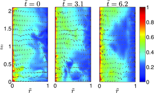
Figure 1: (color online) Three contour plots of the instantaneous angular velocity field $\omega$ for $Re_{s}=8.10\cdot 10^{3}$, $Ro^{-1}=1.22$, separated by $3.1$ nondimensional time units. Arrows represent the underlying axial and radial velocities. The first snapshot shows the initial field, and in the other two snapshots (at $\tilde{t}=3.1$ and $\tilde{t}=6.2$) reversals of the Taylor rolls can be seen: The radial velocity in the gap at mid-height ($\tilde{z}\approx 1.1$) changes from inwards in the first snapshot, to outwards in the second, and back again to inwards in the last.

To quantify these reversals, we define the quasi-Nusselt number eck07b $Nu_{\omega}(r,t)$ as $Nu_{\omega}(r,t)=r^{3}(\langle u_{r}\omega\rangle_{\theta,z}-\nu\partial_{r}\langle\omega\rangle_{\theta,z})/T_{pa}$, where $T_{pa}$ is the torque required to drive the system in the purely azimuthal and laminar case. $Nu_{\omega}(r,z)$ represents the transport of angular velocity. For a purely azimuthal flow with no turbulence, $Nu_{\omega}=1$, so $Nu_{\omega}-1$ represents the additional transport of angular velocity due to turbulence.

Figure 2a shows a time series of the axially averaged $Nu_{\omega}-1$ at the mid-radius $\tilde{r}=0.5$, for $Re_{s}=8.10\cdot 10^{3}$ and three values of the Coriolis force. $Nu_{\omega}-1$ can be seen to oscillate between large positive and large negative values, with an average $\approx 0$, i.e. no net turbulent transport. The period of oscillation depends on $Ro^{-1}$. Fig. 2c shows long time series for $Ro^{-1}=1.22$. For large enough times, the oscillations damp out and the flow becomes purely azimuthal and laminar, $Nu_{\omega}=1$. Fig. 2b shows $Nu_{\omega}-1$ for three values of $Re_{s}$ and $Ro^{-1}=1.22$. Similar oscillations in $Nu_{\omega}-1$ can be seen, but in this case the period weakly depends on $Re_{s}$.

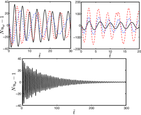
Figure 2: (a): Time series of $Nu_{\omega}-1$ at mid-gap for $Re_{s}=8.10\cdot 10^{3}$ and three values of $Ro^{-1}$, $Ro^{-1}=0.83$, (blue dash-dot line, Rayleigh-stability line), $Ro^{-1}=1.22$, (quasi-Keplerian, i.e. stable, black line) and $Ro^{-1}=2.50$ (even more stable, red dashed line), (b): Time series of $Nu_{\omega}(t)-1$ for $Ro^{-1}=1.22$ and three values of $Re_{s}$ (black line: $Re_{s}=8.10\cdot 10^{3}$, blue dashed line: $Re_{s}=2.52\cdot 10^{4}$, and red dash-dot line: $Re_{s}=8.10\cdot 10^{4}$), (c): longer time series of (a) for $Ro^{-1}=1.22$. On all figures (a), (b), (c) large oscillations of $Nu_{\omega}-1$ from positive to negative can be seen, which, when averaged, show that there is no net turbulent transport of angular velocity. For large enough time, the fluctuations decay and $Nu_{\omega}-1$ drops to zero.

Figure 3 shows the axially averaged $Nu_{\omega}-1$ but now measured directly at the inner cylinder (probing the inner boundary layer (BL)), for different values of $Ro^{-1}$ and $Re_{s}$. Unlike the previous mid gap case, no oscillations can be seen, reflecting that the oscillations only occur in the bulk of the flow, where the Taylor vortices are, but that the BLs are unaffected. Of course, the decay towards the purely azimuthal, laminar state $Nu_{\omega}=1$ is also observed in the BLs (Fig 3a,b), independent of $Ro^{-1}$ and $Re_{s}$.

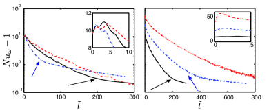
Figure 3: (a): semi-log time series of $Nu_{\omega}-1$ at the inner cylinder ($\tilde{r}=0$, $z$-averaged) for $Re_{s}=8.10\cdot 10^{3}$ and three values of $Ro^{-1}$, namely $Ro^{-1}=0.83$, (Rayleigh-stability line, blue dash-dot line), $Ro^{-1}=1.22$ (quasi-Keplerian, black line), and $Ro^{-1}=2.50$ (red dashed line). (b): semi-log time series of $Nu_{\omega}-1$ at the inner cylinder for $Ro^{-1}=1.22$ and three values of $Re_{s}$ (black line: $Re_{s}=8.10\cdot 10^{3}$, blue dashed line: $Re_{s}=2.52\cdot 10^{4}$, and red dash-dot line: $Re_{s}=8.10\cdot 10^{4}$). Two decay modes can be seen in this figure, with the crossovers marked with arrows. In both (a), (b), fluctuations are absent, unlike at the mid-gap, but $Nu_{\omega}-1$ decays. For large enough time, $Nu_{\omega}-1$ drops to zero, taking more time to do so for higher $Re_{s}$ or smaller $Ro^{-1}$. Zoom-ins of the first few large eddy turnover times are shown as insets (linear scale) for both figures. Transients, corresponding to an increase of $Nu_{\omega}$ can be seen during the initial stages.

Finally, we quantify the decay of turbulence. To do so, we define the turbulent kinetic energy substitute of the flow as $K(t)=\frac{1}{2}(u_{r}^{2}+u_{z}^{2})_{r,z,\theta}$. Note that this is not the full turbulent energy, as for that also fluctuations in $u_{\theta}$ contribute, but, by definition, $K$ has the nice property to be zero in the purely azimuthal state. Fig. 4a shows the decay of $K$ for $Re_{s}=8.10\cdot 10^{3}$ and three values of $Ro^{-1}$, while fig 4b shows the decay for $Ro^{-1}=1.22$ and three values of $Re_{s}$. In the simulations, $K(\tilde{t})$ shows short time scale fluctuations, similar to that of $Nu_{\omega}$ in the mid-gap, so for clarity, only the peak of $K(\tilde{t})$ in every cycle is represented.

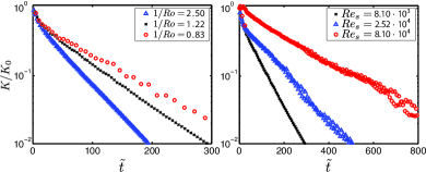
Figure 4: (a): Time series of $K(\tilde{t})/K_{0}$ for $Re_{s}=8.10\cdot 10^{3}$ and three values of $Ro^{-1}$, $Ro^{-1}=0.83$, (Rayleigh-stability line), $Ro^{-1}=1.22$, (quasi-Keplerian) and $Ro^{-1}=2.50$. (b): Time series of $K/K_{0}$ for $Ro^{-1}=1.22$ and three values of $Re_{s}$. After the initial transient, an exponential decay of the turbulent kinetic energy can be seen, even at the largest Reynolds numbers.

As expected from the previous results on $Nu_{\omega}(\tilde{t})$, $K(\tilde{t})$ decays to zero when given enough time. The only mechanism for energy dissipation is viscosity, so it is not surprising that the decay time is proportional to the energy content, thus leading to an approximately exponential decay, $K(\tilde{t})=K_{0}\exp(-\tilde{t}/\tilde{\tau})$ where $\tilde{\tau}$ is the characteristic (dimensionless) decay time, and $K_{0}=K(\tilde{t}=0)$. Fits to the data in fig. 4b were performed to obtain estimates for the dependence $\tilde{\tau}(Re_{s})$, which is shown in fig. 5a. The absolute value of $\tilde{\tau}$ is large (around $70$ large eddy turnover times for $Re_{s}\sim 10^{4}$ and $Ro^{-1}=1.22$) and in the range studied shows a power-law

$$\tilde{\tau}\sim\sqrt{Re_{s}}.$$ (2)

This scaling can be understood from realizing that the decay of the turbulence is first dominated by the energy dissipation rate $\epsilon_{BL}$ in the BLs, which scales as gro00 $\epsilon_{BL}\sim\nu^{3}d^{-4}Re_{s}^{5/2}$. This immediately implies the scaling relation (2) for the typical decay time $\tau=\tilde{\tau}d/U\sim U^{2}/\epsilon_{BL}$. Only for very large times or for very small Reynolds numbers from the very beginning, i.e., when the thickness of the BLs is comparable to the gap thickness $d$ and the Taylor rolls have died out or are absent, one has $\epsilon_{BL}\sim\nu^{3}d^{-4}Re_{s}^{2}$ (cf. ref. gro01 ) and thus $\tau\sim Re_{s}$. This second regime can be seen in figs. 3b and 5b.

We highlight that even though $K(\tilde{t})$ decays, the total energy of the system increases, as it absorbs more energy through the boundaries than it dissipates viscidly. This can be seen in fig.  5b, displaying a time series of the non-dimensionalized energy input into the system $\dot{E}=(T_{i}\omega_{i}+T_{o}\omega_{o})/(\rho\Omega\epsilon_{pa})$, where $T_{i,o}$ is the torque applied at the inner (outer) cylinder, $\rho$ and $\Omega$ are the fluid density and volume, respectively, and $\epsilon_{pa}$ is the viscous dissipation in the purely azimuthal and laminar state, and a time series of the non-dimensionalized energy dissipation rate inside the system, $\tilde{\epsilon}_{\nu}=\frac{1}{2}\nu\langle[\partial_{i}u_{j}+\partial_{j}u_{i}]^{2}\rangle_{\Omega}/\epsilon_{pa}$. When transitioning from turbulence to the purely azimuthal $u_{\theta}(r)$-profile, the system absorbs energy, while at the same time the initial turbulence decays. The purely azimuthal $u_{\theta}(r)$-profile has more energy than its turbulent counterpart. Indeed, this is the reason for the Rayleigh instability, now supressed by the Coriolis force.

Again, two time scales for the decay can be seen in the inset of fig 5b. After the initial transient, turbulence in the bulk decays fast, due to the efficient angular momentum transport by the Taylor rolls. After about 200-300 large eddy turnover times this decay mechanism is exhausted as then the (turbulent) Taylor rolls in the bulk are so weak that they can no longer transport angular momentum. Then a second decay mechanism takes over, whose onset is marked by an arrow in the inset of fig 5b. In this regime, characterized by purely viscous dissipation $\sim\nu^{3}L^{-4}Re_{s}^{2}$ in the whole gap, the profile $u_{\theta}(r)$ returns to the azimuthal and laminar one and $Nu_{\omega}$ thus to $1$. It is important to note that $Nu_{\omega}$ must return to $1$, as in the statistically stationary state, $Nu_{\omega}$ has to be independent of $r$.

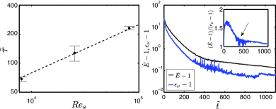
Figure 5: (a) log-log plot of the turbulence decay time $\tilde{\tau}$ vs $Re_{s}$ for $Ro^{-1}=1.22$ (quasi-Keplerian) and the three values of $Re_{s}$ simulated. The power law $\tilde{\tau}=0.79\sqrt{Re_{s}}$ fits the data points. (b): Semi-logarithmic plot of the time series of both the energy input through the boundaries $\dot{E}-1$ and the viscid dissipation of energy in the system $\tilde{\epsilon}_{\nu}-1$ for $Re_{s}=2.49\cdot 10^{4}$ and $Ro^{-1}=1.22$. The laminar dissipation, i.e. $1$ with the non-dimensionalization chosen, is subtracted from both variables. An inset with the ratio between both energies is shown. The arrow marks the transition between the two decay mechanisms. For quite a long time, the system still absorbs more energy than it dissipates; equilibrium is reached only for $\tilde{t}$ of order beyond $1000$, due to the small decay rate.

In summary, consistent with what had been found in the experiments of Ji et al.ji06 , no turbulence, and therefore, no turbulent transport of angular momentum can be seen in the Rayleigh-stable regime for the control parameter range studied once the effect of axial boundaries is mitigated. An initially turbulent state is stabilized by the corotation of the outer cylinder and the transport of angular momentum in the bulk ceases; the turbulence decays in all our simulations, for $Re_{s}$ up to $8.10\cdot 10^{4}$.

We point out, however, that even though the system is stable, the decay times for turbulence are long, ranging between hundreds and thousands of large eddy turnover times. If one extrapolates the scaling relation (2) to shear Reynolds numbers attainable in cold accretion disks, which are of the order $10^{14}$, decay times for the turbulence become very large, and the system might not have time to stabilize before enough angular momentum is transported and the disk collapses into a planetary system. It is also unclear whether the extreme values of $\eta$ present in astrophysical accretion disks will have an effect on the decay times. The Rossby number has a strong $\eta$-dependence, and for $\eta\to 0$ it diverges. Also, other types of mechanisms might dominate the angular momentum transport in cold accretion disks, like subcritical baroclinic instabilities which lead to turbulence wit74 ; kla03 or transport associated to self-gravity pac81 . We refer the reader to the review by Armitage arm11 for a more detailed discussion.

In conclusion, in our TC simulations without end-plates, in the parameter range studied up to shear Reynolds numbers of $10^{5}$, the flow was seen to not only remain laminar in the presence of small perturbations, but when starting from an initially turbulent state we can see that the turbulence decays and the system returns to its laminar state. All of this happens while the system absorbs energy. Therefore, we can attribute the turbulence and increased angular momentum transport found in some of the experiments dub05 ; pao11 and numerical simulations avi12 which probe the linearly stable regime of TC, to effects of the end-plate confinement.

Acknowledgments: We would like to thank C. Sun for various stimulating discussions. We acknowledge an ERC Advanced Grant and the PRACE resource Curie, based in France at GENCI/CEA.

References

- (1) H. Ji and S. A. Balbus, “Angular momentum transport in astrophysics and in the lab,” Phys. Today 66, 27–33 (Aug 2013).
- (2) P. J. Armitage, “Dynamics of protoplanetary disks,” Ann. Rev. Astron. Astrophys. 49 (2011).
- (3) N. I. Shakura and R. A. Sunyaev, “Black holes in binary systems. observational appearance..” Astron. & Astrophys 24, 337–355 (1973).
- (4) E. P. Velikhov, “Stability of an ideally conducting liquid flowing between rotating cylinders in a magnetic field,” Zhur. Eksptl’. i Teoret. Fiz. 36 (1959).
- (5) S. A. Balbus and J. Hawley, “A powerful local shear instability in weakly magnetized disks,” Astrophys. J. 376 (1991).
- (6) C. F. Gammie, “Layered accretion in T-Tauri disks,” Astrophys. J. 457 (1996).
- (7) L. N. Trefethen, A. E. Trefethen, S. C. Reddy, and T. A. Driscol, “Hydrodynamic stability without eigenvalues,” Science 261, 578–584 (1993).
- (8) S. Grossmann, “The onset of shear flow turbulence,” Rev. Mod. Phys. 72, 603–618 (2000).
- (9) D. Richard, Instabilités Hydrodynamiques dans les Ecoulements en Rotation Différentielle, Ph.D. thesis, Univ. Paris 7 (2001).
- (10) B. Dubrulle, O. Dauchot, F. Daviaud, P. Y. Longaretti, D. Richard, and J. P. Zahn, “Stability and turbulent transport in Taylor–Couette flow from analysis of experimental data,” Phys. Fluids 17, 095103 (2005).
- (11) H. Ji, M. Burin, E. Schartman, and J. Goodman, “Hydrodynamic turbulence cannot transport angular momentum effectively in astrophysical disks,” Nature 444, 343–346 (2006).
- (12) D. P. M. van Gils, S. G. Huisman, G. W. Bruggert, C. Sun, and D. Lohse, “Torque scaling in turbulent Taylor-Couette flow with co- and counter-rotating cylinders,” Phys. Rev. Lett. 106, 024502 (2011).
- (13) D. P. M. van Gils, S. G. Huisman, S. Grossmann, C. Sun, and D. Lohse, “Optimal Taylor-Couette turbulence,” J. Fluid Mech. 706, 118–149 (2012).
- (14) M. S. Paoletti and D. P. Lathrop, “Angular momentum transport in turbulent flow between independently rotating cylinders,” Phys. Rev. Lett. 106, 024501 (2011).
- (15) M. S. Paoletti, D. P. M. van Gils, B. Dubrulle, C. Sun, D. Lohse, and D. P. Lathrop, “Angular momentum transport and turbulence in laboratory models of keplerian flows,” Astron. & Astrophys 547, A64 (2012).
- (16) M. Avila, “Stability and angular-momentum transport of fluid flows between corotating cylinders,” Phys. Rev. Lett. 108, 124501 (2013).
- (17) G. Lesur and P. Y. Longaretti, “On the relevance of subcritical hydrodynamic turbulence to accretion disk transport,” Astron. & Astrophys 444, 25–44 (2005).
- (18) R. Verzicco and P. Orlandi, “A finite-difference scheme for three-dimensional incompressible flow in cylindrical coordinates,” J. Comput. Phys. 123, 402–413 (1996).
- (19) R. Ostilla, R. J. A. M. Stevens, S. Grossmann, R. Verzicco, and D. Lohse, “Optimal Taylor-Couette flow: direct numerical simulations,” J. Fluid Mech. 719, 14–46 (2013).
- (20) R. Ostilla, E. P. van der Poel, R. Verzicco, S. Grossmann, and D. Lohse, “Boundary layer dynamics at the transition between the classical and the ultimate regime of Taylor-Couette flow,” Phys. Fluids x, y (2014).
- (21) H. Brauckmann and B. Eckhardt, “Direct Numerical Simulations of Local and Global Torque in Taylor-Couette Flow up to Re=30.000,” J. Fluid Mech. 718, 398–427 (2013).
- (22) In the astrophysical context, e.g. ref. dub05 , often an extra factor is used in this definition.
- (23) G. I. Taylor, “Motion of solids in fluids when the flow is not irrotational,” Proc. R. Soc. Lond. A 93, 92–113 (1917).
- (24) J. Proudman, “On the motion of solids in a liquid possessing vorticity,” Proc. R. Soc. Lond. A 92, 408–424 (1916).
- (25) S. Chandrasekhar, Hydrodynamic and Hydromagnetic Stability (Dover, New York, 1981).
- (26) B. Eckhardt, S. Grossmann, and D. Lohse, “Torque scaling in turbulent taylor-couette flow between independently rotating cylinders,” J. Fluid Mech. 581, 221–250 (2007).
- (27) S. Grossmann and D. Lohse, “Scaling in thermal convection: A unifying view,” J. Fluid. Mech. 407, 27–56 (2000).
- (28) S. Grossmann and D. Lohse, “Thermal convection for large Prandtl number,” Phys. Rev. Lett. 86, 3316–3319 (2001).
- (29) I.e., ignoring possible crossovers to an ultimate regime in which the energy dissipation rate may be dominated by the bulk dissipation gro00 ; gro11 . In that regime would become independent on .
- (30) E. M. Withjack and C. F. Chen, “An experimental study of couette instability of stratified fluids,” J. Fluid Mech. 66, 725–737 (1974).
- (31) H.H. Klahr and P. Bodenheimer, “Turbulence in accretion disks: Vorticity generation and angular momentum transport via the global baroclinic instability,” The Astrophysical Journal 508, 869 (2003).
- (32) B. Paczynski and G. Bisnovatyi-Kogan, “A model of a thin accretion disk around a black hole,” Acta Astronomica 31 (1981).
- (33) S. Grossmann and D. Lohse, “Multiple scaling in the ultimate regime of thermal convection,” Phys. Fluids 23, 045108 (2011).