MAGNA: Maximizing Accuracy in Global Network Alignment

Vikram Saraph and Tijana Milenković^∗
Department of Computer Science and Engineering
University of Notre Dame, Notre Dame, IN 46556, USA
^∗Corresponding Author (E-mail: tmilenko@nd.edu)

Summary

Biological network alignment aims to identify similar regions between networks of different species. Existing methods compute node “similarities” to rapidly identify from possible alignments the “high-scoring” alignments with respect to the overall node similarity. However, the accuracy of the alignments is then evaluated with some other measure that is different than the node similarity used to construct the alignments. Typically, one measures the amount of conserved edges. Thus, the existing methods align similar nodes between networks hoping to conserve many edges (after the alignment is constructed!).

Instead, we introduce MAGNA to directly “optimize” edge conservation while the alignment is constructed. MAGNA uses a genetic algorithm and our novel function for “crossover” of two “parent” alignments into a superior “child” alignment to simulate a “population” of alignments that “evolves” over time; the “fittest” alignments survive and proceed to the next “generation”, until the alignment accuracy cannot be optimized further. While we optimize our new and superior measure of the amount of conserved edges, MAGNA can optimize any alignment accuracy measure. In systematic evaluations against existing state-of-the-art methods (IsoRank, MI-GRAAL, and GHOST), MAGNA improves alignment accuracy of all methods.

1 Introduction

1.1 Motivation and background

Genomic sequence alignment has led to breakthroughs in our understanding of how cells work. It identifies regions of similarity between sequences of individual genes that are a likely consequence of evolutionary relationships between the sequences. However, genes, i.e., their protein products, do not act alone but instead interact with each other to carry out cellular processes. And this is exactly what protein-protein interaction (PPI) networks model. (While we focus on PPI networks, our ideas are applicable to any network type.) Then, network alignment (NA) can be used to find regions of similarities between PPI networks of different species that are a likely consequence of evolutionary relationships between the networks. Unlike sequence alignment that ignores genes’ interconnectivities, NA allows for studying complex cellular events that are a consequence of the collective behavior of the genes’ protein products. As such, NA is promising to further our biological understanding [1].

As recent biotechnological advances continue to yield large amounts of PPI data [2], alignment of PPI networks of different species continues to gain importance [1]. This is because NA could guide the transfer of biological knowledge across species between conserved (aligned) network regions [1]. This is important, since many proteins remain functionally uncharacterized even for well studied species [3]. Traditionally, the across-species transfer of biological knowledge has relied on sequence alignment. However, since PPI networks and sequences can capture complementary functional slices of the cell, implying that PPI networks can uncover function that cannot be uncovered from sequences by current methods, restricting alignment to sequences may limit the knowledge transfer [4].

Unfortunately, the mathematics of complexity theory dictates that exact network (or graph) comparison is computationally intractable. The underlying problem is that of subgraph isomorphism, which asks whether one graph (the source) appears as an exact subgraph of another graph (the target). Answering this is NP-complete [5]. Furthermore, simply answering the subgraph isomorphism problem is not enough when comparing PPI networks, since one PPI network is rarely an exact subnetwork of another due to biological variation [6]. It is much more desirable to answer how similar two networks are and in what regions they share similarity. NA can be used for this purpose.

NA is a less restrictive problem than that of subgraph isomorphism, as it seeks to “fit” the source into the target in the “best possible way” even if the source is not an exact subgraph of the target. An alignment is a mapping between nodes of the source and nodes of the target that is expected to conserve as much structure (or topology) as possible between the two networks. (Note that methods exist that can align more than two networks [7, 8], but we focus on pairwise NA.) Since NA is computationally hard, heuristic methods must be sought.

NA can be local (LNA) or global (GNA). Initial solutions for NA have aimed to match local network regions [9, 10, 11, 12, 13, 14, 15]. That is, in LNA, subnetworks, rather than the entire networks, are aligned. However, aligned regions can overlap, leading to “ambiguous” many-to-many node mappings. Thus, GNA solutions have been proposed [16, 8, 17, 18, 7, 6, 19, 20, 21, 22, 23, 24]. In contrast to LNA, GNA compares entire networks, typically by aligning every node in the source to exactly one unique node in the target. We focus on GNA, but our ideas are also applicable to LNA.

Traditionally, GNA has relied on biological information external to network topology, e.g., sequence similarity [1]. To extract the most from each source of biological information, it would be good to know how much of new biological knowledge can be uncovered solely from network topology before integrating it with other sources of biological information [6, 19, 20, 21, 24]. Only after methods for topological GNA are developed that result in alignments of good topological and biological quality, it would be beneficial to integrate them with other biological data sources to further improve the quality. Thus, we focus on topological GNA, but additional biological data can easily be added.

Existing GNA methods, of which the more prominent ones (and which we consider in our study) are outlined below, typically use a two-step approach: (1) score the “similarity” of pairs of nodes from different networks, and (2) feed these scores into an alignment strategy to identify “high-scoring” alignments from all possible alignments.

IsoRank [16] scores nodes from two networks by a PageRank-based spectral graph theoretic principle: two nodes are a good match if their neighbors are good matches. After these topological scores are computed, biological scores can be added to get final node scores. An alignment is then constructed by greedily matching the high-scoring node pairs. IsoRank has evolved into IsoRankN to allow for multiple GNA [7] and many-to-many node mapping, but this is out of the scope of our study.

The GRAAL family of algorithms [6, 19, 25, 20], developed in parallel with the IsoRank family, use graphlet (or small induced subgraph) counts to compute mathematically rigorous topological node similarity scores [26, 27, 28]. Intuitively, two nodes are a good match if their extended network neighborhoods are “topologically similar” with respect to the graphlet counts. Also, MI-GRAAL [20], the latest of the family members, can automatically add other (biological) node similarity scores into final scores. It is the alignment strategies of the GRAAL family members that are different. MI-GRAAL combines alignment strategies of the other members, thus outperforming each of them [20].

More recent GHOST [21] uses “spectral signatures” to score node pairs topologically while also allowing for inclusion of biological node scores. Similar to MI-GRAAL, GHOST’s alignment strategy is also seed-and-extend, except that GHOST solves a quadratic assignment problem, while MI-GRAAL solves a linear assignment problem.

1.2 Our contribution

Recall that the existing GNA methods construct alignments by scoring all node pairs with respect to the nodes’ similarities and by rapidly identifying “high-scoring” alignments from all possible alignments. Here, “high-scoring” alignments are typically those that “maximize” (greedily or optimally) the node similarity score totaled over all mapped nodes [16, 6, 19, 20, 21]. However, the accuracy (or quality) of the alignments is then evaluated with respect to some other measure of an inexact fit of two networks, which is different than the node scoring function that is used to construct the alignments in the first place. Typically, one measures the amount of conserved edges (see below) [20, 21]. (One also evaluates the alignments biologically with respect to functional knowledge.) Thus, the existing methods align “similar” nodes between networks with the goal (or hope!) of conserving as many edges as possible under the alignment (after the alignment is constructed!). Instead, we introduce MAGNA, a new framework for directly “maximizing” (or “optimizing”) accuracy in GNA with respect to the amount of conserved edges while the alignment is being constructed, which is our first contribution.

Optimizing the amount of conserved edges would require finding a global optimum over the search space consisting of all possible node mappings. Due to the large size of the space, exhaustive search is computationally intractable. But, approximate techniques exist with solutions very close to optimal, such as genetic algorithms [29]. Hence, we adapt the idea of genetic algorithms to the problem of GNA to develop MAGNA as a conceptually novel GNA framework. This is our second contribution, since to our knowledge, genetic algorithms have not been used for PPI GNA thus far. MAGNA simulates a “population” of alignments that “evolves” over time (the initial population can consist of random alignments or of alignments produced by the existing methods). Then, the “fittest” candidates (those that conserve the most edges) survive and proceed to the next generation. This is repeated until the algorithm converges, i.e., until the amount of conserved edges cannot be optimized further.

Much of what defines any genetic algorithm is the crossover function, which “combines” two candidates (i.e., alignments) into a new one. And since genetic algorithms have not been used for GNA thus far, we had to devise a novel (and to our knowledge, the first ever) function for crossover of two parent alignments into a child alignment that reflects (ideally the best of) each parent. The alignment crossover function is the third and a major contribution of our study, because it allows MAGNA not only to combine alignments produced by any existing method to improve them but also to produce its own new superior alignments.

It is not obvious how to measure the quality of an alignment [19], i.e., which measure to optimize as the “fitness” function within the genetic algorithm. Clearly, a good alignment should maximize the amount of conserved edges. Different measures have been proposed to quantify this, all of which are heuristics and thus correctly reflect the actual alignment quality in some cases but fail to do so in other cases. Thus, as our fourth contribution, we introduce a new and superior alignment quality measure that takes the best from each existing measure. While we optimize with MAGNA this new measure as well as the existing measures of the amount of conserved edges, importantly, MAGNA can optimize any measure of alignment quality, topological or biological, which is another of our contributions.

We evaluate MAGNA against IsoRank, MI-GRAAL, and GHOST by aligning a high-confidence yeast PPI network with its noisy counterparts, where the true node mapping is known. This popular evaluation test [6, 20, 21] allows for a systematic method comparison. MAGNA improves alignment quality of all of the existing methods.

2 Methods

2.1 Alignment crossover function

In this section, we provide the mathematical rigor necessary to define our novel “crossover function”, which is at the heart of MAGNA. (The description of MAGNA is given in Section 2.2.) The crossover function should take two “parent” alignments and produce a “child” alignment that is intended to reflect (ideally the best of) both parents.

Let $G_{1}(V_{1},E_{1})$ and $G_{2}(V_{2},E_{2})$ be two networks with $V_{i}$ and $E_{i}$ as the sets of nodes and edges, respectively. Let $m=|V_{1}|$ and $n=|V_{2}|$. Without loss of generality, suppose $|V_{1}|\leq|V_{2}|$. An alignment of $G_{1}$ to $G_{2}$ is a total injective function $f:V_{1}\rightarrow V_{2}$. That is, every element of $V_{1}$ is matched uniquely with an element of $V_{2}$. If $|V_{1}|=|V_{2}|$, when $f$ is an injective function, then in fact $f$ is a bijection.

Let $V_{1}=\{x_{1},\ldots,x_{m}\}$ and $V_{2}=\{y_{1},\ldots,y_{n}\}$. Let $[n]=\{1,\ldots,n\}$ be the set of natural numbers from 1 to $n$. A permutation is a bijection $\sigma:[n]\rightarrow[n]$. Then, with the assumption that $m=n$, and given this fixed number labeling of nodes as above, we can represent any alignment $f$ with a corresponding permutation $\sigma$ that maps node labels to node labels. Even though it is rare that $|V_{1}|=|V_{2}|$, we can easily force this condition to be true by adding dummy, zero-degree nodes $z_{i}$ to $V_{1}$, as follows: $\bar{V_{1}}=V_{1}\cup\{z_{m+1},\ldots,z_{n}\}$. Thus, from now on, we will simply assume that $|V_{1}|=|V_{2}|$, without explicitly referring to $\bar{V_{1}}$. Therefore, any alignment can be represented as a permutation, and for the remainder of this section, we use “permutation” and “alignment” interchangeably. This representation is critical to our crossover function.

Let $S_{n}$ denote the set of all permutations. Notice that $|S_{n}|=n!$, which is large. In theory, to find an alignment of maximum quality (with respect to a given criterion), we could “simply” enumerate all permutations and evaluate the quality of each one. However, this is impractical due to the large size of $S_{n}$, so we require a clever search heuristic. We design such a heuristic as follows. First, we create a graph with $S_{n}$ as the set of nodes in which two permutations (alignments) are connected by an edge if the alignments are “adjacent” (see below). Second, since intuitively the alignment quality is continuous in alignment “adjacency” (in the sense that two “adjacent” alignments should be of similar quality, or in other words, a small perturbation of an alignment should not greatly affect its quality), we exploit the topology of this graph to define a function for crossover of two alignments. Namely, we define the child alignment as the alignment that is “in the middle” between two given parent alignments in this graph. Formal details are as follows.

Given two permutations $\sigma$ and $\tau$, we define what it means for $\sigma$ and $\tau$ to be adjacent. A transposition of a permutation is a new permutation that fixes every element of the original permutation, except two elements, which are swapped. Then, two permutations are adjacent if they differ by a transposition; that is, $\sigma$ and $\tau$ are adjacent if there is a transposition $\rho$ such that $\sigma=\rho\circ\tau$. We create graph $\Gamma_{n}$ with the set of nodes $S_{n}$ and the set of edges $E_{n}$, where an edge between $\sigma$ and $\tau$ is in $E_{n}$ if and only if $\sigma$ and $\tau$ are adjacent. Then, we define $\sigma\otimes\tau$, the crossover of any two permutations $\sigma$ and $\tau$ from $S_{n}$, as a permutation which is the midpoint on a shortest path from $\sigma$ to $\tau$ in $\Gamma_{n}$. This definition captures what we desire from a crossover function. More precisely, it can be shown that for randomly selected permutations $\sigma$ and $\tau$, $|\sigma\cap(\sigma\otimes\tau)|/n\rightarrow 1/2$ and $|\tau\cap(\sigma\otimes\tau)|/n\rightarrow 1/2$ as $n\rightarrow\infty$. That is, $\sigma\otimes\tau$ is expected to share approximately half of its aligned pairs with $\sigma$, and likewise with $\tau$. A proof of the above statement relies on the fact that the expected number of cycles in a permutation is $\Theta(\log(n))$. We leave out further discussion on this, as it would require more basics of abstract algebra, which is beyond the scope of this paper; see [30, 31] for details.

2.2 MAGNA: genetic algorithm-based GNA framework

A genetic algorithm mimics the evolutionary process, guided by the “survival of the fittest” principle [32]. It begins with an initial “population” of a given number of “members”. Members of a population “crossover” with one another to produce new members. The “child” resulting from a crossover should resemble both of its “parents”. Crossing over different pairs of members at a given generation yields new members, which comprise the new “generation” of members. The probability of a member being given a chance to crossover with another member is determined by its “fitness,” so that fitter members are more likely to crossover. To prevent the size of the population to grow without bound, the size is kept constant across all generations, with only the fittest members surviving from one generation to the next. To ensure that the maximum fitness of the population is nondecreasing, with each generation, a designated “elite” class of the fittest members is automatically passed to the next generation. As the algorithm progresses, newer generations are produced, with fitness (hopefully) increasing, until a stopping criterion is reached. To specify a genetic algorithm, we need to specify all of the above parameters.

In MAGNA, members of a population are alignments. We use different types of initial populations: 1) all random alignments, 2) random alignments mixed with an IsoRank’s alignment, 3) random alignments mixed with a MI-GRAAL’s alignment, and 4) random alignments mixed with a GHOST’s alignment. Since we focus on topological network alignments (Section 1.1), we produce all alignments by using only topological information in the existing methods’ node scoring function. For each type of initial population, we test populations of different sizes: 200, 500, 1,000, 2,500, 5,000, 10,000, and 15,000. (It is because the population sizes are large that we cannot form an initial population consisting only of alignments produced by an existing method, due to large computational complexity of the existing methods. Instead, we use in the initial population an existing alignment and fill the remaining part of the population with random alignments.) The mathematical machinery from Section 2.1 gives us a suitable crossover function for producing a child alignment that resembles both of its parent alignments. Our fitness function is the measure of alignment quality we choose to optimize; in our case, it is edge correctness (EC), induced conserved structure (ICS), or symmetric substructure score (S³) (Section 2.3), but it can be any measure. In every generation, we keep the best half of the population from the previous generation, and we fill the remaining half of the population with alignments produced by crossovers. We select pairs of alignments to be crossed as follows. At a given generation of population size $p$, we have ${p\choose 2}$ crossover possibilities. This is too large a number to consider all of them. Thus, to select crossover pairs, we use roulette wheel selection, which is a commonly adopted selection strategy for genetic algorithms [32]. Roulette wheel selection chooses members with probability in linear proportion to the members’ fitness. We let MAGNA run for many generations. We vary the number of generations from 0 to 2,000 in increments of 200. The fittest alignment from the last generation is reported as the final alignment. We describe MAGNA in the pseudocode (Supplementary Algorithm S1). We provide MAGNA’s implementation upon request.

Our implementation of the alignment crossover function takes $O(|V|)$ time. MAGNA’s bottleneck, though, tends to be the computation of alignment quality $F$. If the measure of $F$ is EC, ICS, or S³, then for a given alignment, it takes $O(|E|\log(|E|))$ time to compute $F$. Finally, sorting each generation of size $p$ takes $O(p\log(p))$ time, though this is typically negligible compared to the computation of $F$. If MAGNA is run for $N$ generations, this brings the overall time complexity of MAGNA to $O(N(p|V|+p|E|\log(|E|)+p\log(p)))$. Note that most of MAGNA is embarrassingly parallelizable, which can lead to a very high degree of speedup.

2.3 New alignment quality measure

To motivate our new measure of alignment quality, the symmetric substructure score (S³), we first present drawbacks of existing edge correctness (EC) and induced conserved structure (ICS) measures.

Let $G_{1}(V_{1},E_{1})$ and $G_{2}(V_{2},E_{2})$ be two networks, and let $f:V_{1}\rightarrow V_{2}$ be an alignment between them. If $X\subseteq V_{2}$, let $G_{2}[X]$ be the induced subnetwork of $G_{2}$ with node set $X$. Also, if $H$ is a subnetwork of $G_{2}$, let $E(H)$ be its edge set. Let $f(E_{1})=\{(f(u),f(v))\in E_{2}:(u,v)\in E_{1}\}$, and let $f(V_{1})=\{f(v)\in V_{2}:v\in V_{1}\}$.

EC of $f$ is the ratio of the number of edges conserved by $f$ to the number of edges in the source network: $\text{EC}(f)=\dfrac{|f(E_{1})|}{|E_{1}|}$ [6]. Because EC is defined with respect to the source but not the target network, it fails to penalize alignments mapping sparser network regions to denser ones (Fig. 1).

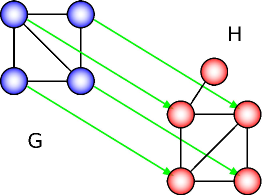
Figure 1: Illustration of our new S³ measure and its difference with EC and ICS. The illustrated alignment between nodes in network $G$ and nodes in network $H$ has an EC of $4/5=0.8$, an ICS of $4/5=0.8$, but an S³ of $4/6=0.67$. EC rewards for aligning four edges in $G$ to four edges in $H$ and penalizes for misaligning an edge in $G$ to a non-edge in $H$, but it fails to penalize for misaligning a non-edge in $G$ to an edge in $H$. Similarly, ICS rewards for aligning four edges in $G$ to four edges in $H$ and penalizes for misaligning an edge in $H$ (between the aligned nodes) to a non-edge in $G$, but it fails to penalize for misaligning an edge in $G$ to a non-edge in $H$. Like EC and ICS, S³ also rewards for aligning four edges in $G$ to four edges in $H$, but unlike EC or ICS, S³ penalizes for misaligning both an edge in $G$ to a non-edge in $H$ and a non-edge in $G$ to an edge in $H$.

ICS of $f$ is the ratio of the number of edges conserved by $f$ to the number of edges in the subnetwork of $G_{2}$ induced on the nodes in $G_{2}$ that are aligned to the nodes in $G_{1}$: $\text{ICS}(f)=\dfrac{|f(E_{1})|}{|E(G_{2}[f(V_{1})])|}$ [21]. Because ICS is defined with respect to the target but not the source network, it fails to penalize alignments mapping denser network regions to sparser ones (Fig. 1).

Therefore, we define S³ with respect to both the source network and the target network: $\text{S}^{3}(f)=\dfrac{|f(E_{1})|}{|E_{1}|+|E(G_{2}[f(V_{1})])|-|f(E_{1})|}$. The difference between EC, ICS, and S³ is the denominator. Intuitively, if $G_{1}$ and $G_{2}[f(V_{1})]$ are overlaid into a composite graph, then the denominator of S³ is the number of unique edges in this composite graph. Thus, S³ of an alignment is 100% if and only if $f$ is a perfect embedding. As such, S³ penalizes both alignments that map denser network regions to sparser ones and alignments that map sparser network regions to denser ones (Fig. 1).

3 Results and discussion

3.1 Validating MAGNA on networks with known node mapping

3.1.1 Data description

We aim to validate MAGNA by analyzing the largest connected component of the high-confidence yeast S. cerevisiae PPI network [33] with 1,004 proteins and 8,323 PPIs. We align this network with the same network augmented with lower-confidence PPIs from the same study [33]. We analyze different noise levels, by adding 0%, 5%, 10%, 15%, 20%, and 25% of lower-confidence PPIs; we add higher-scoring lower-confidence PPIs first. Since the networks being aligned are defined on the same set of nodes and differ only in the number of edges, we know the correct node mapping. An additional advantage of aligning these networks is that the original is an exact subgraph of each noisy network.

3.1.2 MAGNA parameters

MAGNA requires several parameters: the type of initial population, population size, maximum number of generations (i.e., iterations of the genetic algorithm), and optimization function (i.e., alignment quality measure) (Sections 2.2 and 2.3). We evaluate MAGNA comprehensively and systematically, by varying values of each parameter.

We use four different population types: random, IsoRank, MI-GRAAL, and GHOST. The random population aims to produce a high-quality alignment from scratch (by relying only on our new alignment crossover function), while the other three population types try to improve upon the existing methods. We test seven population sizes from 200 to 15,000. We vary the maximum number of generations up to 2000, in increments of 200. We optimize three alignment quality measures: EC, ICS, and S³. See Sections 2.2 and 2.3 for details.

Each combination of initial population type, population size, maximum number of generations, and optimization function results in one final (best) alignment. This comprehensive testing has resulted in the total of 5,544 final alignments.

The effect of the initial population type. Since we aim to compare MAGNA against IsoRank, MI-GRAAL, and GHOST (and also random alignments), we continue by considering all four initial population types and we discuss their effect on the alignment quality in more detail below.

The effect of population size. We find that, in general, larger population size is always preferred, independent of the initial population type, maximum number of generations, and optimization measure (Supplementary Section S1 and Supplementary Fig. S1). Henceforth, we continue with the largest population size of 15,000.

The effect of the maximum number of generations. We find that, in general, the larger the population size, the larger number of generations is preferred, which is $\sim$2,000 for random initial population, independent on the optimization measure, and $\sim$400-1,200 for IsoRank, MI-GRAAL, or GHOST initial population, depending on the optimization measure (Supplementary Section S1 and Supplementary Fig. S1). In general, GHOST initial population “converges” faster than MI-GRAAL and IsoRank populations. Because of the design of MAGNA, the alignment quality never drops from one generation to the following one. Thus, even with IsoRank, MI-GRAAL, and GHOST populations, the results are never worse at the 2,000^th generation compared to the 400-1,200^th generation. Thus, henceforth, we continue with the maximum number of generations of 2,000, since this helps for at least one population type without harming others. However, it is encouraging that some methods can converge very fast, indicating that MAGNA can produce high-quality alignments in short time.

The effect of the optimization measure. Since we aim to compare our new S³ measure with existing EC and ICS measures, we continue by considering all three and we discuss their effect on the alignment quality in more detail below.

3.1.3 MAGNA evaluation and comparison with existing methods

For each of the six noise levels, four initial population types (each of size 15,000), and three optimization measures, we obtain with MAGNA one final alignment, i.e., the best alignment (with respect to the given optimization measure) at the 2,000^th generation. In addition, we study the original alignments produced by the existing methods. Then, we compare these original alignments to those produced by MAGNA to see whether MAGNA improves the alignment quality of the existing alignments. Note that independent on which of the three alignment quality measures (EC, ICS, or S³) we optimize, the question remains on how to best evaluate the correctness of the resulting final alignment. Certainly, we could use any of the three alignment quality measures for this purpose. However, since the true node mapping is known when aligning the high-confidence yeast PPI network to its noisy counterparts, we can actually evaluate each method more fairly by counting the number of correctly aligned node pairs (or “node correctness”).

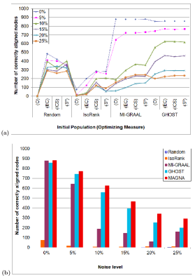
Figure 2: Correctness of alignments produced on noisy yeast networks (for noise levels in 0%-25% range), with respect to the number of correctly aligned node pairs. Panel (a) shows results for alignments produced by four existing algorithms (Random, IsoRank, MI-GRAAL, and GHOST) as well as by running MAGNA on populations containing the alignments produced by the existing algorithms. We use four different populations, corresponding to the four existing algorithms. For each population, we show results for an original alignment produced by the existing algorithm (O), as well as for MAGNA’s alignments produced when optimizing each of the following: EC, ICS, and $S^{3}$. All results are for population size of 15,000 and for 2,000 generations. Correctness of the alignments with respect to additional criteria, including EC, ICS, and S³, are shown in Supplementary Fig. S2 and S3. Panel (b) shows, for each noise level, comparison of results from panel (a) between MAGNA’s best alignment (over all initial population types and optimization measures) and the original alignments of the existing methods. (In most cases, original random alignments have scores close to 0 and are thus not visible.)

When we do this, we find that MAGNA improves all of the original alignments (i.e., all of the existing methods), across all levels of noise, and for each of the three optimization measures (Fig. 2). If we compute the “improvement” of MAGNA over an existing method as the ratio of MAGNA’s node correctness to the existing method’s node correctness, then MAGNA’s improvement is up to 2,588% upon IsoRank, up to 256% upon MI-GRAAL, and up to 118% upon GHOST, depending on the noise level and optimization measure. In general, the higher the noise level, the larger our improvements upon the existing methods (Fig. 2).

The effect of the initial population type. GHOST’s original alignments are overall slightly superior or comparable to MI-GRAAL’s original alignments, depending on the noise level and the optimization measure, both are superior to IsoRank’s original alignments, and all three are superior to random original alignments (Fig. 2). These results are consistent to those in the existing literature [6, 20, 21]. Thus, one might expect that MAGNA’s improved alignments of GHOST would be of better quality than MAGNA’s improved alignments of MI-GRAAL, that both would be of higher quality than MAGNA’s improved alignments of IsoRank, and that all three would be of higher quality than MAGNA’s improved alignments of random alignments. However, interestingly, we find that this is not always the case (Fig. 2). Actually, in many cases, there are surprising effects of the choice of the initial population type. For example, our improved alignments of MI-GRAAL are sometimes better than our improved alignments of GHOST. Or, even more interestingly, for larger noise levels, it is the random population that results in the best alignments; that is, we improve more when starting from completely random alignments than we do when starting from the original alignments of IsoRank, MI-GRAAL, or GHOST (Fig. 2). More precisely, when we measure, for each of the six noise levels, which initial population type results in the final alignment with the highest node correctness score over all four population types, we find that GHOST’s initial population is the best for three out of six noise levels (5%, 10%, and 15%), random initial population is the best for two noise levels (20% and 25%), and MI-GRAAL’s initial population is the best for the remaining noise level (0%).

The above results suggest that MAGNA is not only capable of improving alignments generated by the existing methods, but it is also capable of generating from completely random alignments its own new alignments that are superior, especially for the higher noise levels. Interesting implications are as follows. First, because current PPI networks are likely even noisier than those used in this section [34, 35], our results suggest that one might be able to improve upon the current best PPI network alignments (of different species, when the actual node mapping is unknown) simply by using MAGNA on completely random alignments of the PPI networks. Second, recall that random initial population converges the slowest of all populations, if at all. And recall that we stop MAGNA after 2,000 iterations, as all initial population types but random one converge even before that. Because of this, and because random population is superior for larger noise levels, it is possible that for such noise levels, the alignment quality could be improved even further by running MAGNA longer, as dictated by the available computing resources.

The effect of the optimization measure. No single optimization measure (out of EC, ICS, and S³) is always superior with respect to the node correctness as the alignment quality measure; the results depend on the choice of MAGNA’s parameters. Over all noise levels, random initial population prefers (in the sense that it results in the highest node correctness for) EC and S³ equally, IsoRank initial population prefers ICS, MI-GRAAL’s initial population prefers S³, and GHOST initial population prefers EC (Fig. 2). Hence, S³, as well as EC, seem to be preferred overall in this context. Over all population types, four of the six noise levels (5%, 10%, 15%, and 25%) prefer EC, one noise level (0%) prefers S³, and the remaining noise level (20%) prefers ICS. Hence, EC seems to be preferred overall in this context. We even further study the effect of the three optimization measures by computing Pearson correlation between the “node correctness” on one hand and EC, ICS, or S³ on the other, across all alignments from Fig. 2. A higher and more statistically significant correlation would indicate that the given optimization measure is capable of uncovering more correct alignments. The node correctness correlates the best and the most significantly with our new S³ measure, suggesting its superiority over the existing measures (Table 1).

measure	correlation	$p$-value
EC	0.7538	$3.9\times 10^{-19}$
ICS	0.8339	$2.7\times 10^{-26}$
S3	0.8980	$1.4\times 10^{-35}$

Table 1: Correlation between the node correctness and each of EC, ICS, and S³.

4 Concluding remarks

We present a conceptually novel framework for “optimizing” pairwise global network alignment with respect to any alignment quality measure, which outperforms the existing state-of-the-art methods. Given the tremendous amounts of biological network data that are being produced, network alignment will only continue to gain importance, as it can be used to transfer biological knowledge from well characterized species to poorly characterized ones between aligned network regions. Also, analogous to sequence alignment, network alignment can be used to infer species’ phylogeny based on similarities of their biological networks. Thus, it could lead to new discoveries about the principles of life, evolution, disease, and therapeutics.

References

- [1] Sharan R, Ideker T. Modeling cellular machinery through biological network comparison. Nature Biotechnology. 2006;24(4):427–433.
- [2] Breitkreutz BJ, Stark C, Reguly T, Boucher L, Breitkreutz A, Livstone M, et al. The BioGRID Interaction Database: 2008 update. Nucleic Acids Research. 2008;36:D637–D640.
- [3] Sharan R, Ulitsky I, Shamir R. Network-based prediction of protein function. Molecular Systems Biology. 2007;3(88):1–13.
- [4] Memisević V, Milenković T, Pržulj N. Complementarity of network and sequence information in homologous proteins. Journal of Integrative Bioinformatics. 2010;7(3):135.
- [5] Cook SA. The complexity of theorem-proving procedures. In: Proceedings of the 3rd Annual ACM Symposium on Theory of Computing; 1971. p. 151–158.
- [6] Kuchaiev O, Milenković T, Memišević V, Hayes W, Pržulj N. Topological network alignment uncovers biological function and phylogeny. Journal of the Royal Society Interface. 2010;7:1341–1354.
- [7] Liao C, Lu K, Baym M, Singh R, Berger B. IsoRankN: spectral methods for global alignment of multiple protein networks. Bioinformatics. 2009;25(12):i253–258.
- [8] Flannick J, Novak AF, Do CB, Srinivasan BS, Batzoglou S. Automatic Parameter Learning for Multiple Network Alignment. In: Research in Computational Molecular Biology (RECOMB); 2008. p. 214–231.
- [9] Kelley BP, Bingbing Y, Lewitter F, Sharan R, Stockwell BR, Ideker T. PathBLAST: a tool for alignment of protein interaction networks. Nucleic Acids Research. 2004;32:83–88.
- [10] Sharan R, Suthram S, Kelley RM, Kuhn T, McCuine S, Uetz P, et al. Conserved patterns of protein interaction in multiple species. Proceedings of the National Academy of Sciences. 2005;102(6):1974–1979.
- [11] Flannick J, Novak AF, Balaji SS, Harley HM, Batzglou S. Graemlin: General and robust alignment of multiple large interaction networks. Genome Research. 2006;16(9):1169–1181.
- [12] Koyuturk M, Kim Y, Topkara U, Subramaniam S, Szpankowski W, Grama A. Pairwise alignment of protein interaction networks. Journal of Computational Biology. 2006;13(2).
- [13] Berg J, Lassig M. Local graph alignment and motif search in biological networks. Proceedings of the National Academy of Sciences. 2004;101:14689–14694.
- [14] Liang Z, Xu M, Teng M, Niu L. NetAlign: a web-based tool for comparison of protein interaction networks. Bioinformatics. 2006;22(17):2175–2177.
- [15] Berg J, Lassig M. Cross-species analysis of biological networks by Bayesian alignment. Proceedings of the National Academy of Sciences. 2006;103(29):10967–10972.
- [16] Singh R, Xu J, Berger B. Pairwise Global Alignment of Protein Interaction Networks by Matching Neighborhood Topology. In: Research in Computational Molecular Biology (RECOMB). Springer; 2007. p. 16–31.
- [17] Singh R, Xu J, Berger B. Global Alignment of Multiple Protein Interaction Networks. Proceedings of Pacific Symposium on Biocomputing. 2008;p. 303–314.
- [18] Zaslavskiy M, Bach F, Vert JP. Global alignment of protein-protein interaction networks by graph matching methods. Bioinformatics. 2009;25(12):i259–i267.
- [19] Milenković T, Ng WL, Hayes W, Pržulj N. Optimal network alignment with graphlet degree vectors. Cancer Informatics. 2010;9:121–137.
- [20] Kuchaiev O, Pržulj N. Integrative Network Alignment Reveals Large Regions of Global Network Similarity in Yeast and Human. Bioinformatics. 2011;27(10):1390–1396.
- [21] Patro R, Kingsford C. Global network alignment using multiscale spectral signatures. Bioinformatics. 2012;28(23):3105–3114.
- [22] Narayanan A, Shi E, Rubinstein BIP. Link prediction by de-anonymization: How We Won the Kaggle Social Network Challenge. In: Proceedings of the 2011 International Joint Conference on Neural Networks (IJCNN). IEEE; 2011. p. 1825–1834.
- [23] Klau GW. A new graph-based method for pairwise global network alignment. BMC Bioinformatics. 2009;10(Suppl 1):S59.
- [24] Neyshabur B, Khadem A, Hashemifar S, Arab SS. NETAL: a new graph-based method for global alignment of protein–protein interaction networks. Bioinformatics. 2013;.
- [25] Memišević V, Pržulj N. C-GRAAL: Common-neighbors-based global GRAph ALignment of biological networks. Integrative Biology. 2012;4(7):734–743.
- [26] Milenković T, Pržulj N. Uncovering Biological Network Function via Graphlet Degree Signatures. Cancer Informatics. 2008;6:257–273.
- [27] Milenković T, Memisević V, Ganesan AK, Pržulj N. Systems-level Cancer Gene Identification from Protein Interaction Network Topology Applied to Melanogenesis-related Interaction Networks. Journal of the Royal Society Interface. 2010;7:423–437.
- [28] Solava RW, Michaels RP, Milenković T. Graphlet-based edge clustering reveals pathogen-interacting proteins. Bioinformatics. 2012;18(28):i480–i486. Also, in Proceedings of the 11th European Conference on Computational Biology (ECCB), Basel, Switzerland, September 9-12, 2012 (acceptance rate: 14%).
- [29] Cross ADJ, Myers R, Hancock ER. Convergence of a hill-climbing genetic algorithm for graph matching. Pattern Recognition. 2000;33:1863–1880.
- [30] Knuth DE. Art of Computer Programming, Volume 1: Fundamental Algorithms. 3rd ed. Addison-Wesley Professional; 1997.
- [31] Dummit DS, Foote RM. Abstract Algebra. 3rd ed. John Wiley and Sons, Inc.; 2004.
- [32] Bäck T. Evolutionary algorithms in theory and practice: evolution strategies, evolutionary programming, genetic algorithms. Oxford, UK: Oxford University Press; 1996.
- [33] Collins SR, Kemmeren P, Zhao XC, Greenblatt JF, Spencer F, Holstege FCP, et al. Toward a comprehensive atlas of the phyisical interactome of Saccharomyces cerevisiae. Molecular Cell Proteomics. 2007;6(3):439–450.
- [34] von Mering C, Krause R, Snel B, Cornell M, Oliver SG, Fields S, et al. Comparative assessment of large-scale data sets of protein-protein interactions. Nature. 2002;417(6887):399–403.
- [35] Venkatesan K, Rual JF, Vazquez A, Stelzl U, Lemmens I, Hirozane-Kishikawa T, et al. An empirical framework for binary interactome mapping. Nature Methods. 2009;6(1):83–90.
- [36] Radivojac P, Peng K, Clark WT, Peters BJ, Mohan A, Boyle SM, et al. An integrated approach to inferring gene-disease associations in humans. Proteins. 2008;72(3):1030–1037.
- [37] The Gene Ontology Consortium. Gene Ontology: tool for the unification of biology. Nature Genetics. 2000;25:25–29.