A bit of tropical geometry

What kinds of strange spaces with mysterious properties hide behind the enigmatic name of tropical geometry? In the tropics, just as in other geometries, it is difficult to find a simpler example than that of a line. So let us start from here.

A tropical line consists of three usual half lines in the directions $(-1,0),(0,-1)$ and $(1,1)$ emanating from any point in the plane (see Figure 1a). Why call this strange object a line, in the tropical sense or any other? If we look more closely we find that tropical lines share some of the familiar geometric properties of “usual” or “classical” lines in the plane. For instance, most pairs of tropical lines intersect in a single point (see Figure 1b). Also for most choices of pairs of points in the plane there is a unique tropical line passing through the two points (see Figure 1c).

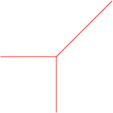
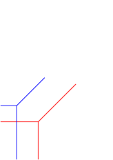
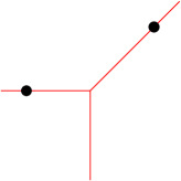
a)		b)		c)

Figure 1. The tropical line

What is even more important, although not at all visible from the picture, is that classical and tropical lines are both given by an equation of the form $ax+by+c=0$. In the realm of standard algebra, where addition is addition and multiplication is multiplication, we can determine without too much difficulty the classical line given by such an equation. In the tropical world, addition is replaced by the maximum and multiplication is replaced by addition. Just by doing this, all of our objects drastically change form! In fact, even “being equal to 0” takes on a very different meaning…

Classical and tropical geometries are developed following the same principles but from two different methods of calculation. They are simply the geometric faces of two different algebras.

Tropical geometry is not a game for bored mathematicians looking for something to do. In fact, the classical world can be degenerated to the tropical world in such a way so that the tropical objects conserve many properties of the original classical ones. Because of this, a tropical statement has a strong chance of having a similar classical analogue. The advantage is that tropical objects are piecewise linear and thus much simpler to study than their classical counterparts!

We could therefore summarise the approach of tropical geometry as follows:

Study simple objects to provide theorems concerning complicated objects.

The first part of this text focuses on tropical algebra, tropical curves and some of their properties. We then explain why classical and tropical geometries are related by showing how the classical world can be degenerated to the tropical one. We illustrate this principle by considering a method known as patchworking, which is used to construct real algebraic curves via objects called amoebas. Finally, in the last section we go beyond these topics to showcase some further developments in the field. These examples are a little more challenging than the rest of the text, as they illustrate more recent directions of research. We conclude by delivering some bibliographical references.

Before diving into the subject, we should explain the use of the word “tropical”. It is not due to the exotic forms of the objects under consideration, nor to the appearance of the previously mentioned “amoebas”. Before the term “tropical algebra”, the more cut-and-dry name of “max-plus algebra” was used. Then, in honour of the work of their Brazilian colleague, Imre Simon, the computer science researchers at the University of Paris 7 decided to trade the name of “max-plus” for “tropical”. Leaving the last word to Wikipedia, the origin of the word “tropical” simply reflects the French view on Brazil.

1. Tropical algebra

1.1. Tropical operations

Tropical algebra is the set of real numbers where addition is replaced by taking the maximum, and multiplication is replaced by the usual sum. In other words, we define two new operations on ${\mathbb{R}}$, called tropical addition and multiplication and denoted $``+"$ and $``\times"$ respectively, in the following way:

$$``x+y"=\max(x,y)\qquad``x\times y"=x+y$$

In this entire text, quotation marks will be placed around an expression to indicate that the operations should be regarded as tropical. Just as in classical algebra we often abbreviate $``x\times y"$ to $``xy"$. To familiarise ourselves with these two new strange operations, let’s do some simple calculations:

$${\text{``}}1+1{\text{''}}=1,\ \ {\text{``}}1+2{\text{''}}=2,\ \ {\text{``}}1+2+3{\text{''}}=3,\ \ {\text{``}}1\times 2{\text{''}}=3,\ \ {\text{``}}1\times(2+(-1)){\text{''}}=3,$$

$${\text{``}}1\times(-2){\text{''}}=-1,\ \ {\text{``}}(5+3)^{2}{\text{''}}=10.$$

These two tropical operations have many properties in common with the usual addition and multiplication. For example, they are both commutative and tropical multiplication $``\times"$ is distributive with respect to tropical addition $``+"$ (i.e. $``(x+y)z"=``xz+yz"$). There are however two major differences. First of all, tropical addition does not have an identity element in ${\mathbb{R}}$ (i.e. there is no element $x$ such that $\max\{y,x\}=y$ for all $y\in{\mathbb{R}}$). Nevertheless, we can naturally extend our two tropical operations to $-\infty$ by

$$\forall x\in{\mathbb{T}},\quad``x+(-\infty)"=\max(x,-\infty)=x\quad\text{and}\quad``x\times(-\infty)"=x+(-\infty)=-\infty,$$

where ${\mathbb{T}}={\mathbb{R}}\cup\{-\infty\}$ are the tropical numbers. Therefore, after adding $-\infty$ to ${\mathbb{R}}$, tropical addition now has an identity element. On the other hand, a major difference remains between tropical and classical addition: an element of ${\mathbb{R}}$ does not have an additive “inverse”. Said in another way, tropical subtraction does not exist. Neither can we solve this problem by adding more elements to ${\mathbb{T}}$ to try to cook up additive inverses. In fact, $``+"$ is said to be idempotent, meaning that $``x+x"=x$ for all $x$ in ${\mathbb{T}}$. Our only choice is to get used to the lack of tropical additive inverses!

Despite this last point, the tropical numbers ${\mathbb{T}}$ equipped with the operations $``+"$ and $``\times"$ satisfy all of the other properties of a field. For example, $0$ is the identity element for tropical multiplication, and every element $x$ of ${\mathbb{T}}$ different from $-\infty$ has a multiplicative inverse $``\frac{1}{x}"=-x$. Then ${\mathbb{T}}$ satisfies almost all of the axioms of a field, so by convention we say that it is a semi-field.

One must take care when writing tropical formulas! As, $``2x"\neq``x+x"$ but $``2x"=x+2$. Similarly, $``1x"\neq x$ but $``1x"=x+1$, and once again $``0x"=x$ and $``(-1)x"=x-1$.

1.2. Tropical polynomials

After having defined tropical addition and multiplication, we naturally come to consider functions of the form $P(x)=``\sum_{i=0}^{d}a_{i}x^{i}"$ with the $a_{i}$’s in ${\mathbb{T}}$, in other words, tropical polynomials. By rewriting $P(x)$ in classical notation, we obtain $P(x)=\max_{i=1}^{d}(a_{i}+ix)$. Let’s look at some examples of tropical polynomials:

$${\text{``}}x{\text{''}}=x,\ \ \ {\text{``}}1+x{\text{''}}=\max(1,x),\ \ \ {\text{``}}1+x+3x^{2}{\text{''}}=\max(1,x,2x+3),$$

$${\text{``}}1+x+3x^{2}+(-2)x^{3}{\text{''}}=\max(1,x,2x+3,3x-2).$$

Now let’s find the roots of a tropical polynomial. Of course, we must first ask, what is a tropical root? In doing this we encounter a recurring problem in tropical mathematics: a classical notion may have many equivalent definitions, yet when we pass to the tropical world these could turn out to be different, as we will see. Each equivalent definition of the same classical object potentially produces as many different tropical objects.

The most basic definition of classical roots of a polynomial $P(x)$ is an element $x_{0}$ such that $P(x_{0})=0$. If we attempt to replicate this definition in tropical algebra, we must look for elements $x_{0}$ in ${\mathbb{T}}$ such that $P(x_{0})=-\infty$. Yet, if $a_{0}$ is the constant term of the polynomial $P(x)$ then $P(x)\geq a_{0}$ for all $x$ in ${\mathbb{T}}$. Therefore, if $a_{0}\neq-\infty$, the polynomial $P(x)$ would not have any roots… This definition is surely not adequate.

We may take an alternative, yet equivalent, classical definition: an element, $x_{0}\in{\mathbb{T}}$ is a classical root of a polynomial $P(x)$ if there exists a polynomial $Q(x)$ such that $P(x)=(x-x_{0})Q(x)$. We will soon see that this definition is the correct one for tropical algebra. To understand it, let’s take a geometric point of view of the problem. A tropical polynomial is a piecewise linear function and each piece has an integer slope (see Figure 2). What is also apparent from the Figure 2 is that a tropical polynomial is convex, or “concave up”. This is because it is the maximum of a collection of linear functions.

We call tropical roots of the polynomial $P(x)$ all points $x_{0}$ of ${\mathbb{T}}$ for which the graph of $P(x)$ has a corner at $x_{0}$. Moreover, the difference in the slopes of the two pieces adjacent to a corner gives the order of the corresponding root. Thus, the polynomial $``0+x"$ has a simple root at $x_{0}=0$, the polynomial $``0+x+(-1)x^{2}{\text{''}}$ has simple roots $0$ and $1$ and the polynomial $``0+x^{2}{\text{''}}$ has a double root at $0$.

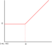
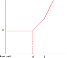
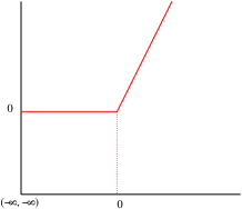
a) $P(x)={\text{``}}0+x{\text{''}}$		b) $P(x)={\text{``}}0+x+(-1)x^{2}{\text{''}}$		b) $P(x)={\text{``}}0+x^{2}{\text{''}}$

Figure 2. The graphs of some tropical polynomials

The roots of a tropical polynomial $P(x)={\text{``}}\sum_{i=0}^{d}a_{i}x^{i}{\text{''}}=\max_{i=1}^{d}(a_{i}+ix)$ are therefore exactly the tropical numbers $x_{0}$ for which there exists a pair $i\neq j$ such that $P(x_{0})=a_{i}+ix_{0}=a_{j}+jx_{0}$. We say that the maximum of $P(x)$ is obtained (at least) twice at $x_{0}$. In this case, the order of the root at $x_{0}$ is the maximum of $|i-j|$ for all possible pairs $i$, $j$ which realise this maximum at $x_{0}$. For example, the maximum of $P(x)={\text{``}}0+x+x^{2}{\text{''}}$ is obtained 3 times at $x_{0}=0$ and the order of this root is 2. Equivalently, $x_{0}$ is a tropical root of order at least $k$ of $P(x)$ if there exists a tropical polynomial $Q(x)$ such that $P(x)={\text{``}}(x+x_{0})^{k}Q(x){\text{''}}$. Note that the factor $x-x_{0}$ in classical algebra gets transformed to the factor ${\text{``}}x+x_{0}{\text{''}}$, since the root of the polynomial ${\text{``}}x+x_{0}{\text{''}}$ is $x_{0}$ and not $-x_{0}$.

This definition of a tropical root seems to be much more satisfactory than the first one. In fact, using this definition we have the following proposition.

Proposition 1.1.

The tropical semi-field is algebraically closed. In other words, every tropical polynomial of degree $d$ has exactly $d$ roots when counted with multiplicities.

For example, one may check that we have the following factorisations:

$${\text{``}}0+x+(-1)x^{2}{\text{''}}={\text{``}}(-1)(x+0)(x+1){\text{''}}\ \ \ and\ \ \ {\text{``}}0+x^{2}{\text{''}}={\text{``}}(x+0)^{2}{\text{''}}$$

1.3. Exercises

1. Why does the idempotent property of tropical addition prevent the existence of inverses for this operation?

2. Draw the graphs of the tropical polynomials $P(x)={\text{``}}x^{3}+2x^{2}+3x+(-1){\text{''}}$ and $Q(x)={\text{``}}x^{3}+(-2)x^{2}+2x+(-1){\text{''}}$, and determine their tropical roots.

3. Let $a\in{\mathbb{R}}$ and $b,c\in{\mathbb{T}}$. Determine the roots of the polynomials ${\text{``}}ax+b{\text{''}}$ and ${\text{``}}ax^{2}+bx+c{\text{''}}$.

4. Prove that $x_{0}$ is a tropical root of order at least $k$ of $P(x)$ if and only if there exists a tropical polynomial $Q(x)$ such that $P(x)={\text{``}}(x+x_{0})^{k}Q(x){\text{''}}$.

5. Prove Proposition 1.1.

2. Tropical curves

2.1. Definition

Carrying on boldly, we can increase the number of variables in our polynomials. A tropical polynomial in two variables is written $P(x,y)={\text{``}}\sum_{i,j}a_{i,j}x^{i}y^{j}{\text{''}}$, or better yet $P(x,y)=\max_{i,j}(a_{i,j}+ix+jy)$ in classical notation. In this way our tropical polynomial is again a convex piecewise linear function, and the tropical curve $C$ defined by $P(x,y)$ is the corner locus of this function. Said in another way, a tropical curve $C$ consists of all points $(x_{0},y_{0})$ in ${\mathbb{T}}^{2}$ for which the maximum of $P(x,y)$ is obtained at least twice at $(x_{0},y_{0})$.

We should point out that up until Section 6 we will focus on tropical curves contained in ${\mathbb{R}}^{2}$ and not in ${\mathbb{T}}^{2}$. This does not affect at all the generality of what will be discussed here, however it renders the definitions, the statements, and our drawings simpler and easier to understand.

Let us look at the tropical line defined by the polynomial $P(x,y)={\text{``}}\frac{1}{2}+2x+(-5)y{\text{''}}$. We must find the points $(x_{0},y_{0})$ in ${\mathbb{R}}^{2}$ that satisfy one of the following three systems of equations:

$$2+x_{0}=\frac{1}{2}\geq-5+y_{0},\ \ \ \ \ \ \ \ \ -5+y_{0}=\frac{1}{2}\geq 2+x_{0},\ \ \ \ \ \ \ \ \ 2+x_{0}=-5+y_{0}\geq\frac{1}{2}.$$

We see that our tropical line is made up of three standard half-lines

$$\{(-\frac{3}{2},y)\ |\ y\leq\frac{11}{2}\},\ \{(x,\frac{11}{2})\ |\ x\leq-\frac{3}{2}\},\text{ and }\{(x,x+7)\ |\ x\geq-\frac{3}{2}\}$$

(see Figure 3a).

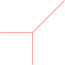
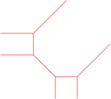
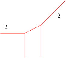
a) ${\text{``}}\frac{1}{2}+2x+(-5)y{\text{''}}$	b) ${\text{``}}3+2x+2y+3xy+y^{2}+x^{2}{\text{''}}$	c) ${\text{``}}0+x+y+y^{2}+(-1)x^{2}{\text{''}}$

Figure 3. Some tropical curves

We are still missing one bit of information to properly define a tropical curve. The corner locus of a tropical polynomial in two variables consists of line segments and half-lines, which we call edges. These intersect at points which we will call vertices. Just as in the case of polynomials in one variable, for each edge of a tropical curve, we must take into account the difference in the slope of $P(x,y)$ on the two sides of the edge. Doing this, we arrive at the following formal definition of a tropical curve.

Definition 2.1.

Let $P(x,y)={\text{``}}\sum_{i,j}a_{i,j}x^{i}y^{j}{\text{''}}$ be a tropical polynomial. The tropical curve $C$ defined by $P(x,y)$ is the set of points $(x_{0},y_{0})$ of ${\mathbb{R}}^{2}$ such that there exists pairs $(i,j)\neq(k,l)$ satisfying $P(x_{0},y_{0})=a_{i,j}+ix_{0}+jy_{0}=a_{k,l}+kx_{0}+ly_{0}$.

We define the weight $w_{e}$ of an edge $e$ of $C$ to be the maximum of the greatest common divisor (gcd) of the numbers $|i-k|$ and $|j-l|$ for all pairs $(i,j)$ and $(k,l)$ which correspond to this edge. That is to say,

$$w_{e}=\max_{M_{e}}\left(\gcd(|i-k|,|j-l|)\right),$$

where

$$M_{e}=\{(i,j),(k,l)\ |\ \forall x_{0}\in e,P(x_{0},y_{0})=a_{i,j}+ix_{0}+jy_{0}=a_{k,l}+kx_{0}+ly_{0}\}.$$

In Figure 3, the weight of an edge is only indicated if the weight is at least two. For example, in the case of the tropical line, all edges are of weight 1. Thus, Figure 3a represents fully the tropical line. Two examples of tropical curves of degree 2 are shown in Figure 3b and c. The tropical conic in Figure 3c has two edges of weight 2. Note that given an edge $e$ of a tropical curve defined by $P(x,y)$, the set $M_{e}$ can have any cardinality between $2$ and $w_{e}+1$: in the example of Figure 3c, we have $M_{e}=\{(0,0),(0,1),(0,2)\}$ if $e$ is the horizontal edge, and $M_{e}=\{(2,0),(0,2)\}$ if $e$ is the other edge of weight $2$.

2.2. Dual subdivisions

To recap, a tropical polynomial is given by the maximum of a finite number of linear functions corresponding to monomials of $P(x,y)$. Moreover, the points of the plane ${\mathbb{R}}^{2}$ for which at least two of these monomials realise the maximum are exactly the points of the tropical curve $C$ defined by $P(x,y)$. Let us refine this a bit and consider at each point $(x_{0},y_{0})$ of $C$, all of the monomials of $P(x,y)$ that realise the maximum at $(x_{0},y_{0})$.

Let us first go back to the tropical line $C$ defined by the equation $P(x,y)={\text{``}}\frac{1}{2}+2x+(-5)y{\text{''}}$ (see Figure 3a). The point $(-\frac{3}{2},\frac{11}{2})$ is the vertex of the line $C$. This is where the three monomials $\frac{1}{2}=\frac{1}{2}x^{0}y^{0}$, $2x=2x^{1}y^{0}$ and $(-5)y=(-5)x^{0}y^{1}$ take the same value. The exponents of those monomials, that it to say the points $(0,0)$, $(1,0)$ and $(0,1)$, define a triangle $\Delta_{1}$ (see Figure 4a). Along the horizontal edge of $C$ the value of the polynomial $P(x,y)$ is given by the monomials $0$ and $y$, in other words, the monomials with exponents $(0,0)$ and $(0,1)$. Therefore, these two exponents define the vertical edge of the triangle $\Delta_{1}$. In the same way, the monomials giving the value of $P(x,y)$ along the vertical edge of $C$ have exponents $(0,0)$ and $(1,0)$, which define the horizontal edge of $\Delta_{1}$. Finally, along the edge of $C$ that has slope 1, $P(x,y)$ is given by the monomials with exponents $(1,0)$ and $(0,1)$, which define the edge of $\Delta_{1}$ that has slope $-1$.

What can we learn from this digression? In looking at the monomials which give the value of the tropical polynomial $P(x,y)$ at a point of the tropical line $C$, we notice that the vertex of $C$ corresponds to the triangle $\Delta_{1}$ and that each edge $e$ of $C$ corresponds to an edge $\delta_{e}$ of $\Delta_{1}$, whose direction is perpendicular to that of $e$.

Let us illustrate this with the tropical conic defined by the polynomial $P(x,y)={\text{``}}3+2x+2y+3xy+x^{2}+y^{2}{\text{''}}$, and drawn in Figure 3b. This curve has as its vertices four points $(-1,1)$, $(-1,2)$, $(1,-1)$ and $(2,-1)$. At each of these vertices $(x_{0},y_{0})$, the value of the polynomial $P(x,y)$ is given by three monomials:

$$P(-1,1)=3=y_{0}+2=x_{0}+y_{0}+3\ \ \ \ \ \ \ \ \ \ \ \ \ \ \ \ P(-1,2)=y_{0}+2=x_{0}+y_{0}+3=2y_{0}\ \$$

$$P(1,-1)=3=x_{0}+2=x_{0}+y_{0}+3\ \ \ \ \ \ \ \ \ \ \ \ \ \ \ \ P(2,-1)=x_{0}+2=x_{0}+y_{0}+3=2x_{0}.\ \$$

Thus for each vertex of $C$, the exponents of the three corresponding monomials define a triangle, and these four triangles are arranged as shown in Figure 4b. Moreover, just as in the case of the line, for each edge $e$ of $C$, the exponents of the monomials giving the value of $P(x,y)$ along the edge $e$ define an edge of one (or two) of these triangles. Once again the direction of the edge $e$ is perpendicular to the corresponding edge of the triangle.

To explain this phenomenon in full generality, let $P(x,y)={\text{``}}\sum_{i,j}a_{i,j}x^{i}y^{j}{\text{''}}$ be any tropical polynomial. The degree of $P(x,y)$ is the maximum of the sums $i+j$ for all coefficients $a_{i,j}$ different from $-\infty$. For simplicity, we will assume in this text that all polynomials of degree $d$ satisfy $a_{0,0}\neq-\infty$, $a_{d,0}\neq-\infty$ and $a_{0,d}\neq-\infty$. Thus, all the points $(i,j)$ such that $a_{i,j}\neq-\infty$ are contained in the triangle with vertices $(0,0)$, $(0,d)$ and $(d,0)$, which we call $\Delta_{d}$. Given a finite set of points $A$ in ${\mathbb{R}}^{2}$, the convex hull of $A$ is the unique convex polygon with vertices in $A$ and containing $A$. From what we just said, the triangle $\Delta_{d}$ is precisely the convex hull of the points $(i,j)$ such that $a_{i,j}\neq-\infty$.

If $v=(x_{0},y_{0})$ is a vertex of the curve $C$ defined by $P(x,y)$, then the convex hull of the points $(i,j)$ in $\Delta_{d}\cap{\mathbb{Z}}^{2}$ such that $P(x_{0},y_{0})=a_{i,j}+ix_{0}+jy_{0}$ is another polygon $\Delta_{v}$ which is contained in $\Delta_{d}$. Similarly, if $(x_{0},y_{0})$ is a point in the interior of an edge $e$ of $C$, then the convex hull of the points $(i,j)$ in $\Delta_{d}\cap{\mathbb{Z}}^{2}$ such that $P(x_{0},y_{0})=a_{i,j}+ix_{0}+jy_{0}$ is a segment $\delta_{e}$ contained in $\Delta_{d}$. The fact that the tropical polynomial $P(x,y)$ is a convex piecewise linear function implies that the collection of all $\Delta_{v}$ form a subdivision of $\Delta_{d}$. In other words, the union of all of the polygons $\Delta_{v}$ is equal to the triangle $\Delta_{d}$, and two polygons $\Delta_{v}$ and $\Delta_{v^{\prime}}$ have either an edge in common, a vertex in common, or do not intersect at all. Moreover, if $e$ is an edge of $C$ adjacent to the vertex $v$, then $\delta_{e}$ is an edge of the polygon $\Delta_{v}$, and $\delta_{e}$ is perpendicular to $e$. In particular, an edge $e$ of $C$ is infinite, i.e. is adjacent to only one vertex of $C$, if and only if $\Delta_{e}$ is contained in an edge of $\Delta_{d}$. This subdivision of $\Delta_{d}$ is called the dual subdivision of $C$.

For example, the dual subdivisions of the tropical curves in Figure 3 are drawn in Figure 4 (the black points represent the points of ${\mathbb{R}}^{2}$ with integer coordinates; notice they are not necessarily the vertices of the dual subdivision).

The weight of an edge may be read off directly from the dual subdivision.

Proposition 2.2.

An edge $e$ of a tropical curve has weight $w$ if and only if $Card(\Delta_{e}\cap{\mathbb{Z}}^{2})=w+1$.

It follows from Proposition 2.2 that the degree of a tropical curve may be determined easily only from the curve itself: it is the sum of weights of all infinite the edges in the direction $(-1,0)$ (we could equally consider the directions $(0,-1)$ or $(1,1)$). Moreover, up to a translation and choice of lengths of its edges, a tropical curve is determined by its dual subdivision.

a)		b)		c)

Figure 4. Some dual subdivisions

2.3. Balanced graphs and tropical curves.

The first consequence of the duality from the last section is that a certain relation, known as the balancing condition, is satisfied at each vertex of a tropical curve. Suppose $v$ is a vertex of $C$ adjacent to the edges $e_{1},\dots,e_{k}$ with respective weights $w_{1},\dots,w_{k}$. Recall that every edge $e_{i}$ is contained in a line (in the usual sense) defined by an equation with integer coefficients. Because of this there exists a unique integer vector $\vec{v}_{i}=(\alpha,\beta)$ in the direction of $e_{i}$ such that $\text{gcd}(\alpha,\beta)=1$ (see Figure 5a). We orient the boundary of $\Delta_{v}$ in the counter-clockwise direction, so that each edge $\delta_{e_{i}}$ of $\Delta_{v}$ dual to $e_{i}$ is obtained from a vector $w_{i}\vec{v}_{i}$ by rotating by an angle of exactly $\pi/2$ (see Figure 5b). Then, following the previous section, the polygon $\Delta_{v}$ dual to $v$ yields immediately the vectors $w_{1}\vec{v}_{1},\dots,w_{k}\vec{v}_{k}$.

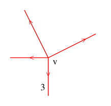
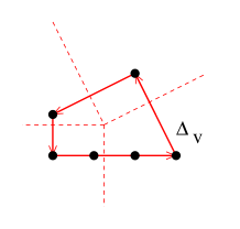
a)		b)

Figure 5. Balancing condition

The fact that the polygon $\Delta_{v}$ is closed immediately implies the following balancing condition:

$$\sum_{i=1}^{k}w_{i}\vec{v}_{i}=0.$$

A graph in ${\mathbb{R}}^{2}$ whose edges have rational slopes and are equipped with positive integer weights is a balanced graph if it satisfies the balancing condition at each one of its vertices. We have just seen that every tropical curve is a balanced graph. In fact, the converse is also true.

Theorem 2.3 (G. Mikhalkin).

Tropical curves in ${\mathbb{R}}^{2}$ are exactly the balanced graphs.

Thus, this theorem affirms that there exist tropical polynomials of degree 3 whose tropical curves are the weighted graphs in Figure 6. We have also drawn for each curve, the associated dual subdivision of $\Delta_{3}$.

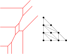
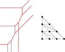
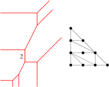
a)		b)		c)

Figure 6.

2.4. Exercises

1. Draw the tropical curves defined by the tropical polynomials $P(x,y)={\text{``}}5+5x+5y+4xy+1y^{2}+x^{2}{\text{''}}$ and $Q(x,y)={\text{``}}7+4x+y+4xy+3y^{2}+(-3)x^{2}{\text{''}}$, as well as their dual subdivisions.

2. A tropical triangle is a domain of ${\mathbb{R}}^{2}$ bounded by three tropical lines. What are the possible forms of a tropical triangle?

3. Prove Proposition 2.2.

4. Show that a tropical curve of degree $d$ has at most $d^{2}$ vertices.

5. Find an equation for each of the tropical curves in Figure 6. The following reminder might be helpful: if $v$ is a vertex of a tropical curve defined by a tropical polynomial $P(x,y)$, then the value of $P(x,y)$ in a neighbourhood of $v$ is given uniquely by the monomials corresponding to the polygon dual to $v$.

3. Tropical intersection theory

3.1. Bézout’s theorem.

One of the main interests of tropical geometry is to provide a simple model of algebraic geometry. For example, the basic theorems from intersection theory of tropical curves require much less mathematical background than their classical counterparts. The theorem which we have in mind is Bézout’s theorem, which states that two algebraic curves in the plane of degrees $d_{1}$ and $d_{2}$ respectively, intersect in $d_{1}d_{2}$ points. Before we tackle the general case, let us first consider tropical lines and conics.

As mentioned in the introduction, most of the time two tropical lines intersect in exactly one point (see Figure 7a), just as in classical geometry. Now, do a tropical line and a tropical conic intersect each other in two points? If we naively count the number of intersection points, the answer is sometimes yes (Figure 7b) and sometimes no (Figure 7c)…

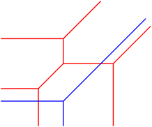
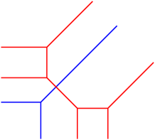
a)		b)		c)

Figure 7. Intersections of tropical lines and conics

In fact, the unique intersection point of the conic and the tropical line in Figure 7c should be counted twice. But why twice in this case and not in the previous case? To find the answer we look to the dual subdivisions.

We start by restricting to the case when the curves $C_{1},C_{2}$ intersect in a finite collection of points away from the vertices of both curves. Remark that the union of the two tropical curves $C_{1}$ and $C_{2}$ is again a tropical curve. In fact, we can easily verify that the union of two balanced graphs is again a balanced graph. Or, we could also easily check that if $C_{1}$ and $C_{2}$ are defined by tropical polynomials $P_{1}(x,y)$, $P_{2}(x,y)$ respectively, then $Q(x,y)=``P_{1}(x,y)P_{2}(x,y)"$ defines precisely the curve $C_{1}\cup C_{2}$. Moreover, the degree of $C_{1}\cup C_{2}$ is the sum of the degrees of $C_{1}$ and $C_{2}$.

The dual subdivisions of the unions of the two curves $C_{1}$ and $C_{2}$ in the three cases of Figure 7 are represented in Figure 8. In every case, the set of vertices of $C_{1}\cup C_{2}$ is the union of the vertices of $C_{1}$, the vertices of $C_{2}$, and of the intersection points of $C_{1}$ and $C_{2}$. Moreover, since each point of intersection of $C_{1}$ and $C_{2}$ is contained in an edge of both $C_{1}$ and $C_{2}$, the polygon dual to such a vertex of $C_{1}\cup C_{2}$ is a parallelogram. To make Figure 8 more transparent, we have drawn each edge of the dual subdivision in the same colour as its corresponding dual edge. We can conclude that in Figures 8a and b, the corresponding parallelograms are of area one, whereas the corresponding parallelogram of the dual subdivision in Figure 8c has area two! Hence, it seems that we are counting each intersection point with the multiplicity we will describe below.

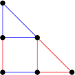
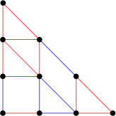
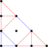
a)		b)		c)

Figure 8. The subdivisions dual to the union of the curves in Figure 7

Definition 3.1.

Let $C_{1}$ and $C_{2}$ be two tropical curves which intersect in a finite number of points and away from the vertices of the two curves. If $p$ is a point of intersection of $C_{1}$ and $C_{2}$, the tropical multiplicity of $p$ as an intersection point of $C_{1}$ and $C_{2}$ is the area of the parallelogram dual to $p$ in the dual subdivision of $C_{1}\cup C_{2}$.

With this definition, proving the tropical Bézout’s theorem is a walk in the park!

Theorem 3.2 (B. Sturmfels).

Let $C_{1}$ and $C_{2}$ be two tropical curves of degrees $d_{1}$ and $d_{2}$ respectively, intersecting in a finite number of points away from the vertices of the two curves. Then the sum of the tropical multiplicities of all points in the intersection of $C_{1}$ and $C_{2}$ is equal to $d_{1}d_{2}$.

Proof.

Let us call this sum of multiplicities $s$. Notice that there are three types of polygons in the subdivision dual to the tropical curve $C_{1}\cup C_{2}$:

• those which are dual to a vertex of $C_{1}$. The sum of their areas is equal to the area of $\Delta_{d_{1}}$, in other words $\frac{d_{1}^{2}}{2}$,

• those which are dual to a vertex of $C_{2}$. The sum of their areas is equal to $\frac{d_{2}^{2}}{2}$,

• those dual to a intersection point of $C_{1}$ and $C_{2}$. The sum of their areas we have called $s$.

Since the curve $C_{1}\cup C_{2}$ is of degree $d_{1}+d_{2}$, the sum of the area of all of these polygons is equal to the area of $\Delta_{d_{1}+d_{2}}$, which is $\frac{(d_{1}+d_{2})^{2}}{2}$. Therefore, we obtain

$$s=\frac{(d_{1}+d_{2})^{2}-d_{1}^{2}-d_{2}^{2}}{2}=d_{1}d_{2},$$

which completes the proof. ∎

3.2. Stable intersection

In the last section we considered only tropical curves which intersect “nicely”, meaning they intersect only in a finite number of points and away from the vertices of the two curves. But what can we say in the two cases shown in the Figures 9a (two tropical lines that intersect in an edge) and 9b (a tropical line passing through a vertex of a conic)? Thankfully, we have more than one tropical trick up our sleeve.

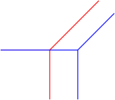
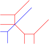
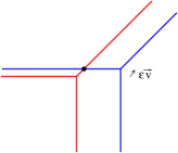
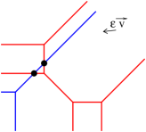
a)		b)		c)		d)

Figure 9. Non-transverse intersection and a translation

Let $\varepsilon$ be a very small positive real number and $\vec{v}$ a vector such that the quotient of its two coordinates is an irrational number. If we translate in each of the two cases one of the two curves in Figure 9a and b by the vector $\varepsilon\vec{v}$, we find ourselves back in the case of “nice” intersection (see Figures 9c and d). Of course, the resulting intersection depends on the vector $\varepsilon\vec{v}$. But on the other hand, the limit of these points, if we let $\varepsilon$ shrink to 0, does not depend on $\vec{v}$. The points in the limit are called the stable intersection points of two curves. The multiplicity of a point $p$ in the stable intersection is equal to the sum of the intersection multiplicities of all points which converge to $p$ when $\varepsilon$ tends to zero.

For example, there is only one stable intersection point of the two lines in Figure 9a. The point is the vertex of the line on the left. Moreover, this point has multiplicity 1, so again, our two tropical lines intersect in a single point. The point of stable intersection of the two curves in Figure 9b is the vertex of the conic, and it has multiplicity 2.

Notice that if a point is in the stable intersection of two tropical curves it is either an isolated intersection point, or a vertex of one of the two curves. Thanks to stable intersection, we can remove from our previous statement of the tropical Bézout theorem the hypothesis that the curves must intersect “nicely”.

Theorem 3.3 (B. Sturmfels).

Let $C_{1}$ and $C_{2}$ be two tropical curves of degree $d_{1}$ and $d_{2}$. Then the sum of the multiplicities of the stable intersection points of $C_{1}$ and $C_{2}$ is equal to $d_{1}d_{2}$.

In passing, we may notice a surprising tropical phenomenon: a tropical curve has a well defined self-intersection! Indeed, all we have to do is to consider the stable intersection of a tropical curve with itself. Following the discussion above, the self-intersection points of a curve are the vertices of the curve. (see Figure 10).

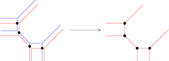
Figure 10. The 4 points in the self-intersection of a conic

3.3. Exercises

1. Determine the stable intersection points of the two tropical curves in Exercise 1 of Section 2, as well as their multiplicity.

2. A double point of a tropical curve is a point where two edges intersect (i.e. the dual polygon to the vertex of the curve is a parallelogram). Show that a tropical conic with a double point is the union of two tropical lines. Hint: consider a line passing through the double point of the conic and any other vertex of the conic.

3. Show that a tropical curve of degree 3 with two double points is the union of a line and a tropical conic. Show that a tropical curve of degree 3 with 3 double points is the union of 3 tropical lines.

4. A few explanations

Let us pause for a while with our introduction of tropical geometry to explain briefly some connections between classical and tropical geometry. In particular, our goal is to illustrate the fact that tropical geometry is a limit of classical geometry. If we were to summarise roughly the content of this section in one sentence it would be: tropical geometry is the image of classical geometry under the logarithm with base $+\infty$.

4.1. Maslov dequantisation.

First of all let us explain how the tropical semi-field arises naturally as the limit of some classical semi-fields. This procedure, studied by Victor Maslov and his collaborators beginning in the 90’s, is known as dequantisation of the real numbers.

A well-known semi-field is the set of positive or zero real numbers together with the usual addition and multiplication, denoted $({\mathbb{R}}_{+},+,\times)$. If $t$ is a strictly positive real number, then the logarithm of base $t$ provides a bijection between the sets ${\mathbb{R}}$ and ${\mathbb{T}}$. This bijection induces a semi-field structure on ${\mathbb{T}}$ with the operations denoted by ${\text{``}}+_{t}{\text{''}}$ and ${\text{``}}\times_{t}{\text{''}}$, and given by:

$${\text{``}}x+_{t}y{\text{''}}=\log_{t}(t^{x}+t^{y})\ \ \ \text{ and }\ \ \ {\text{``}}x\times_{t}y{\text{''}}=\log_{t}(t^{x}t^{y})=x+y.$$

The equation on the right-hand side already shows classical addition appearing as an exotic kind of multiplication on ${\mathbb{T}}$. Notice that by construction, all of the semi-fields $({\mathbb{T}},{\text{``}}+_{t}{\text{''}},{\text{``}}\times_{t}{\text{''}})$ are isomorphic to $({\mathbb{R}}_{+},+,\times)$. The trivial inequality $\max(x,y)\leq x+y\leq 2\max(x,y)$ on ${\mathbb{R}}_{+}$ together with the fact that the logarithm is an increasing function gives us the following bounds for ${\text{``}}+_{t}{\text{''}}$:

$$\forall t>1,\ \ \max(x,y)\leq{\text{``}}x+_{t}y{\text{''}}\leq\max(x,y)+\log_{t}2.$$

If we let $t$ tend to infinity, then $\log_{t}2$ tends to $0$, and the operation ${\text{``}}+_{t}{\text{''}}$ therefore tends to the tropical addition ${\text{``}}+{\text{''}}$! Hence the tropical semi-field comes naturally from degenerating the classical semi-field $({\mathbb{R}}_{+},+,\times)$. From an alternative perspective, we can view the classical semi-field $({\mathbb{R}}_{+},+,\times)$ as a deformation of the tropical semi-field. This explains the use of the term “dequantisation”, coming from physics and referring to the procedure of passing from quantum to classical mechanics.

4.2. Dequantisation of a line in the plane.

Now we will apply a similar reasoning to the line in the plane ${\mathbb{R}}^{2}$ defined by the equation $x-y+1$ (see Figure 11a). To apply the logarithm map to the coordinates of ${\mathbb{R}}^{2}$, we must first take their absolute values. Doing this results in folding the 4 quadrants of ${\mathbb{R}}^{2}$ onto the positive quadrant (see Figure 11b). The image of the folded up line under the coordinate-wise logarithm with base $t$ applied to $({\mathbb{R}}_{+}^{*})^{2}$ is drawn in Figure 11c. By definition, taking the logarithm with base $t$ is the same thing as taking the natural logarithm and then rescaling the result by a factor of $\frac{1}{\ln t}$. Thus, as $t$ increases, the image under the logarithm with base $t$ of the absolute value of our line becomes concentrated around a neighbourhood of the origin and three asymptotic directions, as shown in Figures 11c, d and e. If we allow $t$ go all the way to infinity, then we see the appearance in Figure 11f of… a tropical line!

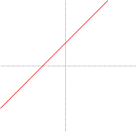
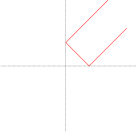
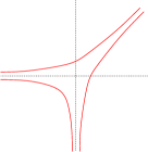
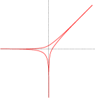
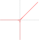
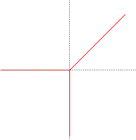
a)	b)	c)	d)	e)	f)

Figure 11. Dequantisation of a line

5. Patchworking

In reading Figure 11 from left to right, we see how starting from a classical line in the plane we can arrive at a tropical line. Reading this figure from right to left is in fact much more interesting! Indeed, we see as well how to construct a classical line given a tropical one. The technique known as patchworking is a generalisation of this observation. In particular, it provides a purely combinatorial procedure to construct real algebraic curves from a tropical curve. In order to explain this procedure in more detail, we first go a bit back in time.

5.1. Hilbert’s 16th problem.

A planar real algebraic curve is a curve in the plane ${\mathbb{R}}^{2}$ defined by an equation of the form $P(x,y)=0$, where $P(x,y)$ is a polynomial whose coefficients are real numbers. The real algebraic curves of degree 1 and 2 are simple and well-known; they are lines and conics respectively. When the degree of $P(x,y)$ increases, the form of the real algebraic curve can become more and more complicated. If you are not convinced, take a look at figure 12 which shows some of the possible drawings realised by real algebraic curves of degree 4.

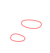
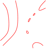
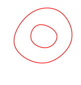
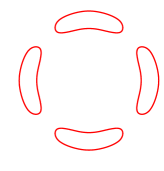
a)		b)		c)		d)

Figure 12. Some real algebraic curves of degree 4

A theorem due to Axel Harnack at the end of the XIXth century states that a planar real algebraic curve of degree $d$ has a maximum of $\frac{d(d-1)+2}{2}$ connected components. But how can these components be arranged with respect to each other? We call the relative position of the connected components of a planar real algebraic curve in the plane its arrangement. In other words, we are not interested in the exact position of the curve in the plane, but simply in the configuration that it realises. For example, if one curve has two bounded connected components, we are only interested in whether one of these components is contained in the other (Figure 12c) or not (Figure 12a). At the second International Congress in Mathematics in Paris in 1900, David Hilbert announced his famous list of 23 problems for the XXth century. The first part of his 16th problem can be very widely understood as the following:

Given a positive integer $d$, establish a list of possible arrangements of real algebraic curves of degree $d$.

At Hilbert’s time, the answer was known for curves of degree at most 4. There have been spectacular advances in this problem in the XXth century due mostly in part to mathematicians from the Russian school. Despite this, there remain numerous open questions…

5.2. Real and tropical curves

In general, it is a difficult problem to construct a real algebraic curve of a fixed degree and realising a given arrangement. For a century, mathematicians have proposed many ingenious methods for doing this. The patchworking method invented by Oleg Viro in the 70’s is actually one of the most powerful. At this time, tropical geometry was not yet in existence, and Viro announced his theorem in a language different from what we use here. However, he realised by the end of the 90’s that his patchworking could be interpreted as a quantisation of tropical curves. Patchworking is in fact the process of reading Figure 11 from right to left instead of left to right. Thanks to the interpretation of patchworking in terms of tropical curves, shortly afterwards, Grigory Mikhalkin generalised Viro’s original method. Here we will present a simplified version of patchworking. The interested reader may find a more complete version in the references indicated at the end of the text in Section 7.

In what follows, for $a$, $b$ two integer numbers, we denote by $s_{a,b}:{\mathbb{R}}^{2}\to{\mathbb{R}}^{2}$ the composition of $a$ reflections in the $x$-axis with $b$ reflections in the $y$-axis. Therefore, the map $s_{a,b}$ depends only on the parity of $a$ and $b$. To be precise, $s_{0,0}$ is the identity, $s_{1,0}$ is the reflection in the $x$-axis, $s_{0,1}$ reflection in the $y$-axis, and $s_{1,1}$ is reflection in the origin (equivalently, rotation by 180 degrees).

We will now explain in detail the procedure of patchworking. We start with a tropical curve $C$ of degree $d$ which has only edges of odd weight, and such that the polygons dual to all vertices are triangles. For example, take the tropical line from Figure 13a. For each edge $e$ of $C$, choose a vector $\vec{v}_{e}=(\alpha_{e},\beta_{e})$ in the direction of $e$ such that $\alpha_{e}$ and $\beta_{e}$ are relatively prime integers (note that we may choose either $\vec{v}_{e}$ or $-\vec{v}_{e}$, but this does not matter in what follows). For the tropical line, we may take the vectors $(1,0)$, $(0,1)$ and $(1,1)$. Now let us think of the plane ${\mathbb{R}}^{2}$ where our tropical curve sits as being the positive quadrant $({\mathbb{R}}^{*}_{+})^{2}$ of ${\mathbb{R}}^{2}$, and take the union of the curve with its 3 symmetric copies obtained by reflections in the axes. For the tropical line, we obtain Figure 13b. For each edge $e$ of our curve, we will erase two out of the four symmetric copies of $e$, denoted $e^{\prime}$ and $e^{\prime\prime}$. Our choice must satisfy the following rules:

• $e^{\prime}=s_{\alpha_{e},\beta_{e}}(e^{\prime\prime})$,

• for each vertex $v$ of $C$ adjacent to the edges $e_{1}$, $e_{2}$ and $e_{3}$ and for each pair $(\varepsilon_{1},\varepsilon_{2})$ in $\{0,1\}^{2}$, exactly one or three of the copies of $s_{\varepsilon_{1},\varepsilon_{2}}(e_{1})$, $s_{\varepsilon_{1},\varepsilon_{2}}(e_{2})$, and $s_{\varepsilon_{1},\varepsilon_{2}}(e_{3})$ are erased.

We call the result after erasing the edges a real tropical curve. For example, if $C$ is a tropical line, using the rules above, it is possible to erase 6 of the edges from the symmetric copies of $C$ to obtain the real tropical line represented in Figure 13c. It is true that this real tropical curve is not a regular line in ${\mathbb{R}}^{2}$, but they are arranged in the plane in same way (see Figure 13d)!

This is not just a coincidence, it is in fact a theorem.

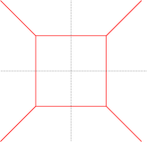
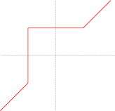
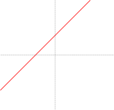
a)		b)		c)		d)

Figure 13. Patchworking of a line

Theorem 5.1 (O. Viro).

Given any real tropical curve of degree $d$, there exists a real algebraic curve of degree $d$ with the same arrangement.

We should take a second to realise the depth and elegance of the above statement. A real tropical curve is constructed by following the rules of a purely combinatorial game. It seems like magic to assert that there is a relationship between these combinatorial objects and actual real algebraic curves! We will not get into details here, but Viro’s method even allows us to determine the equation of a real algebraic curve with the same arrangement than a given real tropical curve.

Of course, much skill and intuition are still required to construct real algebraic curves with complicated arrangements and both of these are acquired with practice. Therefore, we invite the reader to try the exercises at the end of this section. Nevertheless, patchworking provides a much more flexible technique to construct arrangements than dealing directly with polynomials, in particular it requires a priori no knowledge in algebraic geometry. To illustrate the use of Viro’s patchworking, let us now construct the arrangements of two real algebraic curves, one of degree 3 and the other of degree 6.

First of all, consider the tropical curve of degree 3 shown in Figure 14a. For suitable choices of edges to erase, the Figures 14b and c represent the two stages of the patchworking procedure. With this we have proved the existence of a real algebraic curve of degree 3 resembling the configuration of Figure 14d.

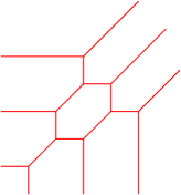
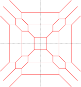
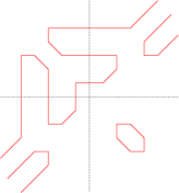
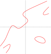
a)		b)		c)		d)

Figure 14. Patchworking of a cubic

To finish, consider the tropical curve of degree 6 drawn in Figure 15a. Once again, for a suitable choice of edges to erase, the patchworking procedure gives the curve in Figure 15c. A real algebraic curve of degree 6 which realises the same arrangement as the real tropical curve was first constructed using much more complicated techniques in the 60’s by Gudkov. An interesting piece of trivia: Hilbert announced in 1900 that such a curve could not exist!

5.3. Amoebas

Even though dequantisation of a line is the main idea underlying patchworking in its full generality, the proof of Viro’s theorem is quite a bit more technical to explain rigorously. Here we will give a sketch of what is involved in the proof.

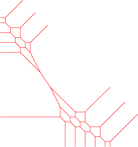
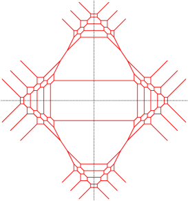
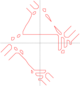
a)	b)	c)

Figure 15. Gudkov’s curve

First of all, since the field ${\mathbb{R}}$ is not algebraically closed, we will not work with real algebraic curves but rather complex algebraic curves. In other words, subsets of the space $({\mathbb{C}}^{*})^{2}$ defined by equations of the form $P(x,y)=0$, where ${\mathbb{C}}^{*}={\mathbb{C}}\setminus\{0\}$, and $P(x,y)$ is a polynomial with complex coefficients (which can therefore be real). For $t$ a positive real number, we define the map $\text{Log}_{t}$ on $({\mathbb{C}}^{*})^{2}$ by:

$$\begin{array}[]{cccc}\text{Log}_{t}&({\mathbb{C}}^{*})^{2}&\longrightarrow&{\mathbb{R}}^{2}\\ &(x,y)&\longmapsto&(\log_{t}|x|,\log_{t}|y|).\end{array}$$

We denote the image of a curve given by the equation $P(x,y)=0$ under the map $\text{Log}_{t}$ by ${\mathcal{A}}_{t}(P)$, and call it the amoeba of base $t$ of the curve. Exactly as in Section 4.2, the limit of ${\mathcal{A}}_{t}(P)$ when $t$ goes to $+\infty$ is a tropical curve having a single vertex, with infinite rays corresponding to asymptotic directions of the amoebas ${\mathcal{A}}_{t}(P)$. However, one can obtain more interesting limiting objects by considering families of algebraic curves. That is to say, for each $t$, not only the base of the logarithm changes, but also the curve whose amoeba we are considering. Such a family of complex algebraic curves takes the form of a polynomial $P_{t}(x,y)$ whose coefficients are given as functions of the real number $t$. Therefore, for each choice of $t>1$ we obtain an honest polynomial in $x$ and $y$ which defines a curve in the plane.

The following theorem says that all tropical curves arise as the limit of amoebas of families of complex algebraic curves, and provides a fundamental link between classical algebraic geometry and tropical geometry.

Theorem 5.2 (G. Mikhalkin, H. Rullgård).

Let $P_{\infty}(x,y)={\text{``}}\sum_{i,j}a_{i,j}x^{i}y^{j}{\text{''}}$ be a tropical polynomial. For each coefficient $a_{i,j}$ different from $-\infty$, choose a finite set $I_{i,j}\subset{\mathbb{R}}$ such that $a_{i,j}=\max I_{i,j}$, and choose $\alpha_{i,j}(t)=\sum_{r\in I_{i,j}}\beta_{i,j,r}t^{r}$ with $\beta_{i,j,r}\neq 0$. For every $t>0$, we define the complex polynomial $P_{t}(x,y)=\sum_{i,j}\alpha_{i,j}(t)x^{i}y^{j}$. Then the amoeba ${\mathcal{A}}_{t}(P_{t})$ converges to the tropical curve defined by $P_{\infty}(x,y)$ when $t$ tends to $+\infty$.

The dequantisation of the curve seen in Section 4.2 is a particular case of the above theorem. The amoeba of base $t$ of the line with equation $t^{0}x-t^{0}y+t^{0}1=0$ converges to the tropical line defined by ${\text{``}}0x+0y+0{\text{''}}$. We can deduce Viro’s theorem from the preceding theorem by remarking, among other details, that if the $\beta_{i,j,r}$ are real numbers, then the curves defined by the polynomials $P_{t}(x,y)$ are real algebraic curves.

5.4. Exercises

1. Construct a real tropical curve of degree 2 that realises the same arrangement as a hyperbola in ${\mathbb{R}}^{2}$. Do the same for a parabola. Can we construct a real tropical curve realising the same arrangement as an ellipse?

2. By using patchworking, show that there exists a real algebraic curve of degree 4 realising the arrangement shown in Figure 12b. Use the construction illustrated in Figure 14 as a guide.

3. Show that for every degree $d$, there is a real algebraic curve with $\frac{d(d-1)+2}{2}$ connected components.

6. Further directions

So far we only considered tropical polynomials in one variable, their tropical roots, and tropical curves in the plane. Tropical geometry however extends far beyond these basic objects, and we would like to showcase briefly some horizons that fit with the topics of the material discussed in this text.

6.1. Hyperfields

Recall that we started our tour of tropical geometry by introducing the tropical semi-field ${\mathbb{T}}$ which we obtained from the real numbers by Maslov’s dequantisation procedure. We then proceeded to consider the solutions to polynomial equations over this semi-field by choosing our definitions wisely. Since the appearance of tropical algebra, there have been several proposals to enrich this simple tropical semi-field to other algebraic structures in order to better understand relations between tropical algebra and geometry. Here we present an example of such an enrichment, suggested by Viro, known as hyperfields.

Similarly to a field, a hyperfield is a set equipped with two operations called multiplication and addition, which satisfy some axioms. The main difference between hyperfields and (semi-)fields is that addition is allowed to be multivalued, this means that the sum of two numbers is not necessarily just one number as we are used to, but it can actually be a set of numbers. The simplest hyperfield is the sign hyperfield, which consists of only three elements $0$, $+1$ and $-1$. The multiplication is as usual, i.e. $(-1)\times(-1)=1$, but the multivalued addition is defined by the following table,

$+$	0	$+1$	$-1$
0	{0}	$\{+1\}$	$\{-1\}$
$+1$	$\{+1\}$	$\{+1\}$	$\{0,\pm 1\}$
$-1$	$\{-1\}$	$\{0,\pm 1\}$	$\{-1\}$

In fact, this hyperfield is quite natural. Suppose you were to add or multiply two real numbers but you only knew their signs, then the corresponding operations of the signed hyperfield give all the possible signs of the output.

There exist several hyperfields related to tropical geometry. Here we will show just one, which resembles our tropical semi-field quite a bit. It consists of the same underlying set ${\mathbb{T}}={\mathbb{R}}\cup\{-\infty\}$, and multiplication is again the usual addition. However the multivalued addition is now the following:

$$x\downY y=\begin{cases}\{\max(x,y)\},&\mbox{if }x\neq y\\ \{z\in\mathbb{T}\ |\ z\leq x\},&\mbox{if }x=y\end{cases}$$

Notice that $-\infty$ can still be considered as the tropical zero, since $x\downY-\infty=\{x\}$ for any $x\in{\mathbb{T}}$.

Let us take a look at how this foreign concept of multivalued addition can simplify some definitions and resolve some peculiarities in tropical geometry. In the tropical hyperfield ${\mathbb{T}}$, we declare $x_{0}$ to be a root of a tropical polynomial $P(x)$ if the set $P(x_{0})$ contains the tropical zero $-\infty$. Notice that both definitions of the roots of a polynomial coincide whether it is considered over the tropical hyperfield or the tropical semi-field.

In the case of curves, every classical line in the plane is given by the equation $y=ax+b$. Points in ${\mathbb{T}}^{2}$ satisfying the same equation $y=``ax+b"=\max(a+x,b)$ over the tropical semi-field form a piecewise linear graph, as depicted in Figure 2a. However this is not at all a tropical curve, as the balancing condition is not satisfied at $(b-a,b)$, where the linearity breaks. However, if we instead replace our semi-field addition with the new mutlivalued hyperfield addition, then there is one point where the function $P(x)=(a+x)\downY b$ is truly multivalued:

$$P(b-a)=\{x\in{\mathbb{R}}\cup\{-\infty\}\ |\ x\leq b\}.$$

Hence, the previous graph grows a vertical tail at $x=b-a$ when the function is considered over the tropical hyperfield, this is the dotted line in Figure 2a. Therefore, we obtain the tropical line which we first encountered in Figure 1.

In conclusion, we see that using the tropical hyperfield already simplifies some basic aspects of tropical geometry: the definition of the zeroes of polynomials seems more natural, and sets in ${\mathbb{R}}^{2}$ defined by a simple equation of the form $y=P(x)$ are tropical curves, which was not the case over the tropical semi-field.

6.2. Tropical modifications

If we compare the above example again to the classical situation we may notice another phenomenon particular to tropical geometry. Classically the shape of a line does not change depending on where it lives. For example, a non-vertical line in ${\mathbb{R}}^{2}$ projects bijectively to the $x$-axis; more generally any line in ${\mathbb{R}}^{n}$ is in bijection with a coordinate axis via a projection. This dramatically fails in tropical geometry: the projection to the $x$-axis of a generic tropical line in ${\mathbb{T}}^{2}$ no longer gives a bijection to ${\mathbb{T}}$, since the vertical edge of the line is contracted to a point. In general, the possible shapes of a tropical line depend on the space ${\mathbb{T}}^{n}$ where it sits. We can nevertheless describe them all: a generic line in ${\mathbb{T}}^{n}$ has the shape of a line in ${\mathbb{T}}^{n-1}$ with an additional tail grown at an interior point. We depicted in Figure 16 some possible shapes of tropical lines in ${\mathbb{T}}^{3}$ and ${\mathbb{T}}^{5}$. Notice that according to this description, a generic tropical line in ${\mathbb{T}}^{n}$ has $n+1$ ends, and is always a tree, meaning a graph with no cycles.

This phenomenon is not specific to tropical lines, in general there are infinitely many possible ways of modelling an object from classical geometry by a tropical object. This presents tropical geometers with some interesting problems such as: What do the different tropical models of the same classical object have in common? How are two different models of the same object related? Does there exists a model better than the others?

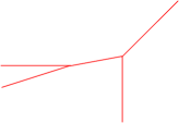
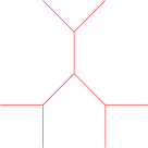
a) A tropical line in ${\mathbb{T}}^{3}$		b) A “snowflake” line in ${\mathbb{T}}^{5}$		c) A “caterpillar” line in ${\mathbb{T}}^{5}$

Figure 16. Different tropical lines

It turns out that different tropical models are related by an operation known as tropical modification. In fact, the example which we just saw with a tropical line in ${\mathbb{T}}^{2}$ along with the projection to ${\mathbb{T}}$ in the vertical direction is precisely a tropical modification of ${\mathbb{T}}$. Let us take a look at another example in two dimensions. Consider the tropical polynomial in two variables $P(x,y)=x\downY y\downY 0$ over the tropical hyperfield. The subset $\Pi$ of ${\mathbb{T}}^{3}$ defined by $z$ $\in$ $P(x,y)$ is drawn in Figure 17. It is a piecewise linear surface with $2$-dimensional faces; three of them are in the downwards vertical direction and arise due to $P(x,y)$ being multivalued. These six faces are glued along any pair of the four rays starting at $(0,0,0)$ and in the directions

$$u_{1}=(-1,0,0),\qquad u_{2}=(0,-1,0),\qquad u_{3}=(0,0,-1),\qquad\text{and}\qquad u_{0}=(1,1,1).$$

Just as in Section 5.3, we may consider the limit of amoebas $\text{Log}_{t}({\mathcal{P}})$ of the plane ${\mathcal{P}}\subset{\mathbb{R}}^{3}$ defined by the equation $x+y+z+1=0$. This limit is again the piecewise linear surface $\Pi$, and therefore this latter provides another tropical model of a classical plane! Notice that once again the projection which forgets the third coordinate establishes a bijection between ${\mathcal{P}}$ and ${\mathbb{R}}^{2}$, but is not a bijection between $\Pi$ and ${\mathbb{T}}^{2}$. This projection map $\Pi\longrightarrow{\mathbb{T}}^{2}$ is a tropical modification of the tropical plane ${\mathbb{T}}^{2}$.

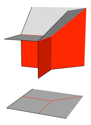
Figure 17. A modification $\Pi$ of the tropical affine plane ${\mathbb{T}}^{2}$

You might ask why one would want to use this more complicated model $\Pi$ of a plane rather than just ${\mathbb{T}}^{2}$. Let us show an example. Consider the real line,

$${\mathcal{L}}=\{(x,y)\in{\mathbb{R}}^{2}\ |\ x+y+1=0\}\subset{\mathbb{R}}^{2},$$

and let $L\subset{\mathbb{T}}^{2}$ be the corresponding tropical line, i.e. $L=\lim_{t\to+\infty}\text{Log}_{t}({\mathcal{L}})$. Let ${\mathcal{L}}^{\prime}_{t}$ be a family of lines in ${\mathbb{R}}^{2}$ whose amoebas converge to some tropical line $L^{\prime}\subset{\mathbb{T}}^{2}$ as in Theorem 5.2, and define $p_{t}={\mathcal{L}}\cap{\mathcal{L}}^{\prime}_{t}$. Now let us ask the following question: can one determine $\lim_{t\to+\infty}\text{Log}_{t}(p_{t})$ by only looking at the tropical picture?

If the set-theoretic intersection of $L$ and $L^{\prime}$ consist of a single point $p$, then $\text{Log}_{t}(p_{t})$ has no choice but to converge to $p$. But what happens when this set-theoretic intersection is infinite?

Suppose that $L^{\prime}$ is given by the tropical polynomial $``1\cdot x+y+0"$, so that the position of $L$ and $L^{\prime}$ is as in Figure 9a with $L$ in blue and $L^{\prime}$ in red. Then the stable intersection of $L$ and $L^{\prime}$ is the vertex of $L^{\prime}$, that is to say the point $(-1,0)$. Note that this is independent of the family ${\mathcal{L}}^{\prime}_{t}$, as long as $\text{Log}_{t}({\mathcal{L}}^{\prime}_{t})$ converges to $L^{\prime}$. However depending on the family ${\mathcal{L}}^{\prime}_{t}$, the point $\lim_{t\to+\infty}\text{Log}_{t}(p_{t})$ may be located anywhere on the half-line $\{(x,0),-\infty\leq x\leq-1\}$. Indeed, given the family

$${\mathcal{L}}^{\prime}_{t}=\{(x,y)\in{\mathbb{R}}^{2}\ |\ (t+1)x+y+(1-t^{b+1})=0\}\textrm{ with }b\leq-1,$$

then according to Theorem 5.2, $\lim_{t\to+\infty}\text{Log}_{t}({\mathcal{L}}^{\prime}_{t})=L^{\prime}$. Yet we have $p_{t}=(t^{b},-1-t^{b})$, and so $\lim_{t\to+\infty}\text{Log}_{t}(p_{t})=(b,0)$. Similarly, we get $\lim_{t\to+\infty}\text{Log}_{t}(p_{t})=(-\infty,0)$ by taking

$${\mathcal{L}}^{\prime}_{t}=\{(x,y)\in{\mathbb{R}}^{2}\ |\ tx+y+1=0\}.$$

This shows that using the tropical model $L,L^{\prime}\in{\mathbb{T}}^{2}$, it is impossible to extract information about the location of the intersection point of ${\mathcal{L}}$ and ${\mathcal{L}}^{\prime}_{t}$. It turns out that changing the model ${\mathbb{T}}^{2}$ via a tropical modification unveils the location of the limit of the intersection point $p_{t}$. To obtain our new model let us consider again the plane ${\mathcal{P}}\subset{\mathbb{R}}^{3}$ with equation $x+y+z+1=0$, and the projection

$$\begin{array}[]{cccc}\pi:&{\mathcal{P}}&\longrightarrow&{\mathbb{R}}^{2}\\ &(x,y,z)&\longmapsto&(x,y)\end{array}.$$

The map $\pi$ is clearly a bijection, and $\pi^{-1}(x,y)=(x,y,-x-y-1)$. The intersection of ${\mathcal{P}}$ with the plane $z=0$ in ${\mathbb{R}}^{3}$ is precisely the line ${\mathcal{L}}$. This implies that $\text{Log}_{t}(\pi^{-1}({\mathcal{L}}))\subset\{z=-\infty\}$ and

$$\lim_{t\to+\infty}\text{Log}_{t}(\pi^{-1}({\mathcal{L}}))=\Pi\cap\{z=-\infty\}\subset{\mathbb{T}}^{3}.$$

If ${\mathcal{L}}^{\prime}_{t}$ is a family of lines in ${\mathbb{R}}^{2}$ as above, then $\pi^{-1}({\mathcal{L}}^{\prime}_{t})$ is a family of lines in ${\mathcal{P}}$, and moreover the intersection point $p_{t}$ must satisfy $\pi^{-1}(p_{t})\in\{z=0\}.$ In particular we have

$$\lim_{t\to+\infty}\text{Log}_{t}(\pi^{-1}(p_{t}))\in\{z=-\infty\}.$$

Now it turns out that $L^{\prime\prime}=\lim_{t\to+\infty}\text{Log}_{t}(\pi^{-1}({\mathcal{L}}^{\prime}_{t}))$ is a tropical line in $\Pi$, which intersects the plane $\{z=-\infty\}$ in a single point! Therefore, upon projection back to ${\mathbb{R}}^{2}$ this point is nothing else but $\lim_{t\to+\infty}\text{Log}_{t}(p_{t})$, in other words the location of $\lim_{t\to+\infty}\text{Log}_{t}(p_{t})$ is now revealed by considering the tropical picture in ${\mathbb{T}}^{3}$. In Figure 18 we depict the case when ${\mathcal{L}}^{\prime}_{t}$ is given by $(t+1)x+y+(1-t^{b+1})=0$.

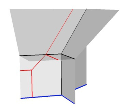
Figure 18. The tropical lines $L$ and $L^{\prime\prime}$ in the modified plane $\Pi$

Hence there is no unique or canonical choice of a tropical model of a classical space, and tropical modification is the tool used to pass between the different models. There is a single space which captures in a sense all the possible tropical models, it is known as the Berkovich space of the classical object. As one can imagine the structure of a Berkovich space is extremely complicated due to the infinitely many different tropical models. For example, the Berkovich line is an infinite tree. In a sense, a tropical model gives us just a snapshot of the complicated Berkovich space and modifications are what allow us to change the resolution.

6.3. Higher (co)dimension

In the first part of this text our main object of study was tropical curves in the plane. Even in this limited case there are many applications to classical geometry. In higher dimensions things become a bit trickier as the links between the tropical and classical worlds become more intricate.

As we mentioned earlier, definitions of Sections 1 and 2 as well as Theorem 5.2 admit natural generalisations to polynomials with any number of variables. A tropical polynomial in $n$-variables $P(x_{1},\dots,x_{n})$ defines a tropical hypersurface in ${\mathbb{T}}^{n}$, which is the corner locus of the graph of $P$ equipped with some weights. A tropical hypersurface in ${\mathbb{T}}^{n}$ is glued from flat pieces, has dimension $n-1$, satisfies a balancing condition similar to curves, and arises as the limit of amoebas of a family of complex hypersurfaces. Because of this we say that all tropical hypersurfaces are approximable.

It is also natural to consider tropical objects of dimension less than $n-1$ in ${\mathbb{T}}^{n}$. A $k$-dimensional tropical variety is a weighted polyhedral complex of dimension $k$ satisfying a generalisation of the balancing condition which we saw for curves. It would be too technical and probably useless to give here the balancing condition in full generality. Nevertheless in the case of curves, i.e. when $k=1$, the definition is the same as in Section 2.3: a tropical curve in ${\mathbb{R}}^{n}$ is a graph whose edges have a rational direction, are equipped with positive integer weights. In addition, the graph must satisfy the balancing condition given in Section 2.3 at each vertex. Unfortunately, Theorem 5.2 does not generalise to the case of higher codimensions: there exist tropical varieties, said to be not approximable, which do not arise as limits of amoebas of complex varieties of the same degree. For our purposes, we may think of a complex variety in ${\mathbb{C}}^{n}$ as being the solution set of a system of polynomial equations in $n$-variables.

Already in ${\mathbb{T}}^{3}$ there are many examples of tropical curves which are not approximable. More intricately, there are examples of pairs of tropical varieties $Y\subset X\subset{\mathbb{T}}^{n}$ for which both $Y$ and $X$ are approximable independently, however there do not exist approximations $\mathcal{Y}_{t}$ and $\mathcal{X}_{t}$ of $Y$ and $X$ with $\mathcal{Y}_{t}\subset\mathcal{X}_{t}$. Let us give an explicit example of such a pair.

Consider the modified tropical plane $\Pi\subset{\mathbb{T}}^{3}$ we just encountered, which is approximated by the amoebas of the complex plane ${\mathcal{P}}\subset{\mathbb{C}}^{3}$ defined by the equation $x+y+z+1=0$. Now, the union of three rays in the directions

$$(-2,-3,0),\qquad(0,1,1),\qquad(2,2,-1)$$

with each ray equipped with weight $1$ is a tropical curve $C\subset{\mathbb{T}}^{3}$. We may check that the balancing condition is satisfied:

$$(-2,-3,0)+(0,1,1)+(2,2,-1)=0.$$

Moreover $C$ is contained in the tropical plane $\Pi$, since we may express the three rays as

$$(-2,-3,0)=2u_{1}+3u_{2},\qquad(0,1,1)=u_{0}+u_{1},\qquad(2,2,-1)=2u_{0}+3u_{3},$$

where the $u_{i}$ are the directions of the rays of $\Pi$ given in Section 6.2. The tropical curve $C$ is approximable, however there are no approximations ${\mathcal{C}}_{t}$ and ${\mathcal{P}}_{t}$ of $C$ and $\Pi$ with ${\mathcal{C}}_{t}\subset{\mathcal{P}}_{t}$. The full proof of this statement involves several steps, and we only focus here on the essential one. Hence let us assume that we may take both families ${\mathcal{P}}_{t}$ and ${\mathcal{C}}_{t}$ to be constant, with ${\mathcal{P}}_{t}$ equal to the above plane ${\mathcal{P}}$ for all $t$. That is to say we are reduced to showing that there does not exist a complex curve ${\mathcal{C}}\subset{\mathcal{P}}$ such that $C=\lim_{t\to+\infty}\text{Log}_{t}({\mathcal{C}})$.

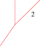
Figure 19. The projection of the curve $C\subset P$ to ${\mathbb{T}}^{2}$ along with its dual polygon

Suppose on the contrary that such a complex curve ${\mathcal{C}}$ exists. The projection of $C$ to ${\mathbb{T}}^{2}$ which forgets the $z$-coordinate is a tropical curve $C^{\prime}$ as defined in Section 2. The curve $C^{\prime}$ and its Newton polygon are shown in Figure 19. A polynomial with such a Newton polygon is of degree $3$ and has the form $P(x,y)=ax^{3}+by^{2}+\dots$, where the monomials after the dots have higher degree. A complex curve in ${\mathbb{C}}^{2}$ with such an equation has a type of singularity at $(0,0)$ known as a cusp. Hence the ray of $C$ in the direction $(-2,-3,0)=2u_{1}+3u_{2}$ tells us that the projection of ${\mathcal{C}}$ has a cusp at $(0,0)$. Since ${\mathcal{C}}$ is contained in ${\mathcal{P}}$ and ${\mathcal{P}}$ projects bijectively to ${\mathbb{C}}^{2}$, we deduce that ${\mathcal{C}}$ itself has a cusp at $(0,0,-1)$. In a similar way, the ray in direction $2u_{0}+3u_{3}$ implies that ${\mathcal{C}}$ must have a second cusp at infinity. However it is known that a plane curve of degree $3$ can have at most one cusp, which contradicts the existence of ${\mathcal{C}}$. This tells us that our tropical curve is not approximable by a complex algebraic curve of degree $3$ contained in the plane ${\mathcal{P}}$.

Many other examples of non-approximable tropical objects exist, including lines in surfaces, curves in space, and even linear spaces. What must be stressed is that from a purely combinatorial view point it is very difficult to distinguish these pathological tropical objects from approximable ones. This is just one of the problems that makes tropical geometry continue to be a challenging and exciting field of research especially in terms of its relations to classical geometry.

7. References

The references given below contain the proofs of statements contained throughout the text. They also present the many directions in which tropical geometry is developing. The references to the literature go far beyond what we mention here; it would be impossible to provide a complete list. However, we hope to give an account of the multitude of perspectives on tropical geometry.

Firstly, we should note that tropical curves first appeared under the name of $(p,q)$-webs, in the work of the physicists O. Aharony, A. Hanany, and B. Kol [AHK98]. In mathematics, roots of tropical geometry can be traced back, at least to the work of Bergman [Ber71] on logarithmic limit sets of algebraic varieties, of Bieri and Groves [BG84] on non-archimedean valuations, of Viro on patchworking (see references below), as well to the study of toric varieties, which provide a first relation between convex polytopes and algebraic geometry, see for example [Ful93], [DK86].

There are other general introductions to tropical geometry. The texts [BPS08] and [SS09] are aimed at the interested reader with a minimal background in mathematics, similar to the one assumed in this text. There the authors emphasize different applications of tropical geometry, enumerative geometry in [BPS08], and phylogenetics in [SS09]. More confident readers can also read the works of [RGST05], [Gat06], [IMS07], [Mik07], [IM12], [Mac12], [MS], and [MR]. For established geometers, we recommend the state of the art [Mik04] and [Mik06].

In particular stable intersections of tropical curves in ${\mathbb{R}}^{2}$ are discussed in detail in [RGST05]. The proof of Bézout Theorem we gave is contained in [Gat06]. Foundations of a more sophisticated tropical intersection theory are exposed in [Mik06], and further developed in [AR10], [Kat09], [Sha13].

Amoebas of algebraic varieties were introduced in [GKZ94]. The interested reader can also see the texts [Pas08], [Vir02], and the more sophisticated [PR04]. For a deeper look at patchworking, amoebas, and Maslov’s dequantisation, as well as their applications to Hilbert’s 16th problem we point you to the texts, [Vir01], [Vir08], [Mik04] and [Mik00] as well as the website [Vira]. We especially recommend the text [IV96], dedicated to a large audience, which explains how patchworking has been used to disprove the Ragsdale conjecture which has been open for decades.

For more on tropical hyperfields we point the reader towards [Virb]. As we mentioned in the text, there are other enrichments of the tropical semi-field, some examples can be found in [IR10], [DW11] and [CC]. Tropical modifications were introduced by Mikhalkin in the above mentioned text [Mik06], and their relations to Berkovich spaces can be found in [Pay09] and [Pay]. This perspective from Berkovich spaces allows one to relate tropical geometry to algebraic geometry not only over ${\mathbb{C}}$ but over any field equipped with a so-called non-archimedean valuation (e.g. the $p$-adic numbers equipped with the $p$-adic valuation). For this point of view, we refer for example to [Rab12], [BPR], [ACP] and reference therein. The approximation problem has been studied mostly in the case of curves. For tropical curves see [Mik05], [Mik06], [Spe], [NS06], [Nis], [Tyo12], [Kat12], [ABBR]. For a look at the approximation problem of curves in surfaces as in the example provided in the last section, see [BK12], [BS], and [GSW]. Among all sources of motivation to study the latter problem, we refer to the very nice study of tropical lines in tropical surfaces in ${\mathbb{R}}^{3}$ by Vigeland in [Vig09] and [Vig].

To end this introduction to tropical geometry, we want to point out that this subject has very successful applications to many fields other than Hilbert’s 16th problem, such as enumerative geometry [Mik05], algebraic geometry [Tev07], mirror symmetry [Gro11], mathematical biology [AK06], [PS05], computational complexity [AGG12] computational geometry [STY07], [CTY10], and algebraic statistics [CMS10], [PS05] just to name a few…

References

- [ABBR] O. Amini, M. Baker, E. Brugallé, and J. Rabinoff. Lifting harmonic morphisms of tropical curves, metrized complexes, and Berkovich skeleta. arXiv:1303.4812.
- [ACP] D. Abramovich, L. Caporaso, and S. Payne. The tropicalization of the moduli space of curves. arXiv:1212.0373.
- [AGG12] M. Akian, S. Gaubert, and A. Guterman. Tropical polyhedra are equivalent to mean payoff games. Internat. J. Algebra Comput., 22(1):1250001, 43, 2012.
- [AHK98] O. Aharony, A. Hanany, and B. Kol. Webs of (p,q) 5-branes, five dimensional field theories and grid diagrams. J High Energy Phys, 1(2), 1998.
- [AK06] F. Ardila and C.J. Klivans. The Bergman complex of a matroid and phylogenetic trees. J. Comb. Theory Ser. B, 96(1):38–49, 2006.
- [AR10] L. Allermann and J. Rau. First steps in tropical intersection theory. Mathematische Zeitschrift, 264:633–670, 2010.
- [Ber71] G. M. Bergman. The logarithmic limit-set of an algebraic variety. Trans. Amer. Math. Soc., 157:459–469, 1971.
- [BG84] R. Bieri and J. Groves. The geometry of the set of characters induced by valuations. J. Reine Angew. Math., 347:168–195, 1984.
- [BK12] T. Bogart and E. Katz. Obstructions to lifting tropical curves in surfaces in 3-space. SIAM J. Discrete Math., 26(3):1050–1067, 2012.
- [BPR] M. Baker, S. Payne, and J. Rabinoff. Nonarchimedean geometry, tropicalization, and metrics on curves. arXiv:1104.0320.
- [BPS08] N. Berline, A. Plagne, and C. Sabbah, editors. Géométrie tropicale. Éditions de l’École Polytechnique, Palaiseau, 2008.
- [Bru09] E. Brugallé. Un peu de géométrie tropicale. Quadrature, (74):10–22, 2009.
- [BS] E. Brugallé and K. Shaw. Obstructions to approximating tropical curves in surfaces via intersection theory. arXiv:1110.0533.
- [CC] A. Connes and C. Consani. The universal thickening of the field of real numbers. arXiv:1202.4377.
- [CMS10] M. A. Cueto, J. Morton, and B. Sturmfels. Geometry of the restricted Boltzmann machine. In Algebraic methods in statistics and probability II, volume 516 of Contemp. Math., pages 135–153. Amer. Math. Soc., Providence, RI, 2010.
- [CTY10] M. A. Cueto, E. A. Tobis, and J. Yu. An implicitization challenge for binary factor analysis. J. Symbolic Comput., 45(12):1296–1315, 2010.
- [DK86] V. I. Danilov and A. G. Khovanskiĭ. Newton polyhedra and an algorithm for calculating Hodge-Deligne numbers. Izv. Akad. Nauk SSSR Ser. Mat., 50(5):925–945, 1986.
- [DW11] A. Dress and W. Wenzel. Algebraic, tropical, and fuzzy geometry. Beitr. Algebra Geom., 52(2):431–461, 2011.
- [Ful93] W. Fulton. Introduction to toric varieties, volume 131 of Ann. Math. Studies. Princeton Univ. Press., 1993.
- [Gat06] A. Gathmann. Tropical algebraic geometry. Jahresber. Deutsch. Math.-Verein., 108(1):3–32, 2006.
- [GKZ94] I. M. Gelfand, M. M. Kapranov, and A. V. Zelevinsky. Discriminants, resultants, and multidimensional determinants. Mathematics: Theory & Applications. Birkhäuser Boston Inc., Boston, MA, 1994.
- [Gro11] M. Gross. Tropical geometry and mirror symmetry, volume 114 of CBMS Regional Conference Series in Mathematics. Published for the Conference Board of the Mathematical Sciences, Washington, DC, 2011.
- [GSW] A. Gathmann, K. Schmitz, and A. Winstel. The realizability of curves in a tropical plane. arXiv:1307.5686.
- [IM12] I. Itenberg and G. Mikhalkin. Geometry in the tropical limit. Math. Semesterber., 59(1):57–73, 2012.
- [IMS07] I. Itenberg, G Mikhalkin, and E. Shustin. Tropical Algebraic Geometry, volume 35 of Oberwolfach Seminars Series. Birkhäuser, 2007.
- [IR10] Z. Izhakian and L. Rowen. A guide to supertropical algebra. In Advances in ring theory, Trends Math., pages 283–302. Birkhäuser/Springer Basel AG, Basel, 2010.
- [IV96] I. Itenberg and O. Viro. Patchworking algebraic curves disproves the Ragsdale conjecture. Math. Intelligencer, 18(4):19–28, 1996.
- [Kat09] E. Katz. A tropical toolkit. Expo. Math., 2009.
- [Kat12] E. Katz. Lifting tropical curves in space and linear systems on graphs. Adv. Math., 230(3):853–875, 2012.
- [Mac12] D. Maclagan. Introduction to tropical algebraic geometry. In Tropical geometry and integrable systems, volume 580 of Contemp. Math., pages 1–19. Amer. Math. Soc., Providence, RI, 2012.
- [Mik00] G. Mikhalkin. Real algebraic curves, the moment map and amoebas. Ann. of Math. (2), 151(1):309–326, 2000.
- [Mik04] G. Mikhalkin. Amoebas of algebraic varieties and tropical geometry. In Different faces of geometry, volume 3 of Int. Math. Ser. (N. Y.), pages 257–300. Kluwer/Plenum, New York, 2004.
- [Mik05] G. Mikhalkin. Enumerative tropical algebraic geometry in . J. Amer. Math. Soc., 18(2):313–377, 2005.
- [Mik06] G. Mikhalkin. Tropical geometry and its applications. In International Congress of Mathematicians. Vol. II, pages 827–852. Eur. Math. Soc., Zürich, 2006.
- [Mik07] G. Mikhalkin. What isa tropical curve? Notices Amer. Math. Soc., 54(4):511–513, 2007.
- [MR] G. Mikhalkin and J. Rau. Tropical geometry. Book in progress, draft available at https://www.dropbox.com/s/g3ehtsoyy3tzkki/main.pdf.
- [MS] D. Maclagan and B. Sturmfels. Introduction to tropical geometry. Book in progress, draft available at http://homepages.warwick.ac.uk/staff/D.Maclagan/papers/papers.html.
- [Nis] T. Nishinou. Correspondence theorems for tropical curves. arXiv:0912.5090.
- [NS06] T. Nishinou and B. Siebert. Toric degenerations of toric varieties and tropical curves. Duke Math. J., 135(1):1–51, 2006.
- [Pas08] M. Passare. How to compute by solving triangles. Amer. Math. Monthly, 115:745–752, 2008.
- [Pay] S. Payne. Topology of nonarchimedean analytic spaces and relations to complex algebraic geometry. arXiv:1309.4403.
- [Pay09] S. Payne. Analytification is the limit of all tropicalizations. Math. Res. Lett., 16(3):543–556, 2009.
- [PR04] M. Passare and H. Rullgård. Amoebas, Monge-Ampère measures, and triangulations of the Newton polytope. Duke Math. J., 121(3):481–507, 2004.
- [PS05] L. Pachter and B. Sturmfels. Biology. In Algebraic statistics for computational biology, pages 125–159. Cambridge Univ. Press, New York, 2005.
- [Rab12] J. Rabinoff. Tropical analytic geometry, Newton polygons, and tropical intersections. Adv. Math., 229:3192–3255, 2012.
- [RGST05] J. Richter-Gebert, B. Sturmfels, and T. Theobald. First steps in tropical geometry. In Idempotent mathematics and mathematical physics, volume 377 of Contemp. Math., pages 289–317. Amer. Math. Soc., Providence, RI, 2005.
- [Sha13] K. Shaw. A tropical intersection product in matroidal fans. SIAM J. Discrete Math., 27(1):459–491, 2013.
- [Spe] D. Speyer. Uniformizing tropical curves I: Genus zero and one. arXiv: 0711.2677.
- [SS09] D. Speyer and B. Sturmfels. Tropical mathematics. Math. Mag., 82(3):163–173, 2009.
- [STY07] B. Sturmfels, J. Tevelev, and J. Yu. The Newton polytope of the implicit equation. Mosc. Math. J., 7(2):327–346, 2007.
- [Tev07] J. Tevelev. Compactifications of subvarieties of tori. Amer. J. Math., 129(4):1087–1104, 2007.
- [Tyo12] I. Tyomkin. Tropical geometry and correspondence theorems via toric stacks. Math. Ann., 353(3):945–995, 2012.
- [Vig] M. D. Vigeland. Tropical lines on smooth tropical surfaces. arXiv:0708.3847.
- [Vig09] M. D. Vigeland. Smooth tropical surfaces with infinitely many tropical lines. Arkiv för Matematik, 48(1):177–206, 2009.
- [Vira] O. Viro. https://www.math.sunysb.edu/ oleg/patchworking.html.
- [Virb] O. Viro. Hyperfields for tropical geometry i. hyperfields and dequantization. arXiv:1006.3034.
- [Vir01] O. Viro. Dequantization of real algebraic geometry on logarithmic paper. In European Congress of Mathematics, Vol. I (Barcelona, 2000), volume 201 of Progr. Math., pages 135–146. Birkhäuser, Basel, 2001.
- [Vir02] O. Viro. What is an amoeba? Notices of the AMS, 49:916–917, 2002.
- [Vir08] O. Viro. From the sixteenth Hilbert problem to tropical geometry. Japanese Journal of Mathematics, 3(2):185–214, 2008.