3cm2cm2cm2cm
Local solvability and turning for the inhomogeneous Muskat problem
Abstract
In this work we study the evolution of the free boundary between two different fluids in a porous medium where the permeability is a two dimensional step function. The medium can fill the whole plane or a bounded strip . The system is in the stable regime if the denser fluid is below the lighter one. First, we show local existence in Sobolev spaces by means of energy method when the system is in the stable regime. Then we prove the existence of curves such that they start in the stable regime and in finite time they reach the unstable one. This change of regime (turning) was first proven in [5] for the homogeneus Muskat problem with infinite depth.
Keywords: Darcy’s law, inhomogeneous Muskat problem, well-posedness, blow-up, maximum principle.
Acknowledgments: The authors are supported by the Grants MTM2011-26696 and SEV-2011-0087 from Ministerio de Ciencia e Innovación (MICINN). Diego Córdoba was partially supported by StG-203138CDSIF of the ERC. Rafael Granero-Belinchón is grateful to Department of Applied Mathematics ”Ulisse Dini” of the Pisa University for the hospitality during May-July 2012. We are grateful to Instituto de Ciencias Matemáticas (Madrid) and to the Dipartimento di Ingegneria Aerospaziale (Pisa) for computing facilities.
1 Introduction
In this work we study the evolution of the interface between two different incompressible fluids with the same viscosity coefficient in a porous medium with two different permeabilities. This problem is of practical importance because it is used as a model for a geothermal reservoir (see [6] and references therein). The velocity of a fluid flowing in a porous medium satisfies Darcy’s law (see [3, 23, 24])
| (1) |
where is the dynamic viscosity, is the permeability of the medium, is the acceleration due to gravity, is the density of the fluid, is the pressure of the fluid and is the incompressible velocity field. In our favourite units, we can assume
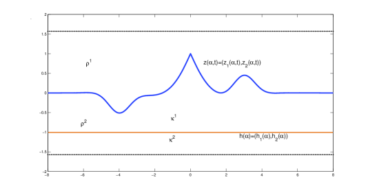
The spatial domains considered in this work are (infinite depth) and (finite depth). We have two immiscible and incompressible fluids with the same viscosity and different densities; fill in the upper domain and fill in the lower domain . The curve
is the interface between the fluids. In particular we are making the ansatz that and are a partition of and they are separated by a curve .
The system is in the stable regime if the denser fluid is below the lighter one, i.e. . This is known in the literature as the Rayleigh-Taylor condition. The function that measures this condition is defined as
In the case with , the motion of a fluid in a two-dimensional porous medium is analogous to the Hele-Shaw cell problem (see [7, 9, 17, 19] and the references therein) and if the fluids fill the whole plane (in the case with the same viscosity but different densities) the contour equation satisfies (see [11])
| (2) |
They show the existence of classical solution locally in time (see [11] and also [1, 15, 16, 20]) in the Rayleigh-Taylor stable regime which means that , and maximum principles for and (see [12]). Moreover, in [5] the authors show that there exists initial data in such that blows up in finite time. Furthermore, in [4] the authors prove that there exist analytic initial data in the stable regime for the Muskat problem such that the solution turns to the unstable regime and later no longer belongs to . In [8] the authors show an energy balance for and that if initially , then there is global lipschitz solution and if the initial datum has then there is global classical solution. In [10, 27] the authors study the case with different viscosities. In [21] the authors study the case where the interface reach the boundary in a moving point with a constant (non-zero) angle.
The case where the fluid domain is the strip , with , has been studied in [14, 15, 16]. In this regime the equation for the interface is
| (3) |
For equation (3) the authors in [14] obtain the existence of classical solution locally in time in the stable regime case where the initial interface does not reach the boundaries, and the existence of finite time singularities. These singularities mean that the curve is initially a graph in the stable regime, and in finite time, the curve can not be parametrized as a graph and the interface turns to the unstable regime. Also the authors study the effect of the boundaries on the evolution of the interface, obtaining the maximum principle and a decay estimate for and the maximum principle for for initial datum satisfying smallness conditions on and on . So, not only the slope must be small, also amplitude of the curve plays a role. Both result differs from the results corresponding to the infinite depth case (2). We note that the case with boundaries can also be understood as a problem with different permeabilities where the permeability outside vanishes. In the forthcoming work [18] the authors compare the different models (2), (3) and (6) from the point of view of the existence of turning waves.
In this work we study the case where permeability is a step function, more precisely, we have a curve
separating two regions with different values for the permeability (see Figure 1). We study the regime with infinite depth, for periodic and for ”flat at infinity” initial datum, but also the case where the depth is finite and equal to . In the region above the curve the permeability is , while in the region below the curve the permeability is . Note that the curve is known and fixed. Then it follows from Darcy’s law that the vorticity is
where corresponds to the difference of the densities, corresponding to the difference of permeabilities and is the usual Dirac’s distribution. In fact both amplitudes for the vorticity are quite different, while is a derivative, the amplitude has a nonlocal character (see (5), (7) and Section 2). The equation for the interface, when and the fluid fill the whole plane, is
| (4) |
with
| (5) |
If the fluids fill the whole space but the initial curve is periodic the equation reduces to
| (6) |
where the second vorticity amplitude can be written as
| (7) |
If we consider the regime where the amplitude of the wave and the depth of the medium are of the same order then the equation for the interface, when the depth is chosen to be , is
| (8) | |||||
where
| (9) | |||||
with
a Schwartz function.
Remark 1 For notational simplicity, we denote and we drop the dependence.
The plan of the paper is as follows: in Section 2 we derive the contour equations (4),(6) and (8). In Section 3 we show the local in time solvability and an energy balance for the norm. In Section 4 we perform numerics and in Section 5 we obtain finite time singularities for equations (4) (6) and (8) when the physical parameters are in some region and numerical evidence showing that, in fact, every value is valid for the physical parameters.
2 The contour equation
In this section we derive the contour equations (4), (6) and (8), i.e. the equations for the interface. First we obtain the equation in the infinite depth case, both, flat at infinity and periodic. Given a scalar, curves, and a spatial domain or , we denote the Birkhoff-Rott integral as
| (10) |
where denotes the kernel of (which depends on the domain). If the domain is we have
| (11) |
for we have
| (12) |
and for the kernel is (see [14])
| (13) |
2.1 Infinite depth
2.1.1 Assuming :
We have
| (15) |
and
| (16) |
We observe that is the limit inside (the upper subdomain) and is the limit inside (the lower subdomain). The curve doesn’t touch the curve , so, the limit for the curve are in the same domain .
Using Darcy’s Law and assuming that the initial interface is in the region with permeability , we obtain
where in the last equality we have used the continuity of the pressure along the interface (see [10]). Using (15) we conclude
| (17) |
We need to determine . We consider
where the first equality is due to Darcy’s Law. Using the expression (16) we have
| (18) |
We take , with a fixed constant. Then
where denotes the Hilbert transform. Finally, we have
| (19) |
(see Remark 1 for the definition of ). The identity
gives us
and
Thus,
| (20) |
and
Due to the conservation of mass the curve is advected by the flow, but we can add any tangential term in the equation for the evolution of the interface without changing the shape of the resulting curve (see [10]), i.e. we consider that the equation for the curve is
Taking , we conclude
| (21) |
By choosing this tangential term, if our initial datum can be parametrized as a graph, we have Therefore the parametrization as a graph propagates.
Finally we conclude (4) as the evolution equation for the interface (which initially is a graph above the line ). We remark that the second vorticity (5) can be written in equivalent ways
| (22) | |||||
Remark 2 Notice that in the case with different viscosities the expression for the amplitude of the vorticity located at the interface (see equation (17)) is no longer valid. Instead, we have
To this integral equation, we add the equation (18) or (20). Thus, one needs to invert an operator. This is a rather delicate issue that is beyond the scope of this paper (see [10] for further details in the case ).
2.1.2 Assuming :
We have that (14) is still valid, but now are periodic functions and . Using complex variables notation we have
Changing variables and using the identity
we obtain
Equivalently,
Recall that (17) and (20) are still valid if for a fixed constant. We have
thus, the velocity in the curve when the correct tangential terms are added is
| (24) |
We can do the same in order to write as an integral on the torus.
| (25) |
If the initial datum can be parametrized as a graph the equation for the interface reduces to (6), where the second vorticity amplitude (7) can be written as
| (26) | |||||
| (27) |
2.2 Finite depth
Now we consider the bounded porous medium (see Figure 1). This regime is equivalent to the case with more than two because the boundaries can be understood as regions with . As before,
We assume that with . We have that is given by (17). The main difference between the finite depth and the infinite depth is at the level of . As in the infinite depth case we have
where now has the usual definition (10) in terms of in expression (13). In the unbounded case we have an explicit expression for (20) in terms of and , but now we have a Fredholm integral equation of second kind:
| (28) |
After taking the Fourier transform, denoted by , and using some of its basic properties, we have
We can solve the equation for for any with
| (29) |
We obtain
| (30) |
Now we observe that if is a function in the Schwartz class, , such that we have that
and we obtain
Recall here that in order to obtain we invert an integral operator. In general this is a delicate issue (compare with [10]), but with our choice of this point can be addressed in a simpler way. Using
and adding the correct tangential term, we obtain
| (31) | |||||
If the initial curve can be parametrized as a graph the equation reduces to (8) where is defined in (9).
Remark 3 If by an explicit computation we obtain , thus, any is valid. Moreover, we have tested numerically that the same remains valid for any , so (9) would be correct for any .
3 Well-posedness in Sobolev spaces
3.1 Energy balance for the norm
Here we obtain an energy balance inequality for the norm of the solution of equation (8). We define , and .
Lemma 1.
For every the smooth solutions of (8) in the stable regime, i.e. , case verifies
| (32) |
Proof.
We define the potentials
We have in each subdomain . Since the velocity is incompressible we have
Moreover, the normal component of the velocity is continuous through the interface and the line where permeability changes . Using the impermeable boundary conditions, we only need to integrate over the curve and . Indeed, we have
| (33) |
| (34) |
| (35) |
| (36) |
Thus, summing (36) and (33) together and using the continuity of the pressure and the velocity in the normal direction, we obtain
| (37) |
Integrating in time we get the desired result (32). ∎
3.2 Well-posedness for the infinite depth case
Let be the spatial domain considered, i.e. or . In this section we prove the short time existence of classical solution for both spatial domains. We have the following result:
Theorem 1.
Consider a fixed constant and the initial datum , , such that . Then, if the Rayleigh-Taylor condition is satisfied, i.e. , there exists an unique classical solution of (4) where . Moreover, we have
Proof.
We prove the result in the case , being the case similar. Let us consider the usual Sobolev space endowed with the norm
where . Define the energy
| (38) |
with
| (39) |
To use the classical energy method we need a priori estimates. To simplify notation we drop the physical parameters present in the problem by considering and . The sign of the difference between the permeabilities will not be important to obtain local existence. We denote a constant that can changes from one line to another.
Estimates on : Given such that we consider as defined in (22). Then we have that for some constants .
We proceed now to prove this claim. We start with the norm. Changing variables in (22) we have
The inner term, can be bounded as follows
In the last inequality we have used Cauchy-Schwartz inequality and Tonelli’s Theorem. For the outer part we have
where we have used that and Cauchy-Schwartz inequality. We change variables in (2.1.1) to obtain
Now it is clear that is at the level of in terms of regularity and the inequality follows using the same techniques. Using Sobolev embedding we conclude this step.
Estimates on : The first integral in (4) can be bounded as follows
for some positive and finite . The new term is the second integral in (4).
Easily we have
We split
where denotes the Hilbert transform. Now we conclude the desired bound using the previous estimate on and Sobolev embedding. The second term can be bounded as
We obtain the following useful estimate
| (40) |
We have
Thus, integrating in time and using (40),
and we conclude this step
Estimates on : As before, the bound for the term coming from the first integral in (4) can be obtained as in [11], so it only remains the term coming from the second integral. We have
For the sake of brevity we only bound the terms with higher order, being the remaining terms analogous. We have
with
and
In order to bound we use the symmetries in the formulae () and we integrate by parts:
In we use Cauchy-Schwartz inequality to obtain
The bounds for and are similar:
Finally, we integrate by parts in and we get
As a conclusion, we obtain
Putting all the estimates together we get the desired bound for the energy:
| (41) |
Regularization: This step is classical, so, we only sketch this part (see [22] for the details). We regularize the problem and we show that the regularized problems have a solution using Picard’s Theorem on a ball in . Using the previous energy estimates and the fact that the initial energy is finite, these solutions have the same time of existence ( depending only on the initial datum) and we can show that they are a Cauchy sequence in . From here we obtain where and , a solution to (4) as the limit of these regularized solutions. The continuity of the strongest norm for positive times follows from the parabolic character of the equation. The continuity of at follows from the fact that in and from the energy estimates.
Uniqueness: Only remains to show that the solution is unique. Let us suppose that for the same initial datum there are two smooth solutions and with finite energy as defined in (38) and consider . Following the same ideas as in the energy estimates we obtain
Now we conclude using Gronwall inequality. ∎
3.3 Well-posedness for the finite depth case
In this section we prove the short time existence of classical solution in the case where the depth is finite. We have the following result:
Theorem 2.
Consider a constant and , , an initial datum such that and . Then, if the Rayleigh-Taylor condition is satisfied, i.e. , there exists an unique classical solution of (8) where . Moreover, we have
Proof.
Let us consider the usual Sobolev space , being the other cases analogous, and define the energy
| (42) |
with
| (43) |
and
| (44) |
We note that represents the distance between and and the distance between and the boundaries. To simplify notation we drop the physical parameters present in the problem by considering and . Again, the sign of the difference between the permeabilities will not be important to obtain local existence. We write (8) as , being the integrals corresponding and the integrals involving . We denote a constant that can changes from one line to another.
Estimate on : Given such that and consider as defined in (9). Then we have that . We need to bound and with
We have
where we have used Tonelli’s Theorem and Cauchy-Schwartz inequality. Recall that , thus
and the kernel corresponding to can not be singular and we also obtain
Now, as , we can use the Young’s inequality for the convolution terms obtaining bounds with an universal constant depending on and . Indeed, we have
and we obtain
Now we observe that
and we obtain . Using Young inequality we conclude
Estimates on and : The integrals corresponding to in (8) can be bounded (see [14]) as
The new terms are the integrals and , those involving in (8). We have, when splitted accordingly to the decay at infinity,
where
and
We conclude the following useful estimate
| (45) |
We have
Thus, using (45) and integrating in time, we obtain the desired bound for :
To obtain the corresponding bound for we proceed in the same way and we use (45) (see [14] for the details)
Estimates on : As before, see [14] for the details concerning the terms coming from in (8). It only remains the terms coming from :
We split
The lower order terms (l.o.t.) can be obtained in a similar way, so we only study the terms . We have
The term is given by
Integrating by parts
Regularization and uniqueness: These steps follow the same lines as in Theorem 1. This concludes the result. ∎
4 Numerical simulations
In this section we perform numerical simulations to better understand the role of . We consider equation (6) where , and . For each initial datum we approximate the solution of (6) corresponding to different . Indeed, we take different to get and .
To perform the simulations we follow the ideas in [13]. The interface is approximated using cubic splines with spatial nodes. The spatial operator is approximated with Lobatto quadrature (using the function quadl in Matlab). Then, three different integrals appear for a fixed node . The integral between and , the integral between and and the nonsingular ones. In the two first integrals we use Taylor theorem to remove the zeros present in the integrand. In the nonsingular integrals the integrand is made explicit using the splines. We use a classical explicit Runge-Kutta method of order 4 to integrate in time. In the simulations we take and .
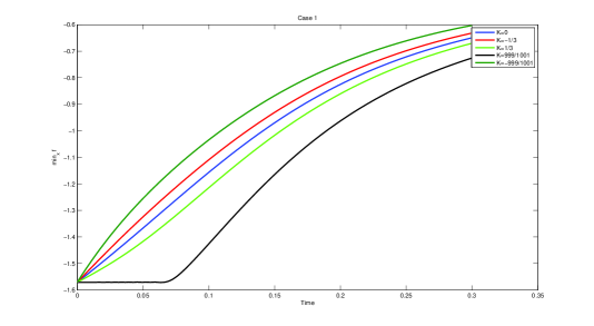
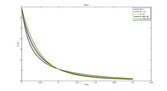
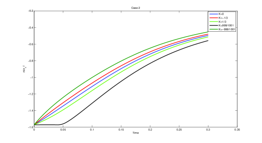
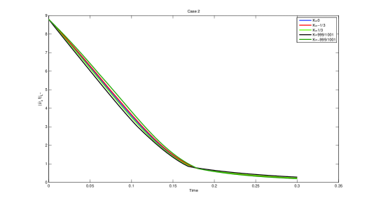
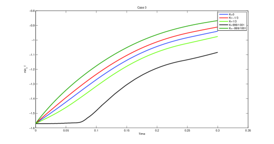
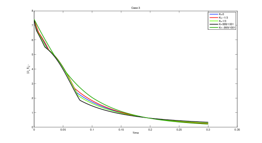
In these simulations we observe that decays but rather differently depending on . If the decay of is faster when compared with the case . In the case where the term corresponding to slows down the decay of but we observe still a decay. Particularly, we observe that if () the decay is initially almost zero and then slowly increases. When the evolution of is considered the situation is reversed. Now the simulations corresponding to have the faster decay. With these result we can not define a stable regime for in which the evolution would be smoother. Recall that we know that there is not any hypothesis on the sign or size of to ensure the existence (see Theorem 1 and 2).
5 Turning waves
In this section we prove finite time singularities for equations (4), (6) and (8). These singularities mean that the curve turns over or, equivalently, in finite time they can not be parametrized as graphs. The proof of turning waves follows the steps and ideas in [5] for the homogeneus infinitely deep case where here we have to deal with the difficulties coming from the boundaries and the delta coming from the jump in the permeabilities.
5.1 Infinite depth
Let be the spatial domain considered, i.e. or . We have
Theorem 3.
Let us suppose that the Rayleigh-Taylor condition is satisfied, i.e. . Then there exists , an admissible (see Theorem 1) initial datum, such that, for any possible choice of and , there exists a solution of (4) and (6) for which in finite time . For short time the solution can be continued but it is not a graph.
Proof.
To simplify notation we drop the physical parameters present in the problem by considering . The proof has three steps. First we consider solutions which are arbitrary curves (not necesary graphs) and we translate the singularity formation to the fact . The second step is to construct a family of curves such that this expression is negative. Thus, we have that if there exists, forward and backward in time, a solution in the Rayleigh-Taylor stable case corresponding to initial data which are arbitrary curves then, we have proved that there is a singularity in finite time. The last step is to prove, using a Cauchy-Kovalevsky theorem, that there exists local in time solutions in this unstable case.
Obtaining the correct expression: Consider the case . Due to (21) we have
where
Assume now that the following conditions for holds:
-
•
are odd functions,
-
•
, and ,
-
•
.
The previous hypotheses mean that is a curve satisfying the arc-chord condition and only has vertical component. Due to these conditions on we have and is odd (and then the second derivative at zero is zero) and we get that . For we get
We integrate by parts and we obtain, after some lengthy computations,
| (46) |
For the term with the second vorticity we have
and, after an integration by parts we obtain
| (47) |
Putting all together we obtain that in the flat at infinity case the important quantity for the singularity is
| (48) |
where, due to (20), is defined as
| (49) |
We apply the same procedure to equation (24) and we get the importat quantity in the periodic setting (recall the superscript in the notation denoting that we are in the periodic setting):
| (50) |
and, due to (25),
| (51) |
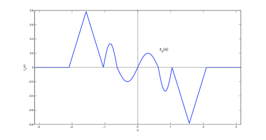
Taking the appropriate curve: To clarify the proof, let us consider first the periodic setting. Given , we consider constants such that and let us define
and
| (52) |
Due to the definition of , we have
and using (51), we get
Inserting this curve in (50) we obtain
with
and is the integral involving the second vorticity . We remark that does not depend on . The sign of is the same as the sign of , thus we get and this is independent of the choice of and . Now we fix and we take sufficiently large such that
We can do that because
or, equivalently,
if is large enough. The integral is well defined and positive, but goes to zero as grows. Then, fixed and in such a way , we take sufficiently large such that . We are done with the periodic case.
We proceed with the flat at infinity case. We take as before and and define
| (53) |
and
| (54) |
We have
and we assume . Inserting the curve (53) and (54) in (49) and changing variables, we obtain
We split the integral in two parts:
and
We have
and using that is such that , we get
The remaining integral is
and using that is such that , we get
Putting all together we get
and
Using this bound in (48) we get
Then, as before,
where are the integrals on the intervals and , respectively. We have
thus,
To ensure that the decay of is faster than the decay of we take . Now, fixing , we can obtain and such that and . Taking we obtain a curve such that . In order to conclude the argument it is enough to approximate these curves (52) and (54) by analytic functions. We are done with this step of the proof.
Showing the forward and backward solvability: At this point, we need to prove that there is a solution forward and backward in time corresponding to these curves (52) and (54). Indeed, if this solution exists then, due to the previous step, we obtain that, for a short time , the solution is a graph with finite energy (in fact, it is analytic). This graph at time has a blow up for and, for a short time , the solution can not be parametrized as a graph. We show the result corresponding to the flat at infinity case, being the periodic one analogous. We consider curves satisfying the arc-chord condition and such that
We define the complex strip and the spaces
| (55) |
with norm
where denotes the Hardy-Sobolev space on the strip with the norm
| (56) |
(see [2]). These spaces form a Banach scale. For notational convenience we write , . Recall that, for ,
| (57) |
We consider the complex extension of (20) and (21), which is given by
| (58) |
with
| (59) |
Recall the fact that in the case of a real variable graph has the same regularity as , but in the case of an arbitrary curve is, roughly speaking, at the level of the first derivative of the interface. This fact will be used below. We define
| (60) |
| (61) |
The function is the complex extension of the arc chord condition and we need it to bound the terms with . The function comes from the different permeabilities and we use it to bound the terms with . We observe that both are bounded functions for the considered curves. Consider and the set
where and are defined in (60) and (61). Then we claim that, for , the righthand side of (58), is continuous and the following inequalities holds:
| (62) | |||
| (63) | |||
| (64) |
The claim for the spatial operator corresponding to has been studied in [5], thus, we only deal with the new terms containing . For the sake of brevity we only bound some terms, being the other analogous. Using Tonelli’s theorem and Cauchy-Schwartz inequality we have that
Moreover, we get
| (65) |
For the procedure is similar but we lose one derivative. Using (57) and Sobolev embedding we conclude
| (66) |
From here inequality (62) follows. Inequality (63), for the terms involving , can be obtained using the properties of the Hilbert transform as in [5]. Let’s change slightly the notation and write for the integral in (59). We split
In we need some extra decay at infinity to ensure the finiteness of the integral. We compute
and, due to Sobolev embedding, we get
For the second term we obtain the same bound
We split componentwise. In the first coordinate we have
In the second coordinate we need to ensure the integrability at infinity. We get
and, with this splitting and the properties of the Hilbert transform, we obtain
We get
where
and
From these expressions we obtain
and
Collecting all these estimates, and due to Sobolev embedding and (57) we obtain
We are done with (63). Inequality (64) is equivalent to the bound . Such a bound for the terms involving can be obtained from (61) and (65). For instance
The remaining terms can be handled in a similar way. Now we can finish with the forward and backward solvability step. Take the analytic extension of in (54) ((52) for the periodic case). We have for some , it satisfies the arc-chord condition and does not reach the curve , thus, there exists such that . We take and in order to define and we consider the iterates
and assume by induction that for . Then, following the proofs in [5, 14, 25, 26], we obtain a time of existence. It remains to show that
for some times respectively. Then we choose and we finish the proof. As has been studied in [5] we only deal with . Due to (62) and the definition of , we have
and, if we take a sufficiently small we can ensure that for we have . We conclude the proof of the Theorem. ∎
We observe that in the periodic case the curve is of the same order as , so, even if , this result is not some kind of linearization. The same result is valid if for any (see Theorem 4). Moreover, we have numerical evidence showing that for every and (and not ) there are curves showing turning effect.
Numerical Evidence 1.
There are curves such that for every and turn over.
Let us consider first the periodic setting. Recall the fact that and let us define
| (67) |
Inserting this curve in (50) we obtain that for any possible ,
In particular
Let us introduce the algorithm we use. We need to compute
where means the integral in (50). Recall that is two times differentiable, so, we can use the sharp error bound for the trapezoidal rule. We denote the mesh size when we compute the first integral. We approximate the integral of using the trapezoidal rule between . We neglect the integral in the interval , paying with an error denoted by . The trapezoidal rule gives us an error . As we know the curve , we can bound . We obtain
We take . Putting all together we obtain
Then, we can ensure that
| (68) |
We need to control analytically the error in the integral involving . This second integral has the error coming form the numerical integration, and a new error coming from the fact that is known with some error. We denote this new error as . Let us write the mesh size for the second integral. Then, using the smoothness of , we have
We take It remains the error coming from . The second vorticity, , is given by the integral (51). We compute the integral (51) using the same mesh size as for , . Thus, the errors are
Putting all together we have
and we conclude
| (69) |
Now, using (68) and (69), we obtain , and we are done with the periodic case. We proceed with the flat at infinity case. We have to deal with the unboundedness of the domain so we define
| (70) |
Inserting this curve in (48) we obtain that for any possible ,
Then, as before,
The function is Lipschitz, so the same for , where now are the expressions in (48) and the second integral is over an unbounded interval. To avoid these problems we compute the numerical aproximation of
Recall that is given by (49) and then, due to the definition of , we can approximate it by an integral over . The lack of analyticity of and the truncation of introduces two new sources of error. We denote them by and . We take and . Using the bounds , and we obtain
We have
and we get for . Using this inequality we get the desired bound for the second error as follows:
The other errors can be bounded as before, obtaining,
We conclude
| (71) |
and
| (72) |
In order to complete a rigorous enclosure of the integral, we are left with the bounding of the errors coming from the floating point representation and the computer operations and their propagation. In a forthcoming paper (see [18]) we will deal with this matter. By using interval arithmetics we will give a computer assisted proof of this result.
5.2 Finite depth
In this section we show the existence of finite time singularities for some curves and physical parameters in an explicit range (see (75)). This result is a consequence of Theorem 4 in [14] by means of a continuous dependence on the physical parameters. As a consequence the range of physical parameters plays a role. Indeed, we have
Theorem 4.
Proof.
The proof is similar to the proof in Theorem 3. First, using the result in [14] we obtain a curve, , such that the integrals in coming from have a negative contribution. The second step is to take small enough, when compared with some quantities depending on the curve , such that the contribution of the terms involving is small enough to ensure the singularity. Now, the third step is to prove, using a Cauchy-Kovalevsky theorem, that there exists local in time solutions corresponding to the initial datum . To simplify notation we take . Then the parameters present in the problem are and .
Taking the appropriate curve and : From Theorem 4 in [14] we know that there are initial curves such that . We take one of this curves and we denote this smooth, fixed curve as . We need to obtain such that . As in (61) we define
| (73) |
and
| (74) |
From the definition of it is easy to obtain
where
From the definition of for curves (which follows from (9) in a straightforward way) we obtain
Fixing and collecting all the estimates we obtain
Now it is enough to take
| (75) |
to ensure that for this curve and any .
Showing the forward and backward solvability: We define
| (76) |
and
| (77) |
Using the equations (73),(74),(76) and (77), the proof of this step mimics the proof in Theorem 3 and the proof in [14] and so we only sketch it. As before, we consider curves satisfying the arc-chord condition and such that
We define the complex strip and the spaces (55) with norm (56) (see [2]). We define the set
where and are defined in (73), (74), (76) and (77), respectively. As before, we have that, for , complex extension of (31), is continuous and the following inequalities holds:
We consider
Using the previous properties of we obtain that, for small enough, for all . The rest of the proof follows in the same way as in [25, 26]. ∎
References
- [1] D. Ambrose. Well-posedness of two-phase Hele-Shaw flow without surface tension. European Journal of Applied Mathematics, 15(5):597–607, 2004.
- [2] A. Bakan and S. Kaijser. Hardy spaces for the strip. Journal of mathematical analysis and applications, 333(1):347–364, 2007.
- [3] J. Bear. Dynamics of fluids in porous media. Dover Publications, 1988.
- [4] A. Castro, D. Cordoba, C. Fefferman, and F. Gancedo. Breakdown of smoothness for the Muskat problem. To appear in Arch. Rat. Mech. Anal., 2012.
- [5] A. Castro, D. Cordoba, C. Fefferman, F. Gancedo, and M. Lopez-Fernandez. Rayleigh-Taylor breakdown for the Muskat problem with applications to water waves. Annals of Math, 175:909–948, 2012.
- [6] M. Cerminara and A. Fasano. Modeling the dynamics of a geothermal reservoir fed by gravity driven flow through overstanding saturated rocks. Journal of Volcanology and Geothermal Research, 233-234:37–54, 2012.
- [7] CH. Cheng, D. Coutand and S. Shkoller, Global existence and decay for solutions of the Hele-Shaw flow with injection arXiv preprint arXiv:1208.6213 2012.
- [8] P. Constantin, D. Cordoba, F. Gancedo, and R. Strain. On the global existence for the Muskat problem. J. Eur. Math. Soc., 15, 201-227, 2013.
- [9] P. Constantin and M. Pugh. Global solutions for small data to the Hele-Shaw problem. Nonlinearity,6,n.3, 393–415, 1993.
- [10] A. Cordoba, D. Córdoba, and F. Gancedo. Interface evolution: the Hele-Shaw and Muskat problems. Annals of Math, 173, no. 1:477–542, 2011.
- [11] D. Córdoba and F. Gancedo. Contour dynamics of incompressible 3-D fluids in a porous medium with different densities. Communications in Mathematical Physics, 273(2):445–471, 2007.
- [12] D. Córdoba and F. Gancedo. A maximum principle for the Muskat problem for fluids with different densities. Communications in Mathematical Physics, 286(2):681–696, 2009.
- [13] D. Córdoba, F. Gancedo, and R. Orive. A note on interface dynamics for convection in porous media. Physica D: Nonlinear Phenomena, 237(10-12):1488–1497, 2008.
- [14] D.Córdoba, R. Granero-Belinchón, and R. Orive. The confined Muskat problem: differences with the deep water regime. To appear in Communications in Mathematical Sciences arXiv:1209.1575 [math.AP].
- [15] J. Escher and B. Matioc. On the parabolicity of the Muskat problem: Well-posedness, fingering, and stability results. Z. Anal. Anwend. 30, 193–218, 2011.
- [16] J. Escher, A.V. Matioc and B. Matioc. A generalized Rayleigh–Taylor condition for the Muskat problem. Nonlinearity, 25,1:73–92, 2011.
- [17] J. Escher and G. Simonett. Classical solutions for Hele-Shaw models with surface tension. Advances in Differential Equations, 2,4:619–642, 1997.
- [18] J. Gómez-Serrano and R.Granero-Belinchón. On turning waves for the inhomogeneous Muskat problem: a computer-assisted proof, Submitted.
- [19] H. Hele-Shaw. Flow of water. Nature, 58(1509):520–520, 1898.
- [20] H. Kawarada and H. Koshigoe. Unsteady flow in porous media with a free surface. Japan Journal of Industrial and Applied Mathematics, 8(1):41–84, 1991.
- [21] H. Knüpfer and N. Masmoudi. Darcy flow on a plate with prescribed contact angle—well-posedness and lubrication approximation. Preprint, arXiv:1204.2278 [math.AP].
- [22] A. Majda and A. Bertozzi. Vorticity and incompressible flow. Cambridge Univ Pr, 2002.
- [23] M. Muskat. The flow of homogeneous fluids through porous media. Soil Science, 46(2):169, 1938.
- [24] D. Nield and A. Bejan. Convection in porous media. Springer Verlag, 2006.
- [25] L. Nirenberg. An abstract form of the nonlinear Cauchy-Kowalewski theorem. J. Differential Geometry, 6:561–576, 1972.
- [26] T. Nishida. A note on a theorem of Nirenberg. J. Differential Geometry, 12:629–633, 1977.
- [27] M. Siegel, R. Caflisch, and S. Howison. Global existence, singular solutions, and ill-posedness for the Muskat problem. Communications on Pure and Applied Mathematics, 57(10):1374–1411, 2004.