Spectral Generalized Multi-Dimensional Scaling

Abstract

Multidimensional scaling (MDS) is a family of methods that embed a given set of points into a simple, usually flat, domain. The points are assumed to be sampled from some metric space, and the mapping attempts to preserve the distances between each pair of points in the set. Distances in the target space can be computed analytically in this setting. Generalized MDS is an extension that allows mapping one metric space into another, that is, multidimensional scaling into target spaces in which distances are evaluated numerically rather than analytically. Here, we propose an efficient approach for computing such mappings between surfaces based on their natural spectral decomposition, where the surfaces are treated as sampled metric-spaces. The resulting spectral-GMDS procedure enables efficient embedding by implicitly incorporating smoothness of the mapping into the problem, thereby substantially reducing the complexity involved in its solution while practically overcoming its non-convex nature. The method is compared to existing techniques that compute dense correspondence between shapes. Numerical experiments of the proposed method demonstrate its efficiency and accuracy compared to state-of-the-art approaches.

1 Introduction

Matching non-rigid or deformable shapes is a challenging problem involving a large number of degrees of freedom. While matching rigid objects one needs to search for isometries in a three dimensional Euclidean space, a problem that can be described by six parameters. Matching solvers for rigid surfaces in $\displaystyle\mathbb{R}^{3}$ are known as iterative closest point algorithms or ICP [17, 9]. Non-rigid matching usually involves much more dimensions that can add up to the number of points of the sampled surfaces that one wishes to match. When ignoring the continuity and thus smoothness of matching one surface to another, the problem can be viewed as a combinatorial one, for which the computational complexity is exponential. The problem in this setting is NP hard, which is the hardest to solve in terms of computational complexity. The question we address is how to efficiently solve this notoriously hard problem.

Various attempts to define robust and invariant meaningful measures by which articulated objects and deformable shapes could be identified were made. Adopting tools from metric geometry, the Gromov-Hausdorff distance [23, 16], and its variants were suggested as candidates for measuring the discrepancy between two deformable shapes [34, 13, 14, 40]. The Gromov-Hausdorff distance between two surfaces $\displaystyle S$ and $\displaystyle Q$, or $\displaystyle d_{\text{GH}}(S,Q)$ in short, is the maximal distortion introduced when bijectively embedding $\displaystyle S$ into $\displaystyle Q$ and vice-versa. Motivated by early attempts of finding a common parametrization for surfaces [45, 50], the idea of treating surfaces as metric spaces that can be embedded into simple spaces was first suggested in [20]. There, the metric of each surface is first embedded into a small dimensional Euclidean space, say $\displaystyle\mathbb{R}^{3}$, by a procedure known as multidimensional scaling [10, 42, 15]. The flat mappings or canonical forms in the Euclidean space are then treated as rigid surfaces and matched, for example, by ICP. Though the idea is appealing as far as its simplicity has to do, the embedding error of mapping a non-flat manifold into a flat finite dimensional domain can be substantial with little hope for convergence. The question the geometric processing community was occupied with, is how to avoid intermediate simple spaces while still being able to computationally handle the seemingly complicated task of matching non-rigid surface. Towards that end, Memoli and Sapiro [35, 34] provided the support that sampling surfaces could be tolerated within the Gromov-Hausdorff framework. In other words, the sampling error is linear as a function of the distance between the sampled points, and could thus be bounded when comparing sampled surfaces. Equipped with that encouraging result, Bronstein et al. [12] exploited the fact that the $\displaystyle d_{\text{GH}}$ could be formalized as three coupled generalized multidimensional scaling problems for which they introduced a numerical solver [13].

In retrospective, the Hausdorff measure optimized for by celebrated iterative closet point (ICP) procedure [17, 9, 36] can be interpreted as a Gromov-Hausdorff distance where distances are computed in the embedding $\displaystyle\mathbb{R}^{3}$ Euclidean space. Other simple intermediate embedding spaces for matching non-rigid shapes were advocated. The eigenspace of the Laplace-Baltrami operator was suggested in various flavors, for example by Mateus et al. [33], and by Rustamov [43], as potential Euclidean target space, see also [8, 18, 30]. Lipman et al. [32, 31] embedded shapes conformally into disks between which the correspondence boils down again to a six parameters Möbius transform, see also [24, 26, 48]. In that case, metric embedding errors are replaced by numerical ones, as important features with effective Gaussian curvature often scale down substantially and can practically vanish when sub-sampled. Partial remedy to this conformal distortion was proposed in [4]. Kim et al. [27] suggested a refinement procedure, while using conformal mappings that perform well only locally. They softly tailored a handful of such locally good maps, using a procedure they coined as blending.

Heuristics that reduce the complexity of the dense matching problem and detect some initial state at a significant basin of attraction for convex solvers to refine were often employed by the above approaches. Such heuristics use feature point detectors and descriptors. Some examples include the heat kernel signature (HKS) [46, 21], global point signature (GPS) [43], wave kernel signature (WKS) [6], and scale-space representation [47]. Matching the metric spaces with either geodesic [35, 13] or diffusion [8, 18, 14] distances, could then be treated as a regularization or refinement term. It produced dense correspondence from the sparse one provided by matching the feature points [19]. Higher order structures were suggested for example in [49]. Dense matching was further accelerated by hierarchical solvers like [44, 41]. Still, the complexity of searching over the space of all possible point-to-point correspondences was determined by the number points one wishes to match.

Ovsjanikov et al. [37] illuminated the fact that given two functional spaces, and given the correspondence between these two spaces, there is a linear relation between the functional representation of a function in one space (shape) and its corresponding functional representation in the second space (shape). This linear relation is due to the given correspondence and can be viewed as a matrix translating the decomposition coefficients of a function in one metric space to its set of corresponding coefficients in the other. When the functional spaces are the eigenfunctions of the surface LBO [30], the right matching matrix for isometric surfaces would be nothing but the identity. Ovsjanikov et al. [37] named these linear connections between functional spaces as functional maps and used them to find dense correspondence between shapes. Under the assumption of smooth function representation, for which the Laplace-Beltrami provides a natural basis [1], only a small number of leading eigenfunctions may be considered. Thus, the combinatorial problem of correspondence detection can be casted as low dimensional functional map identification. As always, in [37, 39], a number of matching regions or feature points was required for computing the correspondence using functional maps.

When matching non-isometric shapes, the corresponding Laplace-Beltrami eigenspaces are incompatible. This effect is substantial, for instance, in the case of various human body shapes in the SCAPE dataset [5]. To overcome that limitation, Kovnatsky et al. [29] suggested constructing common approximate harmonic bases for pairs of shapes by joint diagonalization. That is, the functional map, treated as a matrix, is restricted to be diagonal. Pokrass et al. [39] subsequently formulated the non-rigid isometric matching problem as permuted sparse coding. There, the dense correspondence is extracted through coupling the functional map representation with that of matching corresponding regions. The computation is performed by alternating minimization over the unknown functional map, while penalizing non-diagonal solutions, and a permutation matrix, representing the correspondences.

In this paper, we argue that the $\displaystyle L_{2}$ version of the Gromov-Hausdorff framework for matching deformable shapes can be naturally casted into the spectral domain with a novel functional map representation. Here, we overcome the compromise of having to match multiple semi-local or differential structures also known as sparse matching, while at the same token, reduce the overall complexity of the dense matching problem. We utilize the following important observations:

• The point-to-point correspondence itself between two shapes can be thought of as a functional map between the functional spaces of the shapes.

• Distances measured on a shapes are smooth functions, and as such are well suited for our functional map representation. See recent theoretical and empirical support for the multidimensional scaling case in [2].

We present a spectral formulation for the generalized multidimensional scaling method [13], that we denote as spectral GMDS, or S-GMDS in short. We show that the suggested procedure outperforms state-of-the-art dense correspondence solvers in terms of complexity and accuracy while substantially reducing the amount of required supporting features.

2 Notations

We consider a two dimensional parametrized Riemannian manifold $\displaystyle M$, equipped with a metric tensor $\displaystyle G$. The metric $\displaystyle G$ induces several scalar products $\displaystyle\langle\cdot,\cdot\rangle_{G}$.

• For any tangent plane of $\displaystyle M$ at any point $\displaystyle p\in M$, denoted by $\displaystyle T_{p}(M)$, given two vectors $\displaystyle(u,v)\in T_{p}(M)$, $\displaystyle\langle u,v\rangle_{G}$ is defined by

  $$\langle u,v\rangle_{G}=u^{T}Gv.$$

• For any two functions, $\displaystyle f$ and $\displaystyle h$, defined on $\displaystyle M$, $\displaystyle\langle f,h\rangle_{G}$ is defined as

  $$\langle f,h\rangle_{G}=\iint_{p(M)}f(x)h(x)\sqrt{g}dx,$$

  where $\displaystyle p(M)$ represents the parametrization space of $\displaystyle M$, and $\displaystyle g=\det(G)$.

• For any two vector fields, $\displaystyle U$ and $\displaystyle V$, on $\displaystyle T(M)$, $\displaystyle\langle U,V\rangle_{G}$ is defined as

  $$\langle U,V\rangle_{G}=\iint_{p(M)}U(x)^{T}GV(x)\sqrt{g}dx.$$

All the above scalar products induce their respective norms $\displaystyle\|\cdot\|_{G}=\sqrt{\langle\cdot,\cdot\rangle_{G}}$. Finally, the metric tensor $\displaystyle G$ induces two differential geometric operators for any function $\displaystyle f$ defined over $\displaystyle p(M)$,

• $\displaystyle\nabla_{G}f=G^{-1}\nabla_{x}f=\sqrt{g}\sum_{j}g^{ij}\partial_{j}f,$ where $\displaystyle g^{ij}=\left(G^{-1}\right)_{i,j}$ and $\displaystyle\partial_{i}$ is the derivative with respect to the $\displaystyle x_{i}$ coordinate.

• $\displaystyle\Delta_{G}f=\frac{1}{\sqrt{g}}\sum_{i}\partial_{i}\left(\nabla_{G}f\right)=\frac{1}{\sqrt{g}}\sum_{i}\partial_{i}\left(\sqrt{g}\sum_{j}g^{ij}\partial_{j}f\right).$

3 Functional maps

Given two shapes $\displaystyle S_{1}$ and $\displaystyle S_{2}$, a functional map between $\displaystyle S_{1}$ and $\displaystyle S_{2}$ maps any function $\displaystyle f_{1}:S_{1}\rightarrow\mathbb{R}$ to its image $\displaystyle f_{2}:S_{2}\rightarrow\mathbb{R}$. This map could be represented by an operator $\displaystyle\mathcal{K}$ defined on the functional space $\displaystyle\left\{f_{1}:S_{1}\rightarrow\mathbb{R}\right\}$ and obtaining its values in $\displaystyle\left\{f_{2}:S_{2}\rightarrow\mathbb{R}\right\}$, such that $\displaystyle f_{2}=\mathcal{K}(f_{1})$. If the mapping is linear, $\displaystyle\mathcal{K}$ is a linear operator and can be defined through a kernel $\displaystyle k:S_{1}\times S_{2}\rightarrow\mathbb{R}$, where

$$f_{2}(y)=\mathcal{K}\left[f_{1}\right](y)=\int_{S_{1}}k(x,y)f_{1}(x)da_{1}(x),$$ (1)

where $\displaystyle x\in S_{1},\,\,y\in S_{2}$, and $\displaystyle da_{1}(x)=\sqrt{g_{1}}dy$, here $\displaystyle g_{1}=\det{(G_{1})}$, represents an infinitesimal area element of $\displaystyle S_{1}$. For every kernel $\displaystyle\mathcal{K}$, we define its conjugate $\displaystyle\mathcal{K}^{*}$ as

$$\mathcal{K}^{*}\left[f_{2}\right](x)=\int_{S_{2}}k(x,y)f_{2}(y)da_{2}(y).$$ (2)

For simplicity, consider $\displaystyle S_{1}$ and $\displaystyle S_{2}$ to be two triangulated surfaces, in which case, a discrete version of (1) can be defined by a matrix $\displaystyle\mathbf{K}$, such that

$$f_{2}=\mathbf{K}\mathbf{A}_{1}f_{1}.$$ (3)

Here, $\displaystyle\mathbf{A}_{1}$ is a diagonal matrix in which $\displaystyle\{A_{1}\}_{ii}$ is the area of the Voronoi cells about vertex $\displaystyle i$ as introduced in [38], and $\displaystyle\mathbf{K}_{i,j}=k(x_{i},y_{j})$.

3.1 Properties of functional maps

A functional map, linearly relating two functional spaces, represents an arbitrary relation between the two spaces. In order for such a mapping to have a practical meaning we need some constraints that would restrict it to a subspace of the possible functional maps from $\displaystyle S_{1}$ to $\displaystyle S_{2}$. Specifically, we require the following properties

1. Linearity, $\displaystyle\mathcal{K}(f+\lambda h)=\mathcal{K}(f)+\lambda\mathcal{K}(h)$.

2. Smoothness, $\displaystyle\mathcal{K}$ should map a smooth function to a smooth function.

3. Unitarity, $\displaystyle f=\mathcal{K}^{*}\left(\mathcal{K}(f)\right)$.

4. Mass preservation,

   $$\displaystyle\int_{S_{2}}\mathcal{K}(f_{1})da_{2} \displaystyle=\int_{S_{1}}f_{1}da_{1}$$

       and

   $$\displaystyle\int_{S_{1}}\mathcal{K}^{*}(f_{2})da_{1} \displaystyle=\int_{S_{2}}f_{2}da_{2}.$$

5. Local area preservation, or generalized Parseval’s identity,

   $$\displaystyle\forall\Omega\subseteq S_{1},\int_{S_{1}}\mathds{1}_{\Omega}da_{1}=\int_{S_{2}}\mathcal{K}(\mathds{1}_{\Omega})da_{2}.$$

   where $\displaystyle\mathds{1}_{\Omega}$ is an indicator function that is equal to one in $\displaystyle\Omega$ and zero elsewhere.

6. Conformality, if $\displaystyle(u,v)$ is a conformal parametrization of $\displaystyle S_{1}$, then $\displaystyle(\mathcal{K}(u),\mathcal{K}(v))$ is a conformal parametrization of $\displaystyle S_{2}$.

It is shown in [43] that,

• Local area preservation holds, if and only if,
  $\displaystyle\int_{S_{1}}hfda_{1}=\int_{S_{2}}\mathcal{K}(h)\mathcal{K}(f)da_{2},~{}~{}\forall f,h\in\{S_{1}\rightarrow\mathbb{R}\}$.

• Conformality holds, if and only if, $\displaystyle~{}~{}\forall f,h\in\{S_{1}\rightarrow\mathbb{R}\},$
  

  $$\int_{S_{1}}\langle\nabla_{G_{1}}h,\nabla_{G_{1}}f\rangle_{G_{1}}da_{1}=\int_{S_{2}}\langle\nabla_{G_{2}}\mathcal{K}(h),\nabla_{G_{2}}\mathcal{K}(f)\rangle_{G_{2}}da_{2},$$

  where $\displaystyle\nabla_{G_{i}}$ is the gradient with respect to the metric $\displaystyle G_{i}$ of $\displaystyle S_{i}$, $\displaystyle i=1,2$.

3.2 Dirichlet energy and smooth maps

The smoothness of a map reflects its ability to map a smooth function to a smooth function. One way to quantify the smoothness of such a map is to measure its Dirichlet energy.

Definition 3.1

The Dirichlet energy of the map $\displaystyle\mathcal{K}$ between two function spaces one on $\displaystyle S_{1}$ and the other on $\displaystyle S_{2}$, is defined by

$$\begin{array}[]{ll}E_{\text{Dirichlet}}(\mathcal{K})&=\iint_{S_{1},S_{2}}\|\nabla_{G_{1}(x)}k(x,y)\|^{2}da_{1}(x)da_{2}(y)\\ &+\iint_{S_{1},S_{2}}\|\nabla_{G_{2}(y)}k(x,y)\|^{2}da_{1}(x)da_{2}(y).\end{array}$$

For any map $\displaystyle k(x,y)$, integration by parts yields

$$\begin{array}[]{ll}\int_{S_{1}}\|\nabla_{G_{1}(x)}k(x,y)\|^{2}da_{1}(x)&=\int_{S_{1}}\langle\Delta_{G_{1}(x)}k(x,y),k(x,y)\rangle da_{1}(x),\end{array}$$

where $\displaystyle\Delta_{G_{i}}$ represent the Laplace Beltrami operator of $\displaystyle S_{i}$. Using these relations, we have

$$\displaystyle\iint_{S_{2},S_{1}} \displaystyle\|\nabla_{G_{2}(y)}k(x,y)\|^{2}da_{2}(y)da_{1}(x)$$

$$\displaystyle= \displaystyle\iint_{S_{2},S_{1}}\langle\Delta_{G_{2}(y)}k(x,y),k(x,y)\rangle da_{2}(y)da_{1}(x)$$

$$\displaystyle\approx \displaystyle\sum_{i}(\mathbf{A}_{1})_{ii}\mathbf{K}_{i}^{T}\mathbf{W}_{2}\mathbf{K}_{i}=\sum_{i}(\mathbf{A}_{1})_{ii}\operatorname{trace}\left(\mathbf{W}_{2}\mathbf{K}_{i}\mathbf{K}_{i}^{T}\right)$$

$$\displaystyle= \displaystyle\operatorname{trace}\left(\mathbf{W}_{2}\underbrace{\left(\sum_{j}\mathbf{K}_{j}\mathbf{K}_{j}^{T}(\mathbf{A}_{1})_{jj}\right)}_{\mathbf{K}\mathbf{A}_{1}\mathbf{K}^{T}}\right)=\operatorname{trace}(\mathbf{W}_{2}\mathbf{K}\mathbf{A}_{1}\mathbf{K}^{T}),$$

where $\displaystyle\mathbf{W}_{i}$ represents the cotangent weight matrix of the discretized Laplace Beltrami operator, $\displaystyle\Delta_{G_{i}}\approx\mathbf{A}_{i}^{-1}\mathbf{W}_{i}$, as introduced in [38]. We can similarly show that

$$\iint_{S_{1},S_{2}}\|\nabla_{G_{1}(x)}k(x,y)\|^{2}da_{1}(x)da_{2}(y)\approx\operatorname{trace}(\mathbf{W}_{1}\mathbf{K}^{T}\mathbf{A}_{1}\mathbf{K}).$$

The discrete Dirichlet energy of a functional map can now be approximated by

$$E_{\text{Dirichlet}}(\mathbf{K})=\operatorname{trace}(\mathbf{W}_{2}\mathbf{K}\mathbf{A}_{1}\mathbf{K}^{T})+\operatorname{trace}(\mathbf{W}_{1}\mathbf{K}^{T}\mathbf{A}_{2}\mathbf{K}).$$ (4)

3.3 Mass Preservation

One of our requirements from the functional map is to be mass preserving. Formally, it has to satisfy

$$\int_{S_{2}}\mathcal{K}(f_{1})da_{2}=\int_{S_{1}}f_{1}da_{1},$$

and

$$\int_{S_{1}}\mathcal{K}^{T}(f_{2})da_{1}=\int_{S_{2}}f_{2}da_{2}.$$

Translating these conditions to matrix notations, the mass preservation property can be discretized into,

$$\displaystyle\mathbf{K}\mathbf{A}_{1}\mathds{1} \displaystyle= \displaystyle\mathds{1}$$ (5)

$$\displaystyle\mathbf{K}^{T}\mathbf{A}_{2}\mathds{1} \displaystyle= \displaystyle\mathds{1}.$$ (6)

where $\displaystyle\mathds{1}$ is vector whose components are all equal to one.

3.4 Unitarity and local area preservation

An example of a functional unitarity is the Fourier transform. Let $\displaystyle\mathcal{F}$ define the Fourier transform, then, we have that

$$f=\mathcal{F}^{*}\left(\mathcal{F}(f)\right).$$

Associating this property to the kernel in Equation (1), allows us to write

$$\begin{array}[]{ll}f_{1}(x)&=\int_{S_{2}}k(z,x)\underbrace{\left(\int_{S_{1}}k(z,\tilde{x})f_{1}(\tilde{x})da_{1}(\tilde{x})\right)}_{f_{2}(z)}da_{2}(z)\cr&=\iint_{S_{1},S_{2}}k(z,x)k(z,\tilde{x})f_{1}(\tilde{x})da_{1}(\tilde{x})da_{2}(z),\end{array}$$

and in a discrete setting,

$$\mathbf{K}^{T}\mathbf{A}_{2}\mathbf{K}\mathbf{A}_{1}=\mathbf{I},$$ (7)

where $\displaystyle\mathbf{I}$ is the identity matrix. This relation is equivalent to $\displaystyle\mathbf{A}_{2}\mathbf{K}\mathbf{A}_{1}\mathbf{K}^{T}=\mathbf{I}$, in which case, for any unitary map, we have,

$$\displaystyle\mathbf{K}\mathbf{A}_{1}\mathbf{K}^{T} \displaystyle=\mathbf{A}_{2}^{-1},$$

$$\displaystyle\mathbf{K}^{T}\mathbf{A}_{2}\mathbf{K} \displaystyle=\mathbf{A}_{1}^{-1}.$$

Plugging the above formulas into Equation (4), it turns out that the Dirichlet energy of any unitary map is constant. Moreover, if the map $\displaystyle\mathcal{K}$ is unitary, then, for all functions $\displaystyle f,h\in\{S_{1}\rightarrow\mathbb{R}\}$ we have,

$$\int_{S_{2}}\mathcal{K}(h)\mathcal{K}(f)da_{2}=\int_{S_{1}}h\mathcal{K}^{*}(\mathcal{K}(f))da_{1}=\int_{S_{1}}hfda_{1}.$$

This demonstrates the equivalence between a unitary map and a local area preserving one.

3.5 Conformal map

The conformality, also known as angular, or isotropy preserving, of a functional map $\displaystyle\mathcal{K}$ is equivalent to,

$$\begin{array}[]{l}\int_{S_{1}}\langle\nabla_{G_{1}}h,\nabla_{G_{1}}f\rangle_{G_{1}}da_{1}=\int_{S_{2}}\langle\nabla_{G_{2}}\mathcal{K}(h),\nabla_{G_{2}}\mathcal{K}(f)\rangle_{G_{2}}da_{2},\\ \forall f,h\in\{S_{1}\rightarrow\mathbb{R}\}.\end{array}$$

Invoking Stockes theorem, the above equation can be written as

$$\begin{array}[]{ll}\int_{S_{1}}h\Delta_{G_{1}}fda_{1}&=\int_{S_{2}}\mathcal{K}(h)\Delta_{G_{2}}\mathcal{K}(f)da_{2}\\ &=\int_{S_{1}}h\mathcal{K}^{*}(\Delta_{G_{2}}\mathcal{K}(f))da_{1},~{}~{}\forall f,h\in\{S_{1}\rightarrow\mathbb{R}\},\end{array}$$

that is equivalent to

$$\Delta_{G_{1}}\cdot=\mathcal{K}^{*}(\Delta_{G_{2}}\mathcal{K}(\cdot)),$$

or in discrete setting

$$\mathbf{A}_{1}^{-1}\mathbf{W}_{1}=\mathbf{K}^{T}\mathbf{A}_{2}(\mathbf{A}_{2}^{-1}\mathbf{W}_{2})\mathbf{K}\mathbf{A}_{1}=\mathbf{K}^{T}\mathbf{W}_{2}\mathbf{K}\mathbf{A}_{1}.$$ (8)

3.6 Eigenspace formulation

In [37], the authors define a discrete representation of the functional maps between shapes that involves the eigenspace of the discretized Laplace-Beltrami Operators (LBO) of $\displaystyle S_{1}$ and $\displaystyle S_{2}$. Let $\displaystyle\mathbf{\Phi}_{i}$ be the matrix that represents the eigenfunctions of the Laplace Beltrami operator of $\displaystyle S_{i}$ and $\displaystyle\bm{\Lambda}_{i}$ its associated eigenvalues diagonal matrix, such that $\displaystyle\mathbf{W}_{i}\mathbf{\Phi}_{i}=\mathbf{A}_{i}\mathbf{\Phi}_{i}\bm{\Lambda}_{i}$. The spectral representation of $\displaystyle\mathbf{K}$ with respect to $\displaystyle\mathbf{\Phi}_{1}$ and $\displaystyle\mathbf{\Phi}_{2}$ can be described by a matrix $\displaystyle\bm{\alpha}$ such that

$$\mathbf{K}=\mathbf{\Phi}_{2}\bm{\alpha}\mathbf{\Phi}_{1}^{T}.$$

In this setting, we readily have that,

$$\mathbf{K}^{T}\mathbf{A}_{2}\mathbf{K}\mathbf{A}_{1}=\mathbf{\Phi}_{1}\bm{\alpha}^{T}\mathbf{\Phi}_{2}^{T}\mathbf{A}_{2}\mathbf{\Phi}_{2}\bm{\alpha}\mathbf{\Phi}_{1}^{T}\mathbf{A}_{1}.$$

Now, since

$$\mathbf{\Phi}_{2}^{T}\mathbf{A}_{2}\mathbf{\Phi}_{2}=\mathbf{I},$$

then

$$\mathbf{K}^{T}\mathbf{A}_{2}\mathbf{K}\mathbf{A}_{1}=\mathbf{\Phi}_{1}\bm{\alpha}^{T}\bm{\alpha}\mathbf{\Phi}_{1}^{T}\mathbf{A}_{1}.$$

Now, Condition (7) can be written as

$$\mathbf{\Phi}_{1}\bm{\alpha}^{T}\bm{\alpha}\mathbf{\Phi}_{1}^{T}\mathbf{A}_{1}=\mathbf{I}.$$

Multiplying the left hand side by $\displaystyle\mathbf{\Phi}_{1}^{T}\mathbf{A}_{1}$ and the right hand side by $\displaystyle\mathbf{\Phi}_{1}$, given that

$$\mathbf{\Phi}_{1}^{T}\mathbf{A}_{1}\mathbf{\Phi}_{1}=\mathbf{I},$$

we conclude that Condition (7) is simplified to

$$\bm{\alpha}^{T}\bm{\alpha}=\mathbf{I}.$$

Along the same line, the discrete Dirichlet energy (4) can be similarly simplified into

$$\displaystyle E_{\text{Dirichlet}}(\mathbf{K}) \displaystyle= \displaystyle\operatorname{trace}(\mathbf{W}_{2}\mathbf{K}\mathbf{A}_{1}\mathbf{K}^{T})+\operatorname{trace}(\mathbf{W}_{1}\mathbf{K}^{T}\mathbf{A}_{2}\mathbf{K})$$

$$\displaystyle= \displaystyle\operatorname{trace}(\mathbf{W}_{2}\mathbf{\Phi}_{2}\bm{\alpha}\underbrace{\mathbf{\Phi}_{1}^{T}\mathbf{A}_{1}\mathbf{\Phi}_{1}}_{\mathbf{I}}\bm{\alpha}^{T}\mathbf{\Phi}_{2}^{T})$$

$$\displaystyle+ \displaystyle\operatorname{trace}(\mathbf{W}_{1}\mathbf{\Phi}_{1}\bm{\alpha}^{T}\underbrace{\mathbf{\Phi}_{2}^{T}\mathbf{A}_{2}\mathbf{\Phi}_{2}}_{\mathbf{I}}\bm{\alpha}\mathbf{\Phi}_{1}^{T})$$

$$\displaystyle= \displaystyle\operatorname{trace}(\mathbf{W}_{2}\mathbf{\Phi}_{2}\bm{\alpha}\bm{\alpha}^{T}\mathbf{\Phi}_{2}^{T})+\operatorname{trace}(\mathbf{W}_{1}\mathbf{\Phi}_{1}\bm{\alpha}^{T}\bm{\alpha}\mathbf{\Phi}_{1}^{T})$$

$$\displaystyle= \displaystyle\operatorname{trace}(\bm{\alpha}\bm{\alpha}^{T}\underbrace{\mathbf{\Phi}_{2}^{T}\mathbf{W}_{2}\mathbf{\Phi}_{2}}_{\bm{\Lambda}_{2}})+\operatorname{trace}(\bm{\alpha}^{T}\bm{\alpha}\underbrace{\mathbf{\Phi}_{1}^{T}\mathbf{W}_{1}\mathbf{\Phi}_{1}}_{\bm{\Lambda}_{1}})$$

$$\displaystyle= \displaystyle\operatorname{trace}(\bm{\alpha}\bm{\alpha}^{T}\bm{\Lambda}_{2})+\operatorname{trace}(\bm{\alpha}^{T}\bm{\alpha}\bm{\Lambda}_{1}).$$

The conformality equation (8) reads

$$\mathbf{A}_{1}^{-1}\mathbf{W}_{1}=\mathbf{K}^{T}\mathbf{W}_{2}\mathbf{K}\mathbf{A}_{1},$$

and can be rewritten as

$$\mathbf{W}_{1}=\mathbf{A}_{1}\mathbf{\Phi}_{1}\bm{\alpha}^{T}\underbrace{\mathbf{\Phi}_{2}^{T}\mathbf{W}_{2}\mathbf{\Phi}_{2}}_{\bm{\Lambda}_{2}}\bm{\alpha}\mathbf{\Phi}_{1}^{T}\mathbf{A}_{1},$$

that is equivalent to

$$\underbrace{\mathbf{\Phi}_{1}^{T}\mathbf{W}_{1}\mathbf{\Phi}_{1}}_{\bm{\Lambda}_{1}}=\underbrace{\mathbf{\Phi}_{1}^{T}\mathbf{A}_{1}\mathbf{\Phi}_{1}}_{\mathbf{I}}\bm{\alpha}^{T}{\bm{\Lambda}_{2}}\bm{\alpha}\underbrace{\mathbf{\Phi}_{1}^{T}\mathbf{A}_{1}\mathbf{\Phi}_{1}}_{\mathbf{I}},$$

or

$$\bm{\Lambda}_{1}=\bm{\alpha}^{T}{\bm{\Lambda}_{2}}\bm{\alpha}.$$

Finally, the mass preservation, defined in Equation (5), can be rewritten as

$$\displaystyle\mathbf{\Phi}_{2}\bm{\alpha}\mathbf{\Phi}_{1}^{T}\mathbf{A}_{1}\mathds{1} \displaystyle= \displaystyle\mathds{1}$$

$$\displaystyle\mathbf{\Phi}_{1}\bm{\alpha}^{T}\mathbf{\Phi}_{2}^{T}\mathbf{A}_{2}\mathds{1} \displaystyle= \displaystyle\mathds{1},$$

that is equivalent to

$$\displaystyle\bm{\alpha}C_{1} \displaystyle= \displaystyle C_{2}$$ (9)

$$\displaystyle\bm{\alpha}^{T}C_{2} \displaystyle= \displaystyle C_{1},$$ (10)

where $\displaystyle C_{i}=\mathbf{\Phi}_{i}^{T}\mathbf{A}_{i}\mathds{1}.$

Putting all ingredients together, we consider spectral representation of smooth low area and angle distortion, mass preserving, linear maps, such that

1. $\displaystyle\mathbf{K}=\mathbf{\Phi}_{2}\bm{\alpha}\mathbf{\Phi}_{1}^{T}$,

2. $\displaystyle\|\bm{\alpha}^{T}\bm{\alpha}-\mathbf{I}\|$, is as small as possible,

3. $\displaystyle\|\bm{\Lambda}_{1}-\bm{\alpha}^{T}{\bm{\Lambda}_{2}}\bm{\alpha}\|$ is as small as possible,

4. $\displaystyle\operatorname{trace}(\bm{\alpha}\bm{\alpha}^{T}\bm{\Lambda}_{2})+\operatorname{trace}(\bm{\alpha}^{T}\bm{\alpha}\bm{\Lambda}_{1})$ is as small as possible,

5. $\displaystyle\bm{\alpha}C_{1}=C_{2}$, and $\displaystyle\bm{\alpha}^{T}C_{2}=C_{1}$.

4 Spectral interpolation

Let us consider a triangulated surface $\displaystyle S$, with $\displaystyle n$ vertices $\displaystyle V_{i}$, and $\displaystyle\mathcal{J}$ a subset of $\displaystyle\{1,2,\ldots,n\}$ such that $\displaystyle|\mathcal{J}|=m\leq n$.

Given a map $\displaystyle D:S\times S\rightarrow\mathbb{R}$ defined to every pair of points of $\displaystyle S$, and whose values are known at a given set of $\displaystyle m$ points $\displaystyle V_{\mathcal{J}}=\{V_{j},j\in\mathcal{J}\}$, we can extend the value of $\displaystyle D$ by interpolating the value of $\displaystyle D$ over the other points of $\displaystyle S$, such that the map we get is as smooth as possible. Formally, we aim to find a map $\displaystyle h$ defined on $\displaystyle S\times S$ whose values obtains at $\displaystyle V_{\mathcal{J}}\times V_{\mathcal{J}}$ coincides with the values of $\displaystyle D$, and whose Dirichlet Energy introduced in Definition (3.1) is minimal. This problem of smooth interpolation could be written as

$$\begin{array}[]{l}\min_{h:S\rightarrow\mathbb{R}}E_{\text{Dirichlet}}(h)\\ \text{s.t.~{}~{}}h(V_{i},V_{j})=D(V_{i},V_{j})~{}~{}~{}~{}\forall(i,j)\in(\mathcal{J}\times\mathcal{J}).\end{array}$$

Using the spectral reformulation of this energy and defining by $\displaystyle\bm{\alpha}$ the spectral representation of $\displaystyle h$, the problem can be rewritten as

$$\begin{array}[]{l}\min_{\bm{\alpha}}\operatorname{trace}(\bm{\alpha}^{T}\bm{\Lambda}\bm{\alpha})+\operatorname{trace}(\bm{\alpha}\bm{\Lambda}\bm{\alpha}^{T})\\ \text{s.t.}~{}~{}(\mathbf{\Phi}\bm{\alpha}\mathbf{\Phi}^{T})_{ij}=D(V_{i},V_{j}),~{}~{}~{}~{}\forall(i,j)\in\mathcal{I},\end{array}$$ (11)

where $\displaystyle(\bm{\Lambda},\mathbf{\Phi})$ represent the diagonal matrices of eigenvalues and the matrix of eigenfunctions of the Laplace-Beltrami operator of $\displaystyle S$. Expressing the constraint as a penalty function we end up with the following optimization problem

$$\begin{array}[]{ll}\min_{\bm{\alpha}\in\mathbb{R}^{m_{e}\times m_{e}}}&\operatorname{trace}(\bm{\alpha}^{T}\bm{\Lambda}\bm{\alpha})+\operatorname{trace}(\bm{\alpha}\bm{\Lambda}\bm{\alpha}^{T})\\ &+\mu\sum_{(i,j)\in\mathcal{I}}\|(\mathbf{\Phi}\bm{\alpha}\mathbf{\Phi}^{T})_{ij}-D(V_{i},V_{j})\|_{F}^{2},\end{array}$$ (12)

where $\displaystyle\|\cdot\|_{F}$ represents the Froebenius norm. Problem (12) is a minimization problem of a quadratic function of $\displaystyle\bm{\alpha}$. Then, representing $\displaystyle\bm{\alpha}$ as an row-stack vector $\displaystyle\alpha$, the problem can be rewritten as a quadratic programming problem. Next, let us recall the generalized multidimensional scaling procedure for shape matching, and then cast it into a spectral setting.

5 GMDS

Consider the shape correspondence problem that involves in searching for the best point to point assignment of two given shapes, $\displaystyle S_{1}$ and $\displaystyle S_{2}$. The Generalized Multi-Dimensional Scaling [13] is a procedure that computes the map that best preserves the inter-geodesic distances while embedding one surface into another. Formally, if $\displaystyle\mathbf{D}_{1}$ and $\displaystyle\mathbf{D}_{2}$ represent the inter-geodesic distances matrix of $\displaystyle S_{1}$ and $\displaystyle S_{2}$, respectively, roughly speaking, the GMDS attempts to find the permutation matrix $\displaystyle\mathbf{P}$ minimizing $\displaystyle\|\mathbf{P}\mathbf{D}_{1}-\mathbf{D}_{2}\mathbf{P}\|_{2}^{2}$. It could be written as

$$\displaystyle\min_{\mathbf{P}} \displaystyle\|\mathbf{P}\mathbf{D}_{1}-\mathbf{D}_{2}\mathbf{P}\|_{2}^{2}$$ (13)

s.t. (17)

$$\displaystyle\mathbf{P}\ \mathds{1}=\mathds{1},$$

$$\displaystyle\mathbf{P}^{T}\mathds{1}=\mathds{1},$$

$$\displaystyle\mathbf{P}_{ij}\in\{0,1\},~{}~{}~{}\forall(i,j).$$

It appears to be an NP hard problem that ignores the continuous nature of the shapes and their potentially smooth relation. Several variations were proposed over the last years to reduce the intrinsic complexity of the problem [13, 31, 39]. Here, we start by following a similar initial path by relaxating the hard constraint $\displaystyle\mathbf{P}_{ij}\in\{0,1\},~{}~{}~{}\forall(i,j)$. In addition, we restrict our solution to be unitary, mass and inter-geodesic distances preserving, with minimal conformal distortion, that produces a bijective linear map from $\displaystyle S_{1}$ to $\displaystyle S_{2}$, and defines a fuzzy correspondence between the surfaces. Moreover, for the sake of consistency with the definition of a functional map, we replace $\displaystyle\mathbf{P}\mathbf{X}$ with $\displaystyle\mathbf{P}\mathbf{A}_{1}\mathbf{X}$ and $\displaystyle\mathbf{X}\mathbf{P}$ with $\displaystyle\mathbf{X}\mathbf{A}_{2}\mathbf{P}$. Our new problem is defined by

$$\displaystyle\min_{\mathbf{P}} \displaystyle\|\mathbf{P}\mathbf{A}_{1}\mathbf{D}_{1}-\mathbf{D}_{2}\mathbf{A}_{2}\mathbf{P}\|_{2}^{2}$$ (18)

s.t. (23)

$$\displaystyle\mathbf{P}\mathbf{A}_{1}\mathds{1}=\mathds{1},$$

$$\displaystyle\mathbf{P}^{T}\mathbf{A}_{2}\mathds{1}=\mathds{1},$$

$$\displaystyle\mathbf{P}^{T}\mathbf{A}_{2}\mathbf{P}\mathbf{A}_{1}=\mathbf{I},$$

$$\displaystyle\|\mathbf{W}_{1}-\mathbf{A}_{1}\mathbf{P}^{T}\mathbf{W}_{2}\mathbf{P}\mathbf{A}_{1}\|<\epsilon.$$

where $\displaystyle\|\cdot\|_{2}^{2}$ represents the discretization of the $\displaystyle L_{2}$ norm of a mapping between $\displaystyle S_{1}$ and $\displaystyle S_{2}$. In continuous setting,

$$\|F\|_{2}^{2}=\iint_{S_{1},S_{2}}F^{2}(x,y)da(x_{1})da(x_{2}),$$

and in its discrete version,

$$\|F\|_{2}^{2}\approx\text{ trace}\left(\mathbf{F}^{T}\mathbf{A}_{2}\mathbf{F}\mathbf{A}_{1}\right).$$

Then, our $\displaystyle L_{2}$ measure defined in Equation (18) reads,

$$\begin{array}[]{l}\|\mathbf{P}\mathbf{A}_{1}\mathbf{D}_{1}-\mathbf{D}_{2}\mathbf{A}_{2}\mathbf{P}\|_{2}^{2}\\ =\text{ trace}\left((\mathbf{P}\mathbf{A}_{1}\mathbf{D}_{1}-\mathbf{D}_{2}\mathbf{A}_{2}\mathbf{P})^{T}\mathbf{A}_{2}(\mathbf{P}\mathbf{A}_{1}\mathbf{D}_{1}-\mathbf{D}_{2}\mathbf{A}_{2}\mathbf{P})\mathbf{A}_{1}\right)\\ =-2\text{ trace}\left(\mathbf{P}^{T}\mathbf{A}_{2}\mathbf{D}_{2}\mathbf{A}_{2}\mathbf{P}\mathbf{A}_{1}\mathbf{D}_{1}\mathbf{A}_{1}\right)+C,\end{array}$$

exploiting the relation $\displaystyle\mathbf{P}^{T}\mathbf{A}_{2}\mathbf{P}\mathbf{A}_{1}=\mathbf{I}$.

Then, Problem (18) can be reformulated as

$$\displaystyle\max_{\mathbf{P}} \displaystyle\text{ trace}\left(\mathbf{P}^{T}\mathbf{A}_{2}\mathbf{D}_{2}\mathbf{A}_{2}\mathbf{P}\mathbf{A}_{1}\mathbf{D}_{1}\mathbf{A}_{1}\right)$$ (24)

s.t. (29)

$$\displaystyle\mathbf{P}\mathbf{A}_{1}\mathds{1}=\mathds{1},$$

$$\displaystyle\mathbf{P}^{T}\mathbf{A}_{2}\mathds{1}=\mathds{1},$$

$$\displaystyle\mathbf{P}^{T}\mathbf{A}_{2}\mathbf{P}\mathbf{A}_{1}=\mathbf{I},$$

$$\displaystyle\|\mathbf{W}_{1}-\mathbf{A}_{1}\mathbf{P}^{T}\mathbf{W}_{2}\mathbf{P}\mathbf{A}_{1}\|<\epsilon.$$

We are now ready to introduce smoothness to the game.

6 Shape correspondence in spectral domain

The correspondence $\displaystyle\mathbf{P}$ may be thought of as a functional map between $\displaystyle S_{1}$ and $\displaystyle S_{2}$, up to area normalization. Thus, following the analysis in Section 3, we may write

$$\mathbf{P}=\mathbf{\Phi}_{2}\bm{\alpha}\mathbf{\Phi}_{1}^{T}.$$ (30)

The inverse operator is defined as

$$\mathbf{P}^{T}=\mathbf{\Phi}_{1}\bm{\alpha}^{T}\mathbf{\Phi}_{2}^{T},$$ (31)

so that Property (7), namely, $\displaystyle\mathbf{P}^{T}\mathbf{A}_{2}\mathbf{P}\mathbf{A}_{1}=\mathbf{I}$, holds for the correspondence map $\displaystyle\mathbf{P}$. As shown in Section 3, this condition is equivalent to $\displaystyle\bm{\alpha}^{T}\bm{\alpha}=\mathbf{I}$. In addition, for $\displaystyle\mathbf{P}$ to be mass preserving (5), we obtain similar constraints on the mapping $\displaystyle\bm{\alpha}$

$$\displaystyle\bm{\alpha}\mathbf{\Phi}_{1}^{T}\mathbf{A}_{1}\mathds{1}=\mathbf{\Phi}_{2}^{T}\mathbf{A}_{2}\mathds{1},$$ (32)

$$\displaystyle\bm{\alpha}^{T}\mathbf{\Phi}_{2}^{T}\mathbf{A}_{2}\mathds{1}=\mathbf{\Phi}_{1}^{T}\mathbf{A}_{1}\mathds{1}.$$ (33)

One of the important consequences of using the functional map representation of the correspondence is a reduction of the size of the problem. We started by searching for a point-wise matching between the vertices of $\displaystyle S_{1}$ and those of $\displaystyle S_{2}$, with $\displaystyle\mathbf{P}\in[0,1]^{|S_{1}|\times|S_{2}|}$. Now, we consider the map $\displaystyle\bm{\alpha}$ relating between the bases $\displaystyle\mathbf{\Phi}_{1}$ and $\displaystyle\mathbf{\Phi}_{2}$, that is of size $\displaystyle M_{1}\times M_{2}$, where $\displaystyle M_{1}\times M_{2}\ll|S_{1}|\times|S_{2}|$.

Let us exploit the interpolated distance representation introduced in [2], and briefly presented in Section 4 according to which

$$\displaystyle\tilde{\mathbf{D}}_{i}=\mathbf{\Phi}_{i}\bm{\alpha}_{i}\mathbf{\Phi}_{i}^{T}, \displaystyle i=1,2.$$ (34)

Our target measure (24), now reads

$$\begin{array}[]{l}\max_{\mathbf{P}}\text{ trace}\left(\mathbf{P}^{T}\mathbf{A}_{2}\mathbf{D}_{2}\mathbf{A}_{2}\mathbf{P}\mathbf{A}_{1}\mathbf{D}_{1}\mathbf{A}_{1}\right)\cr=\max_{\bm{\alpha}}\text{ trace}\left(\bm{\alpha}^{T}\bm{\alpha}_{2}\bm{\alpha}\bm{\alpha}_{1}\underbrace{\mathbf{\Phi}_{1}^{T}\mathbf{A}_{1}\mathbf{\Phi}_{1}}_{=\mathbf{I}}\right)\cr=\max_{\bm{\alpha}}\text{ trace}\left(\bm{\alpha}^{T}\bm{\alpha}_{2}\bm{\alpha}\bm{\alpha}_{1}\right).\end{array}$$

We obtained a new optimization problem, where $\displaystyle\bm{\alpha}$ is our new argument.

$$\displaystyle\max_{\bm{\alpha}} \displaystyle\text{ trace}\left(\bm{\alpha}^{T}\bm{\alpha}_{2}\bm{\alpha}\bm{\alpha}_{1}\right)$$ (35)

s.t. (40)

$$\displaystyle\bm{\alpha}^{T}\bm{\alpha}\,=\mathbf{I},$$

$$\displaystyle\|\bm{\Lambda}_{1}-\bm{\alpha}^{T}{\bm{\Lambda}_{2}}\bm{\alpha}\|\,<\epsilon,$$

$$\displaystyle\bm{\alpha}C_{1}\,\,\,=C_{2},$$

$$\displaystyle\bm{\alpha}^{T}C_{2}=C_{1}.$$

where $\displaystyle C_{1}=\mathbf{\Phi}_{1}^{T}\mathbf{A}_{1}\mathds{1}$, and $\displaystyle C_{2}=\mathbf{\Phi}_{2}^{T}\mathbf{A}_{2}\mathds{1}$.

Finally, we rewrite some of the constraints as penalty measures that yield

$$\displaystyle\min_{\bm{\alpha}} \displaystyle\|\bm{\alpha}\bm{\alpha}_{1}-\bm{\alpha}_{2}\bm{\alpha}\|_{2}^{2}+\mu_{1}\|\bm{\Lambda}_{1}-\bm{\alpha}^{T}{\bm{\Lambda}_{2}}\bm{\alpha}\|_{2}^{2}+\mu_{2}\|\bm{\alpha}^{T}\bm{\alpha}-\mathbf{I}\|_{2}^{2}$$ (41)

s.t. (44)

$$\displaystyle\bm{\alpha}C_{1}\,\,\,=C_{2},$$

$$\displaystyle\bm{\alpha}^{T}C_{2}=C_{1}.$$

7 Experimental results

Several experiments were performed in order to evaluate the accuracy and efficiency of the proposed method. We used two publicly available datasets - TOSCA [11] and SCAPE [5]. The TOSCA dataset contains $\displaystyle 90$ densely sampled synthetic human and animal surfaces, divided into several classes with given point-to-point correspondences between the shapes within each class. The SCAPE dataset contains scans of real human bodies in different poses.

In our first experiment, we selected almost isometric surfaces within the same class from the TOSCA dataset, and computed correspondences between them using the proposed Spectral-GMDS. We visualize the quality of the mapping by transferring a couple of functions defined on one shape to the other, using the procedure from [37], as shown in Figures 1 and 2. In Figure 3 we visualize point-to-point correspondences between several almost isometric poses of a horse, obtained using the S-GMDS.

Figures 4 and 5 compare the accuracy of the proposed method to other methods using the evaluation procedure proposed in [27]. The evaluation protocol was applied to both TOSCA [11] and SCAPE [5] datasets. For the other methods, we used the information provided in [27].

In all of our experiments, we used pre-computed geodesic distances between a subset of surface points, as defined in Equation (34). The geodesic distances were calculated using the fast marching method [28], between $\displaystyle 5\%$ of surface points, sampled using the farthest point sampling method [25, 22]. To minimize the objective function in Equation (41) we used the PBM toolbox by M. Zibulevsky [7]. All the experiments were executed on a $\displaystyle 2.7$ GHz Intel Core i7 machine with $\displaystyle 16$GB RAM. Average runtimes for pairs of shapes of various sizes from the TOSCA dataset are shown in Table 1. Figure 7, demonstrates the robustness of the proposed approach to typical types of noise.

In the benchmark protocol proposed by Kim et al. [27] the so-called ground-truth correspondence between shapes is assumed to be given. Then, a script, provided by the authors, computes the geodesic departure of each point, mapped by the evaluated method, from what the authors refer to as true location. The distortion curves describe the percentage of surface points falling within a relative geodesic distance from what is assumed to be their true locations. For each shape, the geodesic distance is normalized with respect to the shape’s squared root of the area. It is important to note that true location here is a subjective measure. In fact, measuring the geodesic distortion of the given correspondences demonstrates a substantial discrepancy between corresponding pairs of points on most surface pairs from the given datasets. The distortion curves would thereby have an intrinsic ambiguity of about $\displaystyle 5\%-25\%$. The state-of-the-art results reported in [39, 37] thus reflect departure from the isometric model, or over-fitting to the dataset or smooth interpolation between corresponding features, rather than the departure of the evaluated method from the isometry criterion. The geodesic errors computed for the provided datasets could account for subjective model fidelity rather than its axiomatic objective isometric accuracy. Based on Figure 6 in [37], the results by Kim et al. [27] could just as well be our best reference for state of the art.

Still, even in this setting, the proposed method competes favorably with state of the art results. In a more favorable scenario, given two shapes for which the corresponding geodesic distortion is relatively small, the S-GMDS provides superior results compared to existing methods, as demonstrated in Figure 6.

Table 1: Overall runtime (in seconds) of the proposed method evaluated on shapes with various number of points (mesh vertices) from the TOSCA dataset.

# Vertices	4344	19248	27894	45659	52565
# Sampled vertices	217	962	1394	2282	2628
LB + eigs	0.62	2.69	4.06	6.43	7.47
Spectral GMDS	4.74	4.53	4.85	4.43	4.23
Total	5.36	7.22	8.92	10.86	11.71

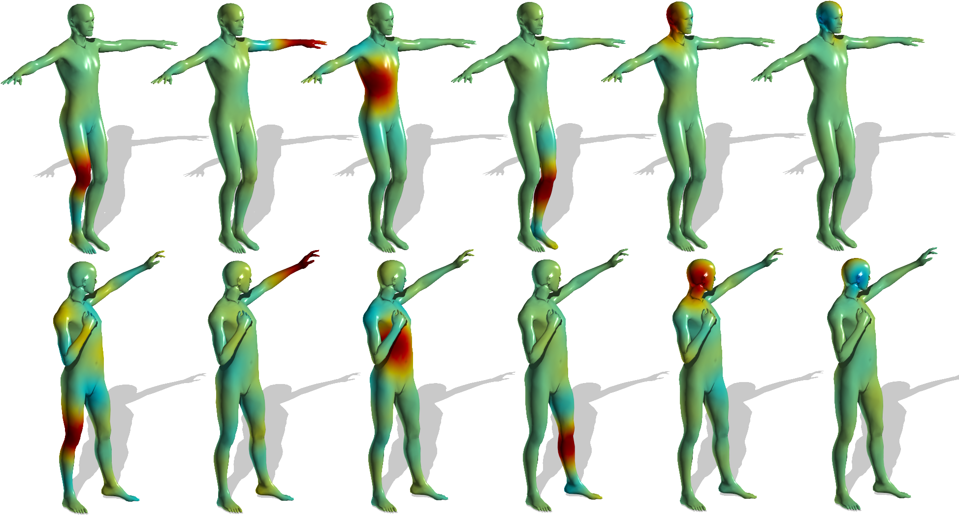
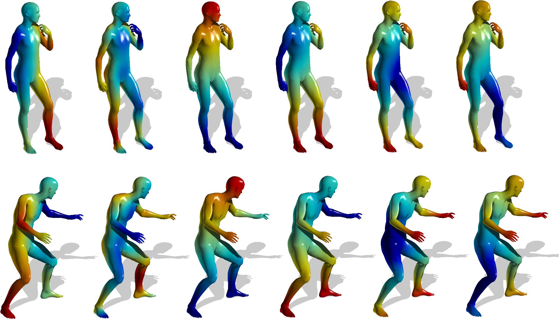
Figure 1: Mapping functions between two almost isometric shapes via S-GMDS.

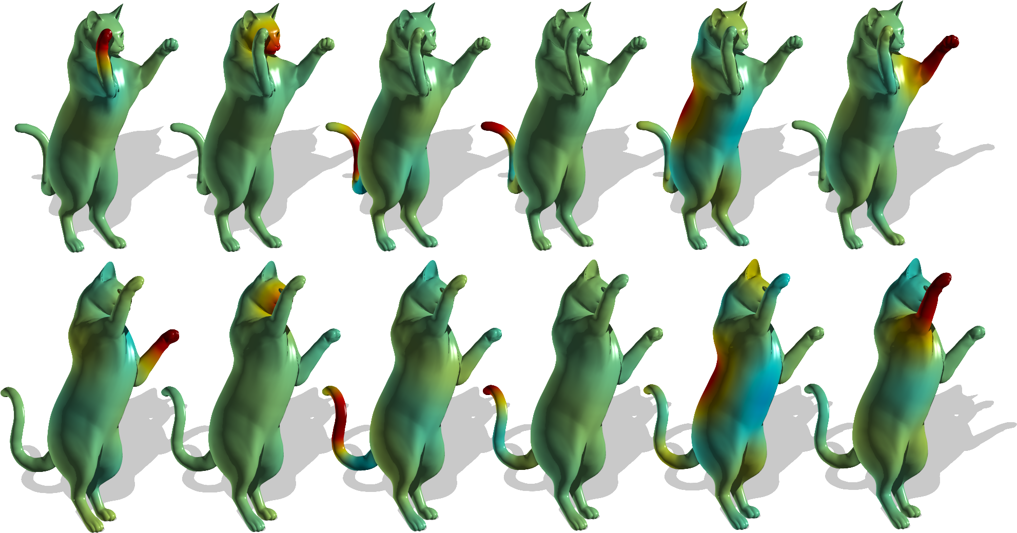
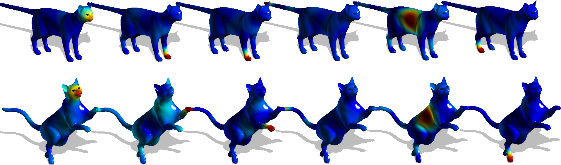
Figure 2: Mapping functions between two almost isometric shapes via S-GMDS.

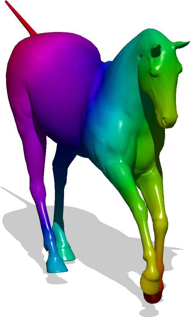
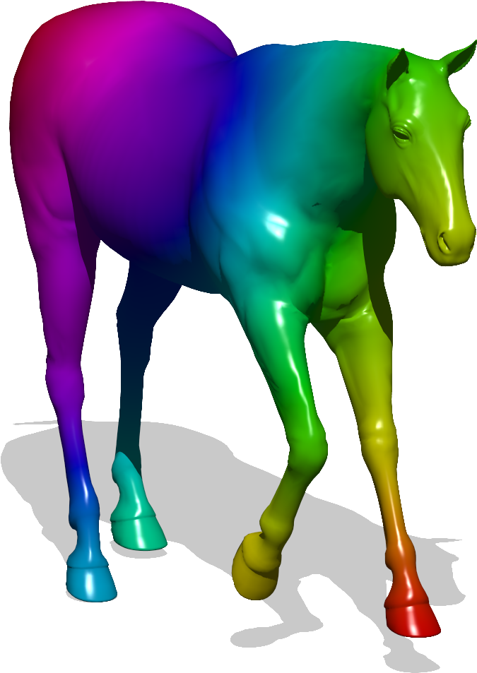
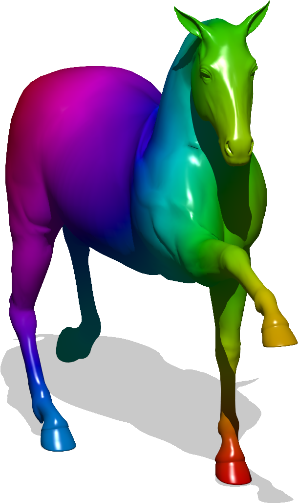
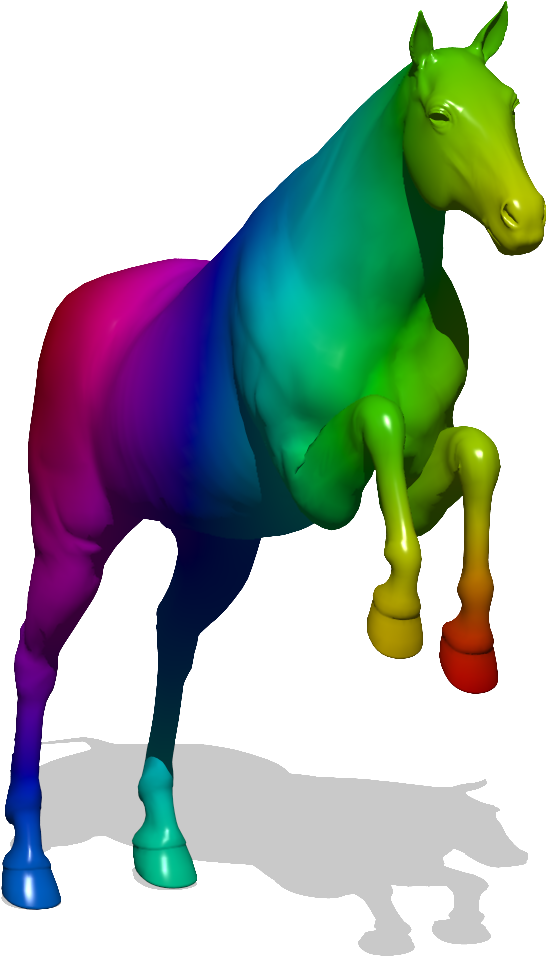
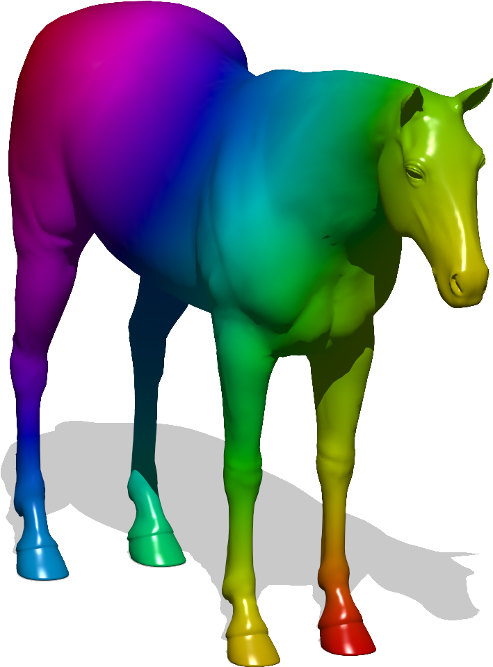
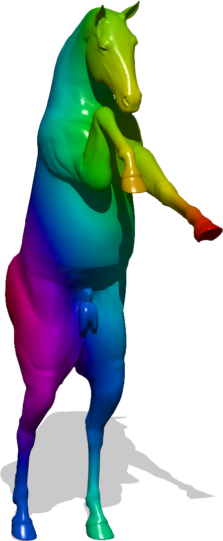
Figure 3: Dense point-to-point correspondence between six almost isometric shapes of a horse from the TOSCA dataset.

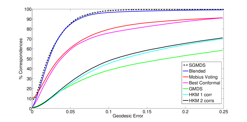
Figure 4: Quantitative evaluation of the S-GMDS applied to shapes from the TOSCA dataset, using the protocol from [27].

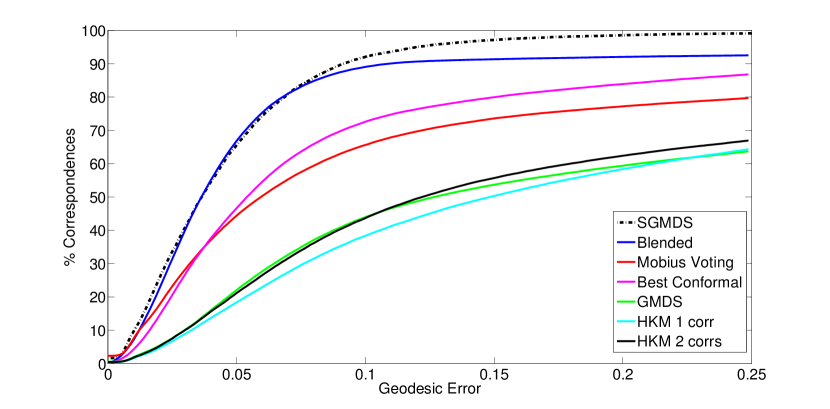
Figure 5: Quantitative evaluation of the S-GMDS on shapes from the SCAPE dataset, using the evaluation protocol from [27].

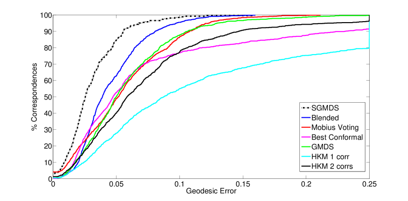
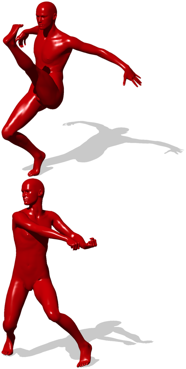
Figure 6: Performance evaluation of the S-GMDS compared to other methods applied to two “David” shapes from the TOSCA dataset which are relatively isometric. See shapes on the right. The comparison protocol is adopted from [27].

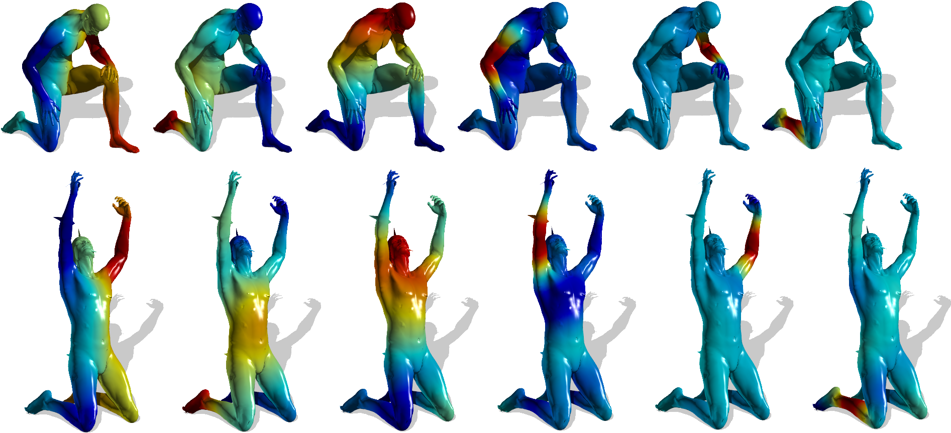
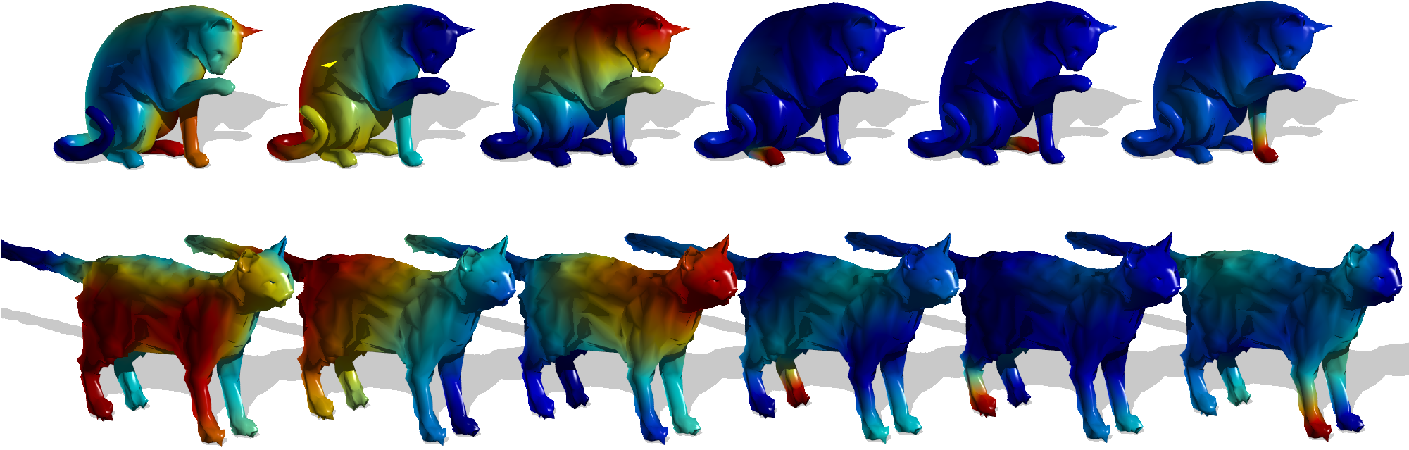
Figure 7: Mapping functions between two, almost isometric, noisy shapes via S-GMDS.

8 Conclusions

Spectral generalized multidimensional scaling method (S-GMDS) was proposed and proven to be an accurate model and efficient tool for matching non-rigid shapes. It accounts for almost isometric deformations of surfaces with respect to the regular metric. Being able to account for distortions of large as well as small distances when comparing two surfaces, with a natural regularization of the matching, reduces the need for support of heuristics or initializations. By incorporating the smoothness of the mapping, we treat the shape matching problem holistically rather than as an interpolation between multiple matched features such as points, regions, or localized functions.

Here, we used a regular metric in which geodesic distances on the surface determine the isometric quantity we try to preserve and whose distortions we use as a discrepancy measure. In our future research, we will try to axiomatically tackle the problem of analyzing objects between which local scale can be a substantial factor, yet, the conceptual meaning of such local structures with different scale is preserved. Though conformality could partially capture such distortions, we expect the scale invariant geometry introduced in [3] and plugged into the proposed framework to serve as the natural metric in such semi-local uniform scaling scenarios.

9 Acknowledgment

The authors would like to thank Alon Shtern for stimulating discussions and help with some of the computational tools. This work has been supported by grant agreement no. 267414 of the European Community s FP7-ERC program.

References

- [1] Yonathan Aflalo and Ron Kimmel. Regularized PCA. Submitted, 2013.
- [2] Yonathan Aflalo and Ron Kimmel. Spectral multi dimensional scaling. Proceedings of the National Academy of Sciences, 110(45), 2013.
- [3] Yonathan Aflalo, Ron Kimmel, and Dan Raviv. Scale invariant geometry for non-rigid shapes. SIAM Journal on Imaging Sciences, 2013.
- [4] Yonathan Aflalo, Ron Kimmel, and Michael Zibulevsky. Conformal mapping with as uniform as possible conformal factor. SIAM Journal on Imaging Sciences, 6(1):78–101, 2013.
- [5] Dragomir Anguelov, Praveen Srinivasan, Hoi-Cheung Pang, Daphne Koller, Sebastian Thrun, and James Davis. The correlated correspondence algorithm for unsupervised registration of nonrigid surfaces. Advances in neural information processing systems, 17:33–40, 2004.
- [6] Mathieu Aubry, Ulrich Schlickewei, and Daniel Cremers. The wave kernel signature: A quantum mechanical approach to shape analysis. In Computer Vision Workshops (ICCV Workshops), 2011 IEEE International Conference on, pages 1626–1633. IEEE, 2011.
- [7] Aharon Ben-Tal and Michael Zibulevsky. Penalty/barrier multiplier methods for convex programming problems. SIAM Journal on Optimization, 7(2):347–366, 1997.
- [8] P. Bérard, G. Besson, and S. Gallot. Embedding riemannian manifolds by their heat kernel. Geometric and Functional Analysis, 4(4):373–398, 1994.
- [9] Paul J Besl and Neil D McKay. Method for registration of 3-d shapes. In Robotics-DL tentative, pages 586–606. International Society for Optics and Photonics, 1992.
- [10] I. Borg and P. Groenen. Modern Multidimensional Scaling: Theory and Applications. Springer, 1997.
- [11] Alexander M Bronstein, Michael Bronstein, Michael M Bronstein, and Ron Kimmel. Numerical geometry of non-rigid shapes. Springer, 2008.
- [12] Alexander M Bronstein, Michael M Bronstein, and Ron Kimmel. Efficient computation of isometry-invariant distances between surfaces. SIAM Journal on Scientific Computing, 28(5):1812–1836, 2006.
- [13] Alexander M. Bronstein, Michael M. Bronstein, and Ron Kimmel. Generalized multidimensional scaling: A framework for isometry-invariant partial surface matching. Proceedings of the National Academy of Sciences of the United States of America, 103(5):1168–1172, 2006.
- [14] Alexander M Bronstein, Michael M Bronstein, Ron Kimmel, Mona Mahmoudi, and Guillermo Sapiro. A gromov-hausdorff framework with diffusion geometry for topologically-robust non-rigid shape matching. International Journal of Computer Vision, 89(2-3):266–286, 2010.
- [15] M. M. Bronstein, A. M. Bronstein, R. Kimmel, and I. Yavneh. Multigrid multidimensional scaling. Numerical Linear Algebra with Applications, 13(2-3):149–171, 2006.
- [16] Dmitri Burago, Yuri Burago, and Sergei Ivanov. A course in metric geometry, volume 33. American Mathematical Society Providence, 2001.
- [17] Yang Chen and Gérard Medioni. Object modeling by registration of multiple range images. In Robotics and Automation, 1991. Proceedings., 1991 IEEE International Conference on, pages 2724–2729. IEEE, 1991.
- [18] R. R. Coifman and S. Lafon. Diffusion maps. Applied and Computational Harmonic Analysis, 21(1):5 – 30, 2006. Special Issue: Diffusion Maps and Wavelets.
- [19] A. Dubrovina and R. Kimmel. Approximately isometric shape correspondence by matching pointwise spectral features and global geodesic structures. Advances in Adaptive Data Analysis, 3(1-2):203–228, 2011.
- [20] A. Elad and R. Kimmel. On bending invariant signatures for surfaces. IEEE Trans. Pattern Analysis and Machine Intelligence (PAMI), 25(10):1285–1295, 2003.
- [21] K Gȩbal, J Andreas Bærentzen, Henrik Aanæs, and Rasmus Larsen. Shape analysis using the auto diffusion function. In Computer Graphics Forum, volume 28, pages 1405–1413. Wiley Online Library, 2009.
- [22] Teofilo F Gonzalez. Clustering to minimize the maximum intercluster distance. Theoretical Computer Science, 38:293–306, 1985.
- [23] M. Gromov. Structures metriques pour les varietes riemanniennes. Textes Mathematiques, no. 1, 1981.
- [24] Xianfeng Gu, Yalin Wang, Tony F Chan, Paul M Thompson, and Shing-Tung Yau. Genus zero surface conformal mapping and its application to brain surface mapping. Medical Imaging, IEEE Transactions on, 23(8):949–958, 2004.
- [25] Dorit S Hochbaum and David B Shmoys. A best possible heuristic for the k-center problem. Mathematics of operations research, 10(2):180–184, 1985.
- [26] Miao Jin, Yalin Wang, S-T Yau, and Xianfeng Gu. Optimal global conformal surface parameterization. In Visualization, 2004. IEEE, pages 267–274. IEEE, 2004.
- [27] Vladimir G. Kim, Yaron Lipman, and Thomas Funkhouser. Blended intrinsic maps. In ACM SIGGRAPH 2011 papers, SIGGRAPH ’11, pages 79:1–79:12, New York, NY, USA, 2011. ACM.
- [28] R. Kimmel and J. A. Sethian. Computing geodesic paths on manifolds. In Proc. Natl. Acad. Sci. USA, pages 8431–8435, 1998.
- [29] A. Kovnatsky, M. M. Bronstein, A. M. Bronstein, K. Glashoff, and R. Kimmel. Coupled quasi-harmonic basis. Computer Graphics Forum (EUROGRAPHICS), 2013.
- [30] Bruno Lévy. Laplace-Beltrami eigenfunctions towards an algorithm that “understands” geometry. In Shape Modeling and Applications, 2006. SMI 2006. IEEE International Conference on, pages 13–13. IEEE, 2006.
- [31] Yaron Lipman and Ingrid Daubechies. Surface comparison with mass transportation. Advances in Mathematics, 227(3), June 2011.
- [32] Yaron Lipman and Thomas Funkhouser. Möbius voting for surface correspondence. ACM Transactions on Graphics (Proc. SIGGRAPH), 28(3), August 2009.
- [33] Diana Mateus, Radu Horaud, David Knossow, Fabio Cuzzolin, and Edmond Boyer. Articulated shape matching using laplacian eigenfunctions and unsupervised point registration. In Computer Vision and Pattern Recognition, 2008. CVPR 2008. IEEE Conference on, pages 1–8. IEEE, 2008.
- [34] Facundo Memoli. On the use of Gromov-Hausdorff distances for shape comparison. In M. Botsch, R. Pajarola, B. Chen, and M. Zwicker, editors, Symposium on Point Based Graphics, pages 81–90, Prague, Czech Republic, 2007. Eurographics Association.
- [35] Facundo Memoli and G. Sapiro. A theoretical and computational framework for isometry invariant recognition of point cloud data. Found. Comput. Math., 5(3):313–347, 2005.
- [36] Niloy J Mitra, Natasha Gelfand, Helmut Pottmann, and Leonidas Guibas. Registration of point cloud data from a geometric optimization perspective. In Proceedings of the 2004 Eurographics/ACM SIGGRAPH symposium on Geometry processing, pages 22–31. ACM, 2004.
- [37] M. Ovsjanikov, M. Ben-Chen, J. Solomon, A. Butscher, and L. Guibas. Functional maps: a flexible representation of maps between shapes. ACM Trans. Graph., 31(4):30:1–30:11, July 2012.
- [38] U. Pinkall and K Polthier. Computing discrete minimal surfaces and their conjugates. Experimental mathematics, 2(1):15–36, 1993.
- [39] Jonathan Pokrass, Alexander M. Bronstein, Michael M. Bronstein, Pablo Sprechmann, and Guillermo Sapiro. Sparse modeling of intrinsic correspondences. Computer Graphics Forum (EUROGRAPHICS), 32:459–268, 2013.
- [40] D. Raviv, A. M. Bronstein, M. M. Bronstein, and R. Kimmel. Full and partial symmetries of non-rigid shapes. International Journal of Computer Vision (IJCV), 89:18–39, August 2009.
- [41] Dan Raviv, Anastasia Dubrovina, and Ron Kimmel. Hierarchical matching of non-rigid shapes. In Scale Space and Variational Methods in Computer Vision, pages 604–615. Springer, 2012.
- [42] Guy Rosman, Alexander M Bronstein, Michael M Bronstein, Avram Sidi, and Ron Kimmel. Fast multidimensional scaling using vector extrapolation. SIAM J. Sci. Comput., 2, 2008.
- [43] R. Rustamov, M. Ovsjanikov, O. Azencot, M. Ben-Chen, F. Chazal, and L. Guibas. Map-based exploration of intrinsic shape differences and variability. In SIGGRAPH. ACM, 2013.
- [44] Y Sahillioğlu and Yucel Yemez. Coarse-to-fine combinatorial matching for dense isometric shape correspondence. In Computer Graphics Forum, volume 30, pages 1461–1470. Wiley Online Library, 2011.
- [45] E. L. Schwartz, A. Shaw, and E. Wolfson. A numerical solution to the generalized mapmaker’s problem: Flattening nonconvex polyhedral surfaces. IEEE Trans. Pattern Anal. Mach. Intell., 11(9):1005–1008, September 1989.
- [46] J. Sun, M. Ovsjanikov, and L. Guibas. A concise and provably informative multi-scale signature based on heat diffusion. In Proceedings of the Symposium on Geometry Processing, SGP ’09, pages 1383–1392, Aire-la-Ville, Switzerland, Switzerland, 2009. Eurographics Association.
- [47] Andrei Zaharescu, Edmond Boyer, Kiran Varanasi, and Radu Horaud. Surface feature detection and description with applications to mesh matching. In Computer Vision and Pattern Recognition, 2009. CVPR 2009. IEEE Conference on, pages 373–380. IEEE, 2009.
- [48] Wei Zeng, Lok Ming Lui, Feng Luo, Tony Fan-Cheong Chan, Shing-Tung Yau, and David Xianfeng Gu. Computing quasiconformal maps using an auxiliary metric and discrete curvature flow. Numerische Mathematik, 121(4):671–703, 2012.
- [49] Yun Zeng, Chaohui Wang, Yang Wang, Xianfeng Gu, Dimitris Samaras, and Nikos Paragios. Dense non-rigid surface registration using high-order graph matching. In Computer Vision and Pattern Recognition (CVPR), 2010 IEEE Conference on, pages 382–389. IEEE, 2010.
- [50] G. Zigelman, R. Kimmel, and N. Kiryati. Texture mapping using surface flattening via multidimensional scaling. Visualization and Computer Graphics, IEEE Transactions on, 8(2):198–207, 2002.