Prompt Optical Emission from Gamma-ray Bursts with Non-single Timescale Variability of Central Engine Activities

Abstract

The complete high-resolution lightcurves of Swift GRB 080319B present an opportunity for detailed temporal analysis of the prompt optical emission. With a two-component distribution of initial Lorentz factors, we simulate the dynamical process of the ejected shells from the central engine in the framework of the internal shock model. The emitted radiation are decomposed into different frequency ranges for a temporal correlation analysis between the lightcurves in different energy bands. The resulting prompt optical and gamma-ray emission show similar temporal profiles, both as a superposition of a slow variability component and a fast variability component, except that the gamma-ray lightcurve is much more variable than its optical counterpart. The variability features in the simulated lightcurves and the strong correlation with a time lag between the optical and gamma-ray emission are in good agreement with the observations of GRB 080319B. Our simulations suggest that the variations seen in the lightcurves stem from the temporal structure of the shells injected from the central engine of gamma-ray bursts. The future high temporal resolution observations of prompt optical emission from GRBs, e.g., by UFFO-Pathfinder and SVOM-GWAC, provide a useful tool to investigate the central engine activity.

1 Introduction

Gamma-ray bursts (GRBs) are believed to be produced by the relativistic jets released from the compact central engines, however the composition of jets and the energy dissipation and radiation mechanism at work are still far from clear. In the widely used internal shock model ([Rees & Mészáros 1994]), the energy dissipation in GRBs is caused by collisions between different parts of the unsteady outflow. These collisions produce shocks which accelerate electrons and generate magnetic field, and the GRB prompt emission is produced by the synchrotron radiation from the accelerated electrons. The internal shock model can generally match the gamma-ray properties of GRBs. For typical model parameters, the internal shock synchrotron model can naturally explain the complexity of GRB light curves ([Kobayashi et al. 1997]), the spectral break energy around MeV range, and the high energy photon index of $\beta\sim-2$ (see review of [Waxman 2003]). Moreover the ”fast cooling problem” of the low energy photon index can also be reconciled by involving postshock magnetic field decay in the internal shock model ([Pe’er & Zhang 2006, Zhao et al. 2013]).

The observations of GRB prompt emission outside the MeV energy range will further help to diagnose the jet properties and the central engine activity. The Fermi-LAT observations of bright GRBs reveal that the GRB emission in GeV range also shows short timescale, $\la 1$ s, variabilities in both long and short GRBs (e.g., [Abdo et al. 2009a, Abdo et al. 2009b]), implying the similar origin related to MeV emission. However, the temporal delay of GeV emission relative to MeV one implies larger radii of GeV emission than that of MeV ones ([Li 2010]). Moreover, the fact that the GeV emission is dominated by MeV one supports that the radiation mechanism at work for MeV emission is synchrotron radiation other than inverse-Compton scattering ([Wang et al. 2009]; see also [Derishev et al. 2001, Piran et al. 2009]). On the other hand, the prompt optical emission during the gamma-ray emission is detected in some GRBs (e.g., GRB 990123, [Akerlof et al. 1999]; GRB 041219A, [Vestrand et al. 2005]; GRB 051109A and GRB 051111, [Yost et al. 2007]; GRB 061121, [Page et al. 2007]; see also [Kopač et al. 2013], and references therein). The bright optical emission also implies that the radius of the optical emission region is larger than MeV one, in order to avoid the synchrotron self absorption (Li & Waxman [2008, Fan et al. 2009, Shen& Zhang 2009, Zou et al. 2009]). However the temporal optical properties in short time scale, $\la 1$ s, are not clear due to the low time resolution in optical observations.

By luck, the detection of the naked-eye burst, GRB 080319B, presents the only and best-sampled case hitherto for analyzing the overall temporal structure of the lightcurves of GRBs ([Racusin et al. 2008]; Beskin et al. [2010]). The high (sub-second) temporal resolution data, acquired from the onset of the optical transient to the end, makes the burst possible for revealing the detailed structure of the optical emission, shedding light on the behavior of the burst internal engine (Beskin et al. [2010]). There are two main temporal properties in the optical light curve of GRB 080319B. First, the onset of the optical emission is delayed relative to the gamma-ray one by $\sim 10$s; Second, in the plateau phase the optical light curve is correlated to gamma-ray one but with a time lag of $\sim 2$s. The former property may be due to the effect of environment, e.g., the dust effect in the molecular cloud ([Cui et al. 2013]), while the latter is more likely tracking the time history of the central engine, which is the focus of this paper.

As pointed out in Li & Waxman ([2008]), within the context of the internal shock models, after the first generation collisions producing gamma-ray emission, collisions continue to happen in larger and larger radii with smaller and smaller relative velocities. These ”residual collisions” produce longer and longer wavelength emission, which can avoid the strong synchrotron absorption in gamma-ray emission region and produce strong optical emission as observed. Because of the larger emission radii, the optical emission is expected to systemically delay relative to the gamma-ray one. Moreover the correlation between optical and gamma-ray light curves in GRB 080319B implies a large timescale modulation in the central engine activity.

In this paper we carry out numerical simulations of internal shocks to produce multi-band, including gamma-ray and optical, light curves, with focus on the effect of non-single timescale activities of the central engines. In Section 2, we provide a general description of the model we use. In Section 3, based on the model, we perform several simulation tests with different initial Lorentz factor distributions, following which we derive both optical and gamma-ray lightcurves with different temporal structures. In Section 4, we compare the model results with the observational data of GRB 080319B. We discuss the implications on the central engine activity in Section 5, and draw our conclusions in Section 6.

2 Model

The GRB unsteady outflow can be approximated by a set of individual shells with the initial position $r_{i}$, mass $m_{i}$, Lorentz factor $\gamma_{i}$ and width $\Delta_{i}$ ($i=1,...,N$) at time $t=0$. The initial widths can be taken to be the size of the source, $\Delta_{1,...,N}=\Delta_{0}\approx 10^{6}$cm. Given the initial condition of the shells, the dynamical evolution afterward will be totally fixed. Two neighboring shells $i$ and $i+1$ which satisfy $v_{i+1}>v_{i}$ may collide at a time of $t+\Delta t$, where $\Delta t=(r_{i}-r_{i+1})/(v_{i+1}-v_{i})$, and the colliding radius is $r_{c}=r_{i}+v_{i}\Delta t=r_{i+1}+v_{i+1}\Delta t$. The pair of shells with smaller $\Delta t$ will collide first and merge into a new shell.

For the pair of colliding shells, the velocity of center of momentum (c.m.) is $\beta_{cm}=\sum\gamma_{i}\beta_{i}m_{i}/\sum\gamma_{i}m_{i}=\sum m_{i}\sqrt{\gamma_{i}^{2}-1}/\sum\gamma_{i}m_{i}$ and the relevant Lorentz factor (LF) is $\gamma_{cm}=1/\sqrt{1-\beta_{cm}^{2}}$. They are also the velocity and LF of the merged shell, respectively. In the case of $\gamma_{i,i+1}\gg 1$, the c.m. LF can be approximated by

$$\gamma_{cm}=\sqrt{\frac{\gamma_{i}m_{i}+\gamma_{i+1}m_{i+1}}{m_{i}/\gamma_{i}+m_{i+1}/\gamma_{i+1}}}.$$ (1)

The shell may expand and change the shell width. Before collision at $r_{c}$, the width of a shell is $\Delta_{i}=\max(\Delta_{i},~{}r_{c}/\gamma_{cm}^{2})$ ([Guetta et al. 2001]). Because of compression by the shocks, the width of the merged shell right after shock crossing, $\Delta_{c}$, is smaller than the sum of the shell widths right before the collision $\Delta_{c}<\Delta_{i}+\Delta_{i+1}$ (We derive $\Delta_{c}$ in the appendix). After merging, the parameters for merged shell are the position $r_{c}$, mass $m_{i}+m_{i+1}$, LF $\gamma_{cm}$ and width $\Delta_{c}$. Collisions continue to occur, and they will only stop when the shell velocities are increasing with radius after enough collisions and momentum exchanges between shells.

The internal energy generated in this collision is

$$E_{in}/c^{2}=(\gamma_{i}m_{i}+\gamma_{i+1}m_{i+1})-\gamma_{cm}(m_{i}+m_{i+1})$$ (2)

which is released by synchrotron radiation. The emission appears as a pulse in the light curve. For simplicity we assume the shape of the pulse as a rectangle with a width of $\delta t=r_{c}/2\gamma_{cm}^{2}c$. So the luminosity of the light curve pulse is $L=E_{in}/\delta t$. Actually, a pulse with fast rise and slower decline in lightcurves can be produced due to the effect of equal arrival time surface (e.g., [Kobayashi et al. 1997, Shen et al. 2005, Huang et al. 2007]). However, the time resolution of the observed lightcurves in the prompt phase is not sufficient to tell the detailed pulse shapes. Thus we adopt a simple shape for each pulse and this assumption does not affect our temporal analysis of the lightcurves. In observation, the starting time of the pulse is at a observer time of

$$t_{\rm obs}=t-r_{c}/c.$$ (3)

For the numerous collisions taking place between multiple shells, we superimpose pulses produced by each collision according to their time sequence.

Let us calculate the characteristic energy of the synchrotron photons. The shell $i$’s velocity and LF in c.m. frame are

$$\beta^{\prime}=\frac{\beta_{i}-\beta_{cm}}{1-\beta_{i}\beta_{cm}},~{}~{}\gamma^{\prime}=\gamma_{i}\gamma_{cm}(1-\beta_{i}\beta_{cm}).$$ (4)

The characteristic postshock electron LF is

$$\gamma_{e}\approx(\gamma^{\prime}-1)\epsilon_{e}m_{p}/m_{e}+1,$$ (5)

where $\epsilon_{e}$ is the fraction of postshock energy carried by electrons. The magnetic field in the shock frame is given by

$$B=\sqrt{\frac{2\epsilon_{B}E_{in}}{\gamma_{cm}^{2}r_{c}^{2}\Delta_{c}}},$$ (6)

where $\epsilon_{B}$ is the fraction of postshock energy carried by magnetic field. Note here we use the shock-compressed width $\Delta_{c}$ (derived in the appendix) to calculate $B$. The synchrotron photon energy is then

$$\epsilon_{syn}\approx\gamma_{cm}\gamma_{e}^{2}\frac{heB}{2\pi m_{e}c}=\gamma_{e}^{2}\frac{he}{2\pi m_{e}c}\sqrt{\frac{2\epsilon_{B}E_{in}}{r_{c}^{2}\Delta_{c}}}$$ (7)

independent of $\gamma_{cm}$. The equipartition values $\epsilon_{e}=\epsilon_{B}=1/3$ will be used in the following numerical simulation.

For long wavelength emission, the synchrotron absorption may be important. Following Li & Waxman ([2008]) to calculate the synchrotron absorption frequency when $\epsilon_{a}>\epsilon_{syn}$, we have

$$\epsilon_{a}=2(\epsilon_{B}E_{in})^{1/14}\gamma_{cm}^{4/7}\gamma^{\prime 2/7}(m_{i}+m_{i+1})^{2/7}(cr_{c})^{-5/7}\Delta_{c}^{-5/14}\rm keV,$$ (8)

where a flat electron distribution of $p=2$ is used. The energy spectrum will peak at $\epsilon=\max(\epsilon_{syn},\epsilon_{a})$. For simplicity let us assume a $\delta$ function for the spectrum, i.e., the radiation is emitted at $\epsilon$.

In order to inspect the temporal correlation between the prompt optical and gamma-ray emission, the radiation produced by two shell collisions is decomposed into different frequency ranges, gamma-ray ($>100$ keV), X-ray ($1-10$ keV) and optical emission ($1-10$ eV), according to the energy band at which the synchrotron emission peaks.

3 Simulation tests

In order to show the effect of multi-timescale variabilities on the dynamics of the outflow, we carry out simulations for both cases of single- and two-timescale variabilities for comparison. We consider a series of individual material shells $i=1,2,...,N$, with total shell number $N$, released in a duration of $T=20$ s, so that the interval between two nearby shells is $\tau_{1}=T/N$. The shells have equal masses but different LFs. We carry four simulation tests as below. For Test 1, we use $N=2000$, thus $\tau_{1}=10$ ms, and the bulk LF of each shell follows

$$\log\gamma_{i}=\log 50+\xi_{i}\log 10+(2\xi_{i}-1)\log 2,$$ (9)

where $\xi_{i}$ is the random number between zero and unity. This is the case with only a single timescale of $\tau_{1}=10$ ms. For Test 2, there are two timescales in the LF evolution. Beside the $\tau_{1}=10$ ms variability ($N=2000$), there is an additional slow modulation of $\tau_{2}=5$ s,

$$\log\gamma_{i}=\log 50+\xi_{i}\log 10+\sin[\frac{2\pi}{\tau_{2}}(i-1)\tau_{1}-1.5]\log 2.$$ (10)

We also test Test 3 and 4 similar to Test 2 but with different values of $\tau_{1}$ or $\tau_{2}$: $\tau_{1}=10$ ms and $\tau_{2}=3.3$ s in Test 3; while $\tau_{1}=40$ ms (i.e., $N=500$) and $\tau_{2}=5$ s in Test 4.

Test 1.

To examine the dependence of the temporal structure of lightcurves on the initial velocity variations inside the ejecta, we first perform a simulation test using a succession of initial Lorentz factors with only a rapid random variability component. We consider the case with uniformly distributed LFs presented in Fig. 2. Note that here we only display the first 20 s of the optical lightcurve for a clear comparison with the gamma-ray one. It is straightforward to show that the short-scale variability features of the LFs are imprinted on both the optical and gamma-ray lightcurves (Fig. 2). In contrast to the broad periodic component seen in the following simulation tests, there are only stochastic spikes existing in the lightcurves.

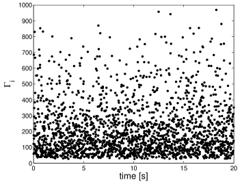
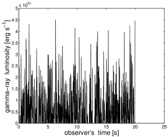
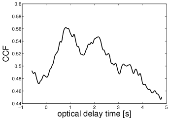
Figure 1: Results of Test 1. Top panel: the initial Lorentz factor distribution. Second panel: the optical light curve Third panel: the gamma-ray lightcurve in 50 ms time bin. Bottom panel: the cross-correlation function between the gamma-ray and optical lightcurves.

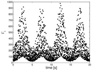
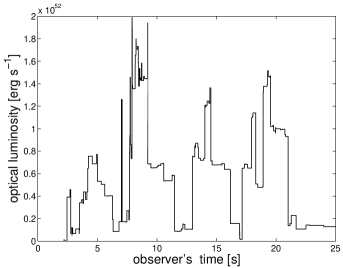
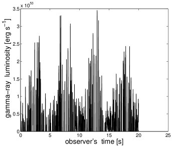
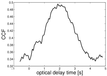
Figure 2: Results of Test 2.

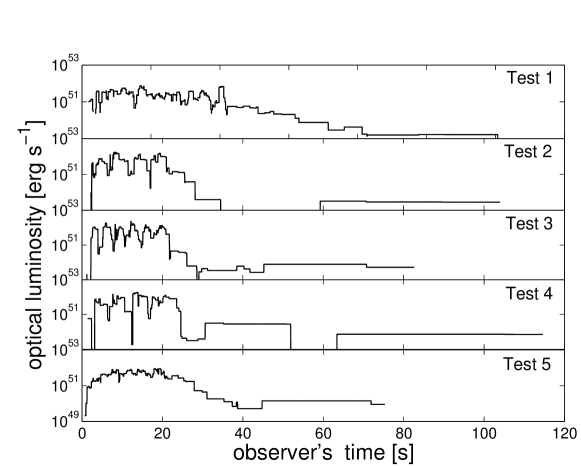
Figure 6: The complete optical lightcurves from all simulation tests.

In addition, Fig. 6 shows the complete optical lightcurves from our five simulation tests. Logarithmic luminosity is used here due to the weak optical emission after $t_{\rm obs}>20$ s. The optical emission clearly has a more variable temporal profile in the early 20 s than the rest part (also see Table 1), i.e., the variability time in the late time is larger than the early, $<20$s, emission.

Test 2.

We start with a simple two-component Lorentz factor distribution of the shells. Fig. 2 presents the distribution of the initial LFs of the shells with indices from one to $N$. In our calculations, the $N$th shell is the first shell emitted by the inner engine, indicating the outer edge of the ejecta. The overall duration of the burst is $T=20$ s in the observer frame. The slow and periodic variability existing in the LFs is on a time scale of $\tau_{2}=5$ s, and the overlapping rapid and irregular variations have $\tau_{1}=10$ ms time scale. Fig. 2 shows the corresponding optical and gamma-ray lightcurves produced by a Monte-Carlo simulation of the dynamic process of the colliding shells we described in Section 2.

By comparing these two lightcurves, we find they both show a superposition of two variability components: a slow periodic component with a duration of $\sim$ 5 s and a fast component with stochastic short pulse widths. But in contrast to the smoother profile in optical band, the gamma-ray lightcurve is obviously highly variable with more rapid short-scale variabilities (see Table 1). To have a better comparison with the observed data, we rebinned the optical and gamma-ray lightcurves with a 0.13 s and 50 ms bin size, respectively (Beskin et al. [2010]), and performed a cross-correlation analysis between them. Fig. 2 displays the normalized cross-correlation sequence between the optical and gamma-ray lightcurves as a function of optical delay time.The correlation coefficient reaches its highest value ($\sim$ 0.50) when the optical flux is delayed by 1.9 s with respect to the gamma-ray emission. Since our results are just based on the simple modeling of the internal shock dynamics, the time delay naturally results from the evolution of Lorentz factor fluctuations of the fast moving shells. At first, gamma-ray emission originates from the outflow with highly variable LFs at a small radius. As the flow moves forward to a larger radius, the variance of the Lorentz factors of the remained shells decreases, leading to the decrease of the radiated energy after collisions, and the characteristic frequency of the emission as well (Li & Waxman [2008]).

The average ratio of the optical and gamma-ray fluxes indicates relatively bright optical emission accompanying gamma-ray emission, which is consistent with optical detections. The bright optical emission can be naturally explained in the framework of the residual collisions model, since optical emission can be produced at large radii, where the optical depth to optical photons is low (Li & Waxman [2008]).

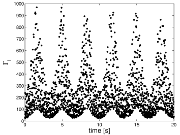
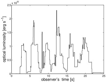
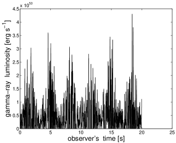
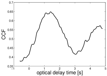
Figure 3: Results of Test 3.

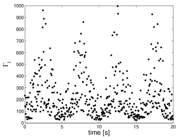
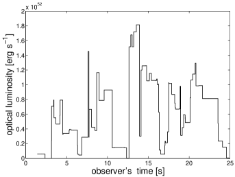
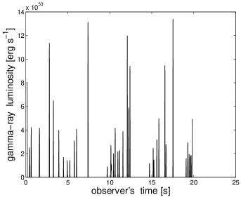
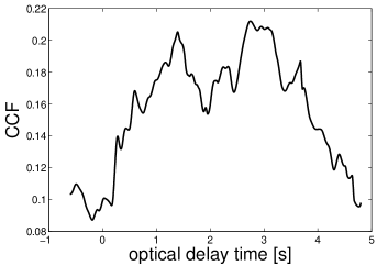
Figure 4: Results of Test 4.

Test 3.

Next, we test the cases with different timescales of the two variability components of the initial LFs respectively. This is the same as Test 2, except the period of the slow variability component is changed to 3.3 s. Fig. 4 shows the consequential optical and gamma-ray lightcurves. Similar results to those presented in Fig. 2 can be found for both lightcurves. With narrower slow component duration ($\sim$ 3.3 s), the lightcurves contain the same number of periodic variability seen in the initial LFs.

Test 4.

We then increase the timescale of the rapid variability of the initial LFs by reducing the number of shells. Correspondingly, the irregular short-scale variabilities in both lightcurves clearly have larger timescales. We find the total energy emitted over the gamma-ray band obviously decreases due to fewer collisions at small radii (see Fig. 4). Fewer gamma-ray data also lead to lower correlation between the two lightcurves.

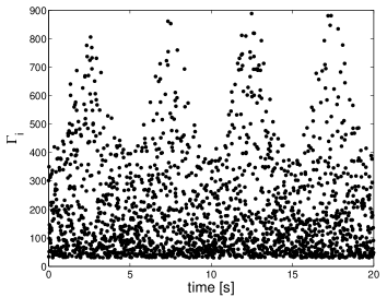
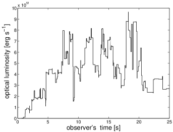
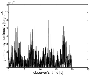
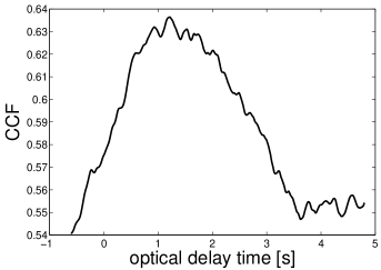
Figure 5: Results of Test 5, as a comparison with GRB 080319B (figure 2 in Beskin et al. ([2010])).

Table 1 lists the parameters for the above simulation tests. Here we do not consider the redshift of the source, or all the timescales in Table 1 should be increased by $1+\emph{z}$. As can be seen from our simulation tests, the temporal behavior of prompt optical and gamma-ray emission is sensitive to the changes of the initial velocity variations inside the ejecta. The variability features exhibited in lightcurves tend to strictly track the temporal structure of the initial LFs of the shells.

Table 1: Parameters and results of the simulation tests.

	$N$1	$\tau_{1}$ (s)2	$\tau_{2}$ (s)3	$r$4	$\Delta t$ (s)5	$\delta t_{o}$ (s)6	$\delta t_{o,1}$ (s)7	$\delta t_{o,2}$ (s)8	$\delta t_{\gamma}$ (s)9
Test 1	2000	0.01	$-$	0.56	0.8	2.8	1.4	12.9	0.004
Test 2	2000	0.01	5	0.50	1.9	3.0	1.3	15.0	0.004
Test 3	2000	0.01	3.3	0.65	1.4	2.3	1.4	13.5	0.006
Test 4	500	0.04	5	0.21	2.7	6.0	1.9	22.0	0.012
Test 5	2000	0.01	5	0.64	1.2	2.8	1.7	11.7	0.005

• The number of shells.

• The timescales of the fast variability components existing in initial LFs.

• The timescales of the slow variability components existing in initial LFs.

• The highest correlation coefficient between optical and gamma-ray lightcurves.

• The time lag between optical and gamma-ray emission.

• The average timescale of variability in optical emission.

• The average timescale of variability in optical emission for $t_{\rm obs}\leq 20$ s.

• The average timescale of variability in optical emission for $t_{\rm obs}>20$ s.

• The average timescale of variability in gamma-ray emission.

4 Comparison with GRB 080319B

The high temporal resolution detection of the prompt optical emission of GRB 080319B and its gamma-ray counterpart serve as the only available observed data to test our model. Periodic variability on a few seconds time scale may exist in both optical and rebinned gamma-ray lightcurves during the prompt phase of the emission (Beskin et al. [2010]). Besides the four similar peaks, short time-scale variability can be seen in the realistic lightcurves, including the rapid optical variability on time scales from several seconds to subseconds and a large amount of stochastic variability in the gamma-ray emission (Beskin et al. [2010]).

In align with the observations, the simulated lightcurves capture both the underlying equidistant broad component and the short-scale variability features. The detected time delay ($\sim$ 2 s in the observer frame, Beskin et al. [2010]) between the optical and gamma-ray emission has the same order of magnitude as $\Delta$ t shown in Table 1 (after multiplied by $1+\emph{z}$). Despite the time lag, a clear similarity exists between the optical and gamma-ray lightcurves, as indicated in Beskin et al. ([2010]). This temporal correlation shows the emission in the optical and gamma-ray ranges is generated by a common mechanism, but at different locations.

Since our model can be applied to general GRB events by modifying the initial Lorentz factor distribution of the ejected shells, in order to construct the temporal structure of this specific burst, we also present a slightly modified version of Test 2 (see Test 5 in Table 1 and Fig. 5) as a comparison with figure 2 in Beskin et al. ([2010]). Note that the initial LFs in Test 5 have the same variability timescales as those in Test 2, but the adjusted Lorentz factor distribution leads to different lightcurves characterized mainly by four overlapping peaks (Fig. 5) instead of separated pulses (Fig. 2).

5 Discussion

The simple model we proposed is able to explain the basic temporal structure of diverse GRB prompt emission. By adjusting the initial velocity variations, i.e., the initial Lorentz factor distribution in the outflow, our simulations can reproduce the complex variability features in realistic lightcurves. One can predict the highly variable temporal profile by controlling the initial variance of the shell velocities, and more importantly, inspecting the observational temporal features in the lightcurves of separate energy bands allows us to assess the central engine activity in detail.

The central engine activity and its detailed properties regulate the temporal variations displayed in the sequence of shells injected from the central engine, which are then reflected in the observed variability components in the lightcurves. For GRB 080319B, we require at least two timescales of the central engine activity to reproduce the observed optical light curve, which is an important implication of its central engine. In current situation we are not able to identify what causes these two timescales. However, following the common picture of the collapsar model a new black hole, with a surrounding torus, is born in the center of the progenitor star. For a black hole of $\sim 3m_{3}M_{\odot}$, the accretion time of material at the innermost radius $r_{\rm in}$ of the torus is $t_{\rm acc}\sim 2m_{3}$ ms (e.g., [Narayan et al. 2001]), comparable to the small timescale we require, whereas the accretion time at the outer radius $r_{\rm out}\sim 10^{2}r_{\rm in}$ is $t_{\rm acc}\sim 4m_{3}(r_{\rm out}/10^{2}r_{\rm in})^{3/2}$s ([Narayan et al. 2001]), similar to the larger timescale. This may imply that the material supply at the outer edge of the torus is non-stable.

An important feature shown in our simulation results is the time delay between the optical and gamma-ray lightcurves due to the larger radius of the optical emission region. The delay time is about 1 s in all the tests. The optical delay has been predicted by Li & Waxman ([2008]) in the single timescale case. They show that for optical emission to avoid the synchrotron self absorption, the outflow needs to expand to larger radii of $R\sim 10^{15}R_{15}$cm, and hence the optical delay time is $\Delta t\sim R/2\langle\Gamma\rangle^{2}c\sim 1R_{15}(\langle\Gamma\rangle/10^{2})^{-2}$s, where $\langle\Gamma\rangle$ is the average value of initial Lorentz factors of the ejected shells. This is comparable to the resulted delay time in the tests. However, since many factors can influence the delay time, more systematic simulations are required to investigate the dependence of the delay time on the input parameters in the future work.

6 Conclusions

Starting with a two-component Lorentz factor distribution of the shells injected from the central engine, our simulations generated the optical and gamma-ray lightcurves both as a superposition of two variability components with different time scales. The slow component has the same time scale as that exhibited in the initial LFs, while the time scale of the fast component has a trend with energy: the gamma-ray lightcurve has much more and faster short-scale variabilities than its optical counterpart. Moreover, the time scale of the fast variability changes with time in the simulated optical lightcurve. The value in the first 20 s of the lightcurve is one order of magnitude smaller than that of the rest part, which is in agreement with the finding in [Margutti et al. (2008)].

The similarity between the optical and gamma-ray lightcurves, and the time delay between them, provide strong evidence that the emission has a common origin, but is generated at different radii from the central engine. Further discussions show that the lightcurves of prompt emission actually provide the temporal information to clarify the physical nature of the central engine. The different variability components seen in the lightcurves depend on the intrinsic variability with different time scales of the internal engine. Detailed temporal analysis of the simulated lightcurves is necessary and will be performed in our future work.

Hopefully, more high temporal resolution observations of both prompt optical emission from GRBs will be acquired by future telescopes, e.g., UFFO-Pathfinder ([Chen et al. 2011]) and SVOM-GWAC ([Paul et al. 2011]). These well-sampled bursts will further test the validity of our model and provide a deeper insight into the source behavior.

appendix

We derive the width of the merged shell after shock crossings. Consider two colliding shells, with the lab-frame width $\Delta_{i}$ and LF $\gamma_{i}$, where $i=1,2$. Shell 2 is faster, and overtakes shell 1. There are double shocks and 4 regions in the interaction. The unshocked shell 1 and 2 have number densities $n_{1}$ and $n_{2}$, respectively, in their own rest frame. The densities in forward and reverse shock regions are $n_{f}=4\gamma_{f}n_{1}$ and $n_{r}=4\gamma_{r}n_{2}$, respectively, in their own rest frame, where $\gamma_{f,r}$ are the LFs of the shocked fluid relative to unshocked shell 1 and 2, respectively,

$$\gamma_{f}=\gamma_{1}\gamma_{cm}(1-\beta_{1}\beta_{cm}),~{}~{}\gamma_{r}=\gamma_{2}\gamma_{cm}(1-\beta_{2}\beta_{cm}).$$ (11)

Note there is no relative motion between forward and reverse shock regions.

Now consider everything in one frame, which is better to be the lab frame. In the lab frame, the unshocked shell 1, shocked fluid (both forward and reverse shock regions) and unshocked shell 2 have LFs $\gamma_{1}$, $\gamma_{cm}$ and $\gamma_{2}$. So in the lab frame, the densities of the 4 regions are, inner going, $\gamma_{1}n_{1}$, $\gamma_{cm}n_{f}$, $\gamma_{cm}n_{r}$ and $\gamma_{2}n_{2}$. The compression factor, i.e. the factor the density is enhanced by shock, is $k_{f}=\gamma_{cm}n_{f}/(\gamma_{1}n_{1})=4\gamma_{f}\gamma_{cm}/\gamma_{1}$ for forward shock region, or $k_{r}=\gamma_{cm}n_{r}/(\gamma_{1}n_{1})=4\gamma_{r}\gamma_{cm}/\gamma_{2}$ for reverse shock region. Thus the shock-compressed, merged shell has a width, right after merging without spreading, of

$$\Delta_{c}=\frac{\Delta_{1}}{k_{f}}+\frac{\Delta_{2}}{k_{r}}=\frac{\Delta_{1}\gamma_{1}}{4\gamma_{f}\gamma_{cm}}+\frac{\Delta_{2}\gamma_{2}}{4\gamma_{r}\gamma_{cm}}=\frac{1}{4\gamma_{cm}^{2}}\left(\frac{\Delta_{1}}{1-\beta_{1}\beta_{cm}}+\frac{\Delta_{2}}{1-\beta_{2}\beta_{cm}}\right).$$ (12)

References

- [Abdo et al. 2009a] Abdo, A. A., et al. 2009a, ApJ, 706, L138
- [Abdo et al. 2009b] Abdo, A. A., et al. 2009b, Nature, 462, 331
- [Akerlof et al. 1999] Akerlof, C., Balsano, R., Barthelmy, S., et al., 1999, Nature, 398, 400
- [Beloborodov 2010] Beloborodov A. M., 2010, MNRAS, 407, 1033
- [2010] Beskin, G., Karpov, S., Bondar, S., et al., 2010, ApJ, 719, L10
- [Chen et al. 2011] Chen, P. et al., 2011, eprint arXiv:1106.3929
- [Cui et al. 2013] Cui, X.-H., Li, Z., & Xin, L.-P. 2013, Research in Astronomy and Astrophysics, 13, 57
- [Derishev et al. 2001] Derishev, E. V., Kocharovsky, V. V., & Kocharovsky, V. V. 2001, A&A, 372, 1071
- [Fan et al. 2009] Fan, Y.-Z., Zhang, B., & Wei, D.-M. 2009, Phys. Rev. D, 79, 021301
- [Guetta et al. 2001] Guetta, D., Spada, M., & Waxman, E. 2001, ApJ, 557, 399
- [Huang et al. 2007] Huang, Y.-F., Lu, Y., Wong, A. Y. L., & Cheng, K. S., 2007, Chinese Journal of Astronomy and Astrophysics, 7, 397
- [Kobayashi et al. 1997] Kobayashi, S., Piran, T., & Sari, R., 1997, ApJ, 490, 92
- [Kopač et al. 2013] Kopač, D., Kobayashi, S., Gomboc, A., et al., 2013, ApJ, 772, 73
- [Lyutikov & Blandford 2003] Lyutikov, M., & Blandford, R., 2003, arXiv:astro-ph/0312347
- [Li 2010] Li, Z., 2010, ApJ, 709, 525
- [2008] Li, Z., & Waxman, E., 2008, ApJ, 674, 65
- [Lazzati et al. 2009] Lazzati, D., Morsony, B. J., & Begelman, M. C., 2009, ApJ, 700, L47
- [Mészáros & Rees 2000] Mészáros, P., & Rees, M. J., 2000, ApJ, 530, 292
- [Margutti et al. (2008)] Margutti, R., Guidorzi, C., Chincarini, G., et al., 2008, AIPC, 1065, 259
- [Narayan & Kumar 2009] Narayan, R., & Kumar, P., 2009, MNRAS, 394, L117
- [Narayan et al. 1992] Narayan, R., Paczyski, B., & Piran, T., 1992, ApJ, 395, L83
- [Narayan et al. 2001] Narayan, R., Piran, T., & Kumar, P. 2001, ApJ, 557, 949
- [Paul et al. 2011] Paul, J., Wei, J., Basa, S. & Zhang, S. 2011, CRPhy, 12, 298
- [Pe’er & Zhang 2006] Pe’er, A., & Zhang, B., 2006, ApJ, 653, 454
- [Piran et al. 2009] Piran, T., Sari, R., & Zou, Y.-C., 2009, MNRAS, 393, 1107
- [Page et al. 2007] Page, K. L., Willingale, R., Osborne, J. P., et al., 2007, ApJ, 663, 1125
- [Rees & Mészáros 1994] Rees, M. J., & Mészáros, P., 1994, ApJ, 430, L93
- [Racusin et al. 2008] Racusin, J. L., Karpov, S. V., Sokolowski, M., et al., 2008, Nature, 455, 183
- [Shen et al. 2005] Shen, R.-F., Song, L.-M., & Li, Z. 2005, MNRAS, 362, 59
- [Shen& Zhang 2009] Shen, R.-F., & Zhang, B., 2009, MNRAS, 398, 1936
- [Thompson 1994] Thompson, C., 1994, MNRAS, 270, 480
- [Usov 1994] Usov, V. V., 1994, MNRAS, 267, 1035
- [Vestrand et al. 2005] Vestrand, W. T., Wozniak, P. R., Wren, J. A., et al., 2005, Nature, 435, 178
- [Waxman 2003] Waxman, E., 2003, Supernovae and Gamma-Ray Bursters, 598, 393
- [Wang et al. 2009] Wang, X.-Y., Li, Z., Dai, Z.-G., & Mészáros, P., 2009, ApJ, 698, L98
- [Yost et al. 2007] Yost, S. A., Swan, H. F., Rykoff, E. S., et al., 2007, ApJ, 657, 925
- [Zhang & Yan 2011] Zhang, B., & Yan, H., 2011, ApJ, 726, 90
- [Zhao et al. 2013] Zhao, X., Li, Z., Liu, X., Zhang, B., Bai, J., & Meszaros, P., 2013, ApJ, submitted.
- [Zou et al. 2009] Zou, Y.-C., Piran, T., & Sari, R., 2009, ApJ, 692, L92