Pressure exerted by a vesicle on a surface

Abstract

Several recent works have considered the pressure exerted on a wall by a model polymer. We extend this consideration to vesicles attached to a wall, and hence include osmotic pressure. We do this by considering a two-dimensional directed model, namely that of area-weighted Dyck paths.

Not surprisingly, the pressure exerted by the vesicle on the wall depends on the osmotic pressure inside, especially its sign. Here, we discuss the scaling of this pressure in the different regimes, paying particular attention to the crossover between positive and negative osmotic pressure. In our directed model, there exists an underlying Airy function scaling form, from which we extract the dependence of the bulk pressure on small osmotic pressures.

1 Introduction

A polymer attached to a wall produces a force because of the loss of entropy on the wall. This has been measured experimentally [1, 2, 3] and recently described theoretically in two dimensions using lattice walk models [4, 5]. There has also been work concerning the entropic pressure of a polymer in the bulk [6]. Lattice walks and polygons on two dimensional lattices have in the past been utilised to model simple vesicles [7, 8, 9, 10, 11], where there can be an internal pressure. Here we explore the competition between the bulk internal pressure and the point pressure caused by entropy loss when a vesicle is fixed to a wall in two dimensions. Our study involves an exactly solved model of vesicles [10, 12], namely, area-weighted Dyck paths [13, 14, 15].

Let $Z_{N}$ be the partition function of some lattice model of rooted configurations of size $N$, for example directed or undirected self-avoiding walks or self-avoiding polygons, and let $Z_{N}^{(Q)}$ be the partition function conditioned on configurations avoiding a chosen point $Q$ in the lattice. Then the pressure on the point $Q$ is given by the difference of the finite-size free energies $-\log Z_{N}$ and $-\log Z_{N}^{(Q)}$, that is

$$P_{N}^{(Q)}=-\log Z_{N}^{(Q)}+\log Z_{N}\;.$$ (1.1)

Here we take $k_{B}T=1$ for convenience. When the configurations are Dyck paths, which are directed paths above the diagonal of a square lattice starting at the origin and ending on the diagonal, this model was analysed in [5]. The pressure at the point $Q=(m,m)$ for walks of length $2N$ is given exactly as

$$P_{N}^{(m)}=-\log\left(1-\frac{C_{m}C_{N-m}}{C_{N}}\right)\;,$$ (1.2)

where $C_{k}=\frac{1}{k+1}\binom{2k}{k}$ is the $k$-th Catalan number counting $2k$-step Dyck paths. For $N$ and $m$ large, this leads to

$$P_{N}^{(m)}=\frac{1}{\sqrt{\pi x^{3}(1-x)^{3}}}\cdot\frac{1}{N^{3/2}}+O(N^{-5/2})\;,$$ (1.3)

where $x=m/N$ measures the relative distance of the point $Q$ from the origin with respect to the length of the walk. That is, the pressure of the Dyck path decays to zero as $N^{-3/2}$ in the centre of the Dyck path, with an $x$-dependent profile, as shown in Figure 1.

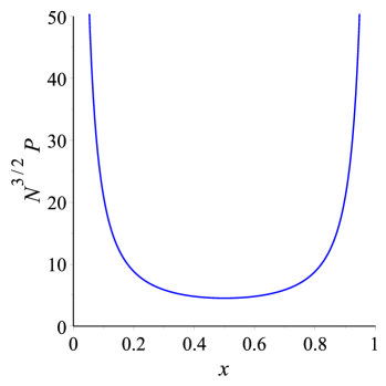
Figure 1: Pressure profile for long Dyck paths as a function of the relative distance $x$ from the point of tether.

In contrast, near the boundary the pressure tends to an $N$-independent limiting value

$$P_{N}^{(m)}\rightarrow-\log\left(1-\frac{C_{m}}{4^{m}}\right)\;.$$ (1.4)

2 The model

In an extension of the work described in the introduction, the configurations of the model studied here are area-weighted Dyck paths, where we have rotated the lattice by $45^{\circ}$ for convenience as shown in Figure 2. To be more precise, we weight each full square plaquette between the Dyck path and the surface with a weight $q=\exp(\Pi)$, where $\Pi$ is the osmotic pressure.

We use these paths to model vesicles adsorbed at the surface, that is to say that we consider them as vesicles with the bottom part of the membrane firmly attached to the surface. As described above, to calculate the pressure we need to consider a slightly modified set of configurations that avoid some point. For our vesicle model this means that the bottom of the vesicle does not include a particular plaquette, see Figure 2.

Figure 2: A vesicle of length 9 given by a Dyck path with 18 steps, enclosing the 11 shaded plaquettes and having weight $q^{11}$. When considering the modified configurations that avoid the lighter coloured plaquette, which is at distance $m=6$, the vesicle is considered to enclose 10 plaquettes and have weight $q^{10}$.

Denoting the set of all $2N$-step Dyck paths by ${\cal D}_{N}$, the partition function for unrestricted vesicles of length $N$ is given by

$$Z_{N}(q)=\sum_{\varphi\in{\cal D}_{N}}q^{A(\varphi)}\;,$$ (2.1)

where $A(\varphi)$ is the number of plaquettes enclosed by the configuration $\varphi$.

Similarly, denoting the set of all $2N$-step Dyck paths enclosing the surface plaquette at distance $1\leq m\leq N-1$ by ${\cal D}_{N}^{(m)}\subset{\cal D}_{N}$, the partition function for the restricted vesicles is given by

$$Z_{N}^{(m)}(q)=\sum_{\varphi\in{\cal D}_{N}^{(m)}}q^{A(\varphi)-1}\;.$$ (2.2)

Note that the distance $m$ is measured as the number of half-plaquettes along the surface to the point of interest.

The configurations in ${\cal D}_{N}\setminus{\cal D}_{N}^{(m)}$ are precisely the ones that touch the surface at distance $m$, whence

$$Z_{N}(q)-qZ_{N}^{(m)}(q)=\sum_{\varphi\in{\cal D}_{N}\setminus{\cal D}_{N}^{(m)}}q^{A(\varphi)}=Z_{m}(q)Z_{N-m}(q)\;.$$ (2.3)

For $q=1$ this reduces to Equation (1.2). Computing the pressure using Eqn. (1.1), we find that the pressure $P_{N}^{(m)}(q)$ of a Dyck vesicle of length $N$ on the surface at distance $m$ is given by

$$P_{N}^{(m)}(q)=-\log\left(1-\frac{Z_{m}(q)Z_{N-m}(q)}{Z_{N}(q)}\right)+\log q\;.$$ (2.4)

3 Results

3.1 Exact results

One can recursively calculate $Z_{N}(q)$ using

$$Z_{0}(q)=1\;,\quad Z_{N+1}(q)=\sum\limits_{k=0}^{N}q^{k}Z_{k}(q)Z_{N-k}(q)\;,\quad N\geq 0\;,$$ (3.1)

which for $q=1$ reduces to a well-known recursion for Catalan numbers. One sees that $Z_{N}(q)$, and therefore also $P_{N}^{(m)}(q)$, is computable in polynomial time. There are no closed-form expressions known.

However, there are well-known closed-form expressions [16, Example V.9] for the generating function

$$G(z,q)=\sum_{N=0}^{\infty}Z_{N}(q)z^{N}\;,$$ (3.2)

namely,

$$G(z,q)=\frac{A_{q}(z)}{A_{q}(z/q)},$$ (3.3)

where

$$A_{q}(z)=\sum_{n=0}^{\infty}\frac{q^{n^{2}}(-z)^{n}}{(q;q)_{n}}$$ (3.4)

is Ramanujan’s Airy function. Here, we use the $q$-product notation $(t;q)_{n}=\prod_{k=0}^{n-1}(1-tq^{k})$.

Note that the radius of convergence $z_{c}(q)$ of $G(z,q)$ is simply related to the thermodynamic limit of the partition function via

$$\log z_{c}(q)=-\lim_{N\to\infty}\frac{1}{N}\log Z_{N}(q)\;.$$ (3.5)

For $q=1$, $G(z,q)$ is simply the Catalan generating function and hence $z_{c}(1)=1/4$.

At the level of the generating function, the recurrence (3.1) is equivalent to the functional equation

$$G(z,q)=1+zG(z,q)G(qz,q)\;,$$ (3.6)

which in turn leads to a nice continued fraction representation for $G(z,q)$:

$$G(z,q)=\cfrac{1}{1-\cfrac{z}{1-\cfrac{qz}{1-\cfrac{q^{2}z}{1-\cfrac{q^{3}z}{1-\ldots}}}}}\;.$$ (3.7)

We can calculate the surface pressure in the thermodynamic limit from the generating function by relating the pressure to the density of contacts with the surface. In order to do so, we need to introduce a surface weight $\kappa$ for contacts with the surface, which we will set to one after the calculation. Let $G(z,q;\kappa)$ be the generating function for area-weighted Dyck paths where each contact with the surface (except for the origin) is associated with a weight $\kappa$. A simple necklace argument gives

$$G(z,q;\kappa)=\frac{1}{1-z\kappa G(qz,q)}\;.$$ (3.8)

The density of contacts with the surface well away from the ends of the walk is

$$\rho(q)=-\left.\frac{\partial\log z_{c}(q;\kappa)}{\partial\log\kappa}\right|_{\kappa=1}\;,$$ (3.9)

where $z_{c}(q;\kappa)$ is the location of the closest singularity of $G(z,q;\kappa)$ in $z$ to the origin. The surface pressure in the thermodynamic limit, for any fixed value of $0<x=m/N<1$, is then given as the constant

$$P(q)=-\log(1-\rho(q))+\log q\;.$$ (3.10)

We shall refer to this as the bulk pressure.

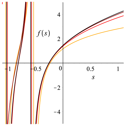
Figure 3: Convergence of the scaled generating function $G(z,q)$ to the scaling function $f(s)$ for $q=0.99$, $0.9999$, and $0.999999$. Numerical evaluation of $G(z,q)$ has been done using the continued fraction representation (3.7).

Much work has been done on the computation of the asymptotics for $q$-series such as those involved here [17]. In the vicinity of $q=1$ and $z=z_{c}(1)=1/4$, one can show convergence of suitably scaled generating function. More precisely, one finds that the limit

$$f(s)=\lim_{q\to 1^{-}}-\left((1-q)^{-1/3}G(1/4-s(1-q)^{2/3},q)-2\right)$$ (3.11)

exists and is equal to the scaling function

$$f(s)=-2\frac{\mbox{\rm Ai}^{\prime}(4s)}{\mbox{\rm Ai}(4s)}$$ (3.12)

The convergence to the scaling function is shown in Figure 3.

3.2 Pressure profiles

We now consider the profile of the pressure for finite $N$. In Figure 4 we show pressure profiles as a function of $x=m/N$ for three different values of $q$ with positive, zero, and negative osmotic pressures, and for lengths $N=50$, $100$, and $200$.

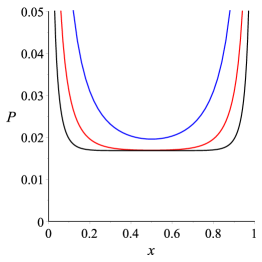
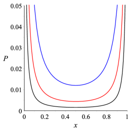
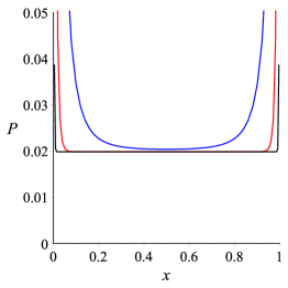
Figure 4: Pressure profiles for $q=0.98$ (left), $1.00$ (center), and $1.02$ (right) and lengths $N=50$, $100$, and $200$, from top to bottom.

We see that the pressure converges to a non-zero bulk pressure when the osmotic pressure is non-zero. For $q=1$, one can compare the finite-size data shown in this figure to the exactly known scaled profile shown in Figure 1. Moreover, closer inspection shows that the rate of convergence is significantly different for positive and negative osmotic pressure. As we know, for $q=1$ the bulk pressure is zero, and convergence obeys the power law $N^{-3/2}$. For $q\neq 1$, the rate of convergence to the bulk pressure is exponential in $N$ and $N^{2}$ for $q<1$ and $q>1$, respectively, as can be seen in Figure 5.

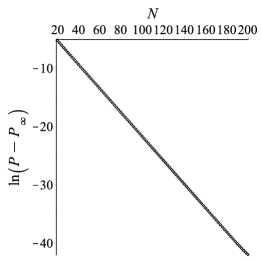
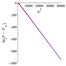
Figure 5: The rates of approach to the bulk pressure, calculated via the pressure at the centre of the vesicle for $q=0.9$ (left) and $q=1.1$ (right). Clearly the convergence is exponential in $N$ for $q<1$ and exponential in $N^{2}$ for $q>1$. The straight line (right) is our theoretical prediction.

One can derive these results in the following way. Convergence to the thermodynamic limit is encoded in the singularity structure of the generating function. For $q<1$, the leading singularity of the generating function is an isolated simple pole, and the finite-size corrections to scaling are therefore exponential, with the rate of convergence given by the ratio between the magnitudes of the leading singularity and the sub-leading one. A closer analysis reveals that the rate depends on the value $x=m/N$ as

$$P_{N}^{(m)}(q)\sim-\log(1-\rho(q))+\log q+O(e^{-D\min(x,1-x)N})\;,$$ (3.13)

where $D$ does not depend on the value of $x$. The singularity structure can also be seen in Figure 3 for negative values of the scaling parameter $s$.

For $q>1$, it is easier to argue directly via the partition functions. For positive osmotic pressure, configurations with large area dominate, and using arguments in [18] one can deduce that

$$Z_{N}(q)\sim\frac{1}{(q^{-1};q^{-1})_{\infty}}q^{\binom{N}{2}}$$ (3.14)

where $(t;q)_{\infty}=\prod_{k=0}^{\infty}(1-tq^{k})$ is again a $q$-product. The appearance of the factor $1/(q^{-1};q^{-1})_{\infty}$ is due to fluctuations around configurations of maximal area.

Substituting this into Eqn. (2.4) shows that

$$P_{N}^{(m)}(q)\sim\log q+\frac{1}{(q^{-1};q^{-1})_{\infty}}q^{-m(N-m)}=\log q+\frac{1}{(q^{-1};q^{-1})_{\infty}}q^{-x(1-x)N^{2}}\;.$$ (3.15)

Note that the decay rate depends on the value of $x=m/N$.

3.3 Bulk pressure

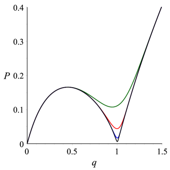
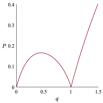
Figure 6: A plot of the pressure at the centre of the vesicle against $q$ for vesicle lengths $10$, $20$, $40$ and $80$, from top to bottom (left) and of the thermodynamic limit bulk pressure of the vesicle against $q$ (right).

We now turn to the consideration of the pressure in the centre of the vesicle, so as to consider the bulk pressure. Using our results above, we already know that for $q>1$ the bulk pressure is given by $\log q$. In Figure 6 on the left we have used the recursion (3.1) to calculate the pressure at the centre of the vesicle as a function of $q$ for $N=10$, $20$, $40$, and $80$. One can see that the convergence to a limit is slowest around $q=1$, which of course aligns with our predictions above for the rates of convergence in the different regimes.

We have now used the continued fraction expansion (3.7) to numerically estimate the thermodynamic limit bulk pressure as a function of $q$, shown on the right in Figure 6. It should be clear that the finite-size curves approach the curve shown here in the limit of large $N$. It is interesting to see the competition of the osmotic pressure and the entropic pressure for $q<1$.

Clearly the limiting behaviour of the pressure for $q>1$ is $P(q)\sim q-1$ as $q\to 1^{+}$. Extracting the limiting behaviour of the pressure for $q<1$ is considerably more difficult. A calculation starts by considering that from Equations (3.6) and (3.8) we find that the critical fugacity $z_{c}=z_{c}(q;\kappa)$ satisfies

$$G(z_{c},q)=\frac{\kappa}{\kappa-1}\;.$$ (3.16)

Differentiating this expression with respect to $\kappa$ allows us to write the density $\rho(q)$ in terms of the generating function as

$$\rho(q)=\frac{G(z_{c},q)(G(z_{c},q)-1)}{z\frac{\partial}{\partial z_{c}}G(z_{c},q)}\;.$$ (3.17)

Utilising the scaling form (3.11) now shows that $\rho(q)\sim 2(1-q)$ as $q\to 1^{-}$ and hence $P(q)\sim 1-q$. Put together, this implies that

$$P(q)\sim|1-q|\quad\text{as $q\to 1$.}$$ (3.18)

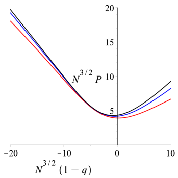
Figure 7: An estimate of the finite-size scaling function for the pressure, using $N=40$, $80$, and $160$, from bottom to top.

The existence of the scaling function $f(s)$ in the variable $s=(1/4-z)/(1-q)^{2/3}$ implies by standard Laplace transform that there should be a finite-size scaling form for the pressure in the variable $t=N^{3/2}(1-q)$. Hence we define the scaling function

$$g(t)=\lim\limits_{N\to\infty}N^{3/2}P_{N}^{(N/2)}(1-tN^{-3/2})\;.$$ (3.19)

In Figure 7, we numerically estimate the scaling function $g(t)$ for a range of $t$. Asymptotic matching with (3.18) requires that $g(t)\to|t|$ for $t\to\pm\infty$. We note the convergence to the scaling function is poor for $q>1$, which arises because of the unusually differing rates of convergence to the thermodynamic limit in the two regimes.

References

- [1] Bijsterbosch H, de Haan V, de Graaf A, Mellema M, Leermakers F, Stuart M C and vanWell A A 1995 Langmuir 11 4467–4473
- [2] Carignano M and Szleifer I 1995 Macromolecules 28
- [3] Currie E P K, Norde W and Stuart M A C 2003 Advances in Colloid and Interface Science 100102 205–265
- [4] Jensen I, Dantas W G, Marques C M and Stilck J F 2013 J. Phys. A. 46 115004
- [5] Janse van Rensburg E J and Prellberg T 2013 The pressure exerted by adsorbing directed lattice paths and staircase polygons
- [6] Gassoumov F and Janse van Rensburg E J 2013 J. Stat. Mech.
- [7] Leibler S, Singh R R P and Fisher M E 1987 Phys. Rev. Lett 59 1989
- [8] Brak R and Guttmann A J 1990 J. Phys A. 23 4581
- [9] Fisher M E, Guttmann A J and Whittington S 1991 J. Phys. A 24 3095
- [10] Owczarek A L and Prellberg T 1993 J. Stat. Phys. 70 1175–1194
- [11] Brak R, Owczarek A L and Prellberg T 1994 J. Stat. Phys. 76 1101–1128
- [12] Prellberg T and Owczarek A L 1995 J. Stat. Phys. 80 755–779
- [13] Janse van Rensburg E J 2000 The Statistical Mechanics of Interacting Walks, Polygons, Animals and Vesicles (Oxford: Oxford University Press)
- [14] Owczarek A and Prellberg T 2010 J. Stat. Mech.: Theor. Exp. P08015 (13pp)
- [15] Owczarek A and Prellberg T 2012 J. Phys. A: Math. Theor. 45 395001 (10pp)
- [16] Flajolet P and Sedgewick A 2009 Analytic Combinatorics (Cambridge: Cambridge University Press)
- [17] Prellberg T and Brak R 1995 J. Stat. Phys. 78 701–730
- [18] Prellberg T and Owczarek A L 1999 Commun. Math. Phys. 201 493–505