Entanglement of three cavity fields via resonant interactions with dressed three-level atoms

Abstract

In this paper we show that three cavity fields can be entangled when they are tuned on resonance with an ensemble of dressed three-level atoms. The master equation for the three cavity modes is derived by using atomic dressed states and the inseparability of the three output cavity modes is described by using a sufficient criterion proposed by van Loock and Furusawa. The physical cause is the atomic coherence effects, by which the quantum correlations are created in the field dynamics.

Keywords: continuous-variable entanglement, output tripartite entanglement, atomic coherence

I Introduction

Atomic coherence lies in the center of many novel effects in quantum optics and laser physics. Electromagnetically induced transparency [1,2], coherent population trapping [2], Hanel-effect laser [3] and quantum beat laser [4] are such examples. Besides these, the correlation between the photons can also be induced by atomic coherence [5-12]. One such example is the generation of squeezed light in a three-level cascade laser using atomic coherence [5-8]. The atomic coherence can be created by preparing the atoms initially in a coherent superposition state of the two states which are dipole-forbidden [5-8] or driving the two states by a strong coherent field [9-11] or Raman coupling the two states through the third auxiliary atomic states [12]. For two-photon correlated-spontaneous-emission laser with injected atomic coherence, it exhibits complete spontaneous-emission noise quenching and phase squeezing simultaneously [5]. It has also been pointed out that atomic coherence in a two-photon correlated emission laser system can be used to generate a macroscopic two-mode entangled state and this system can be treated as an entanglement amplifier [12].

Recently, the topic of continuous-variable entanglement has attracted much attention as it is the base of all branches of quantum information and communication protocols [13]. Among various entanglement generation schemes, entanglement induced by atomic coherence has been extensively researched [14-16]. For a nondegenerate three-level cascade laser with a subthreshold nondegenerate parametric oscillator coupled to a vacuum reservoir, the entanglement and squeezing for the two cavity modes in this combined system is induced by the injected atomic coherence [14]. In a two-mode single-atom laser with the atomic coherence exhibited by two classical laser fields, entanglement between two field modes is demonstrated [15]. Later, it was shown that in a three-level $\Lambda$ or V atomic system with two classical driving fields and two cavity modes coupling corresponding transitions, by exploring the two-channel interaction mechanism and using the squeeze-transformed modes, continuous-variable entanglement between the two modes is obtained and the best achievable entangled state approaches the original EPR state [16]. The above work has mainly been confined to two-partite systems.

With the progress in continuous-variable entanglement, the generation of more than two partite entanglement has been paid much attention as it may be the key ingredient for advanced multiparty quantum communication such as quantum teleportation network [17], telecloning [18] and controlled dense coding [19]. Among various generation schemes for tripartite systems, few work has been done to generate tripartite entanglement using atomic coherence. Most recently, a scheme to generate three-mode-entangled light fields via the interaction between the four-level atoms and the cavity has been proposed [20]. Three cavity modes are generated through three successive transitions in the four-level cascade atoms. In addition to the cavity modes, two strong classical fields drive a pair of two-photon transitions in the four-level atoms. They show that the entanglement could only be obtained in a short time as all the mean photons are amplified as time elapses. Thus at steady time, the entanglement does not exist.

In this paper, we present a scheme to generate tripartite entanglement for three cavity modes via the interaction for the three-level lambda atoms with the three cavity modes and two classical fields. As the classical fields are strong, the effective interaction is resonant interaction in the dressed-state picture. We deduce the master equation of the three cavity modes by means of the atomic dressed states and linear theory. The sufficient inseparability criterion for continuous-variable entanglement is used to demonstrate the entanglement properties of the three cavity modes and the results show that our system can be used as a source to generate tripartite entangled light even at steady state.

It is should be noted that, up to now many schemes have been proposed to generate tripartite entanglement using linear optics or nonlinearities [17, 21-26]. It was theoretically predicted that using single-mode squeezed state and linear optics, a truly N-partite entangled state can be generated [17]. Later, a continuous-variable tripartite entangled state was experimental realized by combing three independent squeezed vacuum states [21]. At first, the production of continuous-variable tripartite entanglement was presented by mixing squeezed beams on unbalanced beamsplitters [21,22]. Recently, generation of tripartite entanglement are focused on using cascade nonlinear interaction in an optical cavity [23-25] or in a quasiperiodic superlattice [26]. Among the latter are systems using parametric down-conversion with sum frequency generation [23,25,26] or using single nonlinearity [24]. During these nonlinear processes, the cavity modes couple with each other directly. As these nonlinear processes are related to the higher-order polarization, the efficiency of these processes are relatively small compared with the processes related to linear polarization. In this way, these nonlinear processes are not the best choice for the generation of high efficiency tripartite entangled states.

Compared with the schemes based on the nonlinear processes [23-26], our scheme is more effective as the generation process is resonant interaction in the dressed states and it is only related to linear polarization. What’s more, the linear process provides much more parameters to choose than that of the nonlinear processes, as the atomic parameters can be varied. Compared with the scheme in Ref. [20], our scheme can provide steady state tripartite entanglement while the entanglement produced in scheme [20] is just kept in a quite limited time. And in Ref. [20], they use four-level cascade atomic system and the effective processes in the dressed states of the driving fields are all two-photon transitions. High excited states are involved in their scheme. In our scheme we use three-level $\Lambda$ atomic system, and the effective processes in the dressed states of the driving fields are all single-photon transitions. When we take into the account of the atomic spontaneous emission, their schemes seems to have more obstacles than ours.

The paper is organized as follows. In Sec. II, we discuss the essential ingredients of the model and deduce the density-matrix equation for the cavity fields in a dressed-state picture. In Sec. III, we present the output correlation spectra by solving the equations of the cavity fields and analyze the output tripartite continuous-variable entanglement characteristics by using a sufficient criterion proposed by van Loock and Furusawa. In Sec. IV, we give a brief conclusion.

II Model and equation

We consider $N$ three-level lambda-type atoms in a three-mode cavity as shown in Fig. 1(a). Two laser fields of frequencies $\omega_{l1,l2}$ drive the transitions $|1,2\rangle\leftrightarrow$ $|3\rangle$, respectively. Two cavity modes $a_{1,2}$ of frequencies $\omega_{c1,c2}$ couple the atomic transition $|1\rangle\leftrightarrow$ $|3\rangle$, while the cavity mode $a_{3}$ with frequency $\omega_{c3}$ couples the transition $|2\rangle\leftrightarrow$ $|3\rangle$. $\gamma_{l}$ ($l=1,2$) are the atomic decay rates from level $|3\rangle$ to levels $|1,2\rangle$ and $\kappa_{l}$ ($l=1,2,3$) are the cavity loss rates. For simplicity, we assume that $\gamma_{1}=\gamma_{2}=\gamma$ and $\kappa_{1}=\kappa_{2}=\kappa_{3}=\kappa$. The three cavity modes are assumed to be in their vacuum state initially. In the frame of the frequencies of the laser fields and under the dipole and the rotating-wave approximations, the total Hamiltonian is

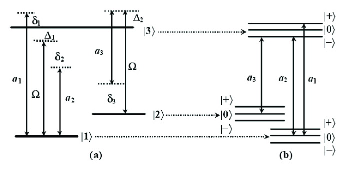
Figure 1: (a) Atomic energy level scheme and the coupling of the cavity fields and the classic fields. (b) Equivalent resonant transitions in the picture dressed by the classical fields.

$$H = H_{1}+H_{2}+H_{3},$$

$$H_{1} = \sum_{j=1}^{3}\hbar\delta_{j}a_{j}^{\dagger}a_{j},$$

$$H_{2} = -\hbar\Delta\left(\sigma_{11}-\sigma_{22}\right)+\hbar\Omega\left(\sigma_{31}+\sigma_{32}+H.c.\right),$$ (1)

$$H_{3} = i\hbar g\left(a_{1}\sigma_{31}+a_{2}\sigma_{31}+a_{3}\sigma_{32}\right)+H.c.,$$

H.c. symbols the Hermitian conjugate. $H_{1}$ denotes the free energy for three cavity fields, $H_{2}$ describes the interaction of the laser fields with the atoms, and $H_{3}$ indicates the interaction of the cavity fields with the atoms. $\sigma_{jk}=|j\rangle\langle k|$ ($j,k=1,2,3$) are atomic dipole operators for $j\neq k$ and atomic projection operators for $j=k$. The cavity detunings are defined as $\delta_{j}=\omega_{cj}-\omega_{l1}$ ($j=1,2$), and $\delta_{3}=\omega_{c3}-\omega_{l2}$. The detunings of the laser fields are defined as $\Delta_{j}=\omega_{3j}-\omega_{lj}$ ($j=1,2$), where $\omega_{31}$ and $\omega_{32}$ are the resonance frequencies of transitions $|1,2\rangle\leftrightarrow$ $|3\rangle$. We have assumed equal coupling coefficients $g$ for three cavity modes, equal Rabi frequency $\Omega$ for the two laser fields, and opposite detunings of the two laser fields $\Delta_{1}=-\Delta_{2}=\Delta$.

We assume that the laser fields are much stronger than the cavity fields, i.e., $\Omega\gg g\langle a_{l}\rangle$, ($l=1,2,3)$. The laser fields can be viewed as dressing fields for the atoms. Therefore, by diagonalizing the Hamiltonian $H_{2}$, we find the so-called semiclassical dressed states as

$$|0\rangle = -\frac{c}{\sqrt{2}}|1\rangle+\frac{c}{\sqrt{2}}|2\rangle+s|3\rangle,$$

$$|+\rangle = \frac{1+s}{2}|1\rangle+\frac{1-s}{2}|2\rangle+\frac{c}{\sqrt{2}}|3\rangle,$$ (2)

$$|-\rangle = \frac{1-s}{2}|1\rangle+\frac{1+s}{2}|2\rangle-\frac{c}{\sqrt{2}}|3\rangle,$$

where $c=\frac{\sqrt{2}\Omega}{d}$, $s=-\frac{\Delta}{d}$, and $d=\sqrt{\Delta^{2}+2\Omega^{2}}$.

Now, we use the Hamiltonian $H_{0}=\hbar d\left(\sigma_{++}-\sigma_{--}\right)+H_{1}$ to perform the unitary dressing transformation. By choosing the cavity detunings as $\delta_{1}=d=-\delta_{2}=-\delta_{3}$, and neglecting the fast-oscillating terms such as $e^{\pm i2dt}$, we obtain the resonant interaction Hamiltonian as

$$V=ig\hbar\left(c_{3}a_{1}^{\dagger}+c_{2}a_{2}+c_{1}a_{3}\right)\sigma_{0+}+ig\hbar\left(c_{1}a_{1}-c_{3}a_{2}^{\dagger}+c_{3}a_{3}^{\dagger}\right)\sigma_{0-}+H.c.,$$ (3)

where $c_{1}=\frac{1}{2}s(1-s)$, $c_{2}=\frac{1}{2}s(1+s)$, and $c_{3}=\frac{1}{2}c^{2}$. The resonant transitions in the dressed states are shown in Fig. 1(b).

The master equation for the cavity modes is obtained by using the usual approach [2], starting from $\frac{d}{dt}\rho=-\frac{i}{\hbar}\left[V,\rho\right]{\cal+L}_{a}\rho+{\cal L}_{c}\rho$, where ${\cal L}_{c}\rho=\frac{{}_{\kappa}}{2}\sum_{l=1}^{3}\left(2a_{l}\rho a_{l}^{\dagger}-a_{l}^{\dagger}a_{l}\rho-\rho a_{l}^{\dagger}a_{l}\right)$ and ${\cal L}_{a}\rho$ describes the atomic decay in the dressed states picture and its expression is very complicated. The detailed form of atomic decay term ${\cal L}_{a}\rho$ is given in Appendix A. The master equation for the cavity modes is obtained by tracing out the atomic states, which gives $\frac{d}{dt}\rho_{c}=g\left(c_{3}a_{1}^{\dagger}+c_{2}a_{2}+c_{1}a_{3}\right)\rho_{+0}+g\left(c_{1}a_{1}-c_{3}a_{2}^{\dagger}+c_{3}a_{3}^{\dagger}\right)\rho_{-0}+H.c$, where $\rho_{jk}=tr_{atom}(\sigma_{kj}\rho)$ ($j,k=0,+,-$). As the atomic variables vary much faster than the cavity fields, it is possible to express $\rho_{jk}=tr_{atom}(\sigma_{kj}\rho)$ ($jk=+0,-0,0+,0-$) in terms of $\rho_{c}$, $a_{l}$ and $a_{l}^{\dagger}$ ($l=$1-3) from the quasi-steady-state solution of the coupled equations for $\rho_{jk}=tr_{atom}(\sigma_{kj}\rho)$ ($jk=+0,-0,0+,0-$). By using $\rho_{jj}\simeq\rho_{jj}^{s}\rho_{c}$ ($j=0,+,-$) and $\rho_{+-}^{s}\simeq 0$, where “s” implies the steady-state solutions of the density matrix equations in the dressed state picture without the quantum fields $a_{l}$ and $a_{l}^{\dagger}$ ($l=$1-3). The steady state populations is obtained as $\rho_{00}^{s}=\frac{c^{4}}{1+3s^{4}}$ and $\rho_{++}^{s}=\rho_{--}^{s}=\frac{s^{2}\left(1+s^{2}\right)}{1+3s^{4}}$. The master equation for the cavity modes is obtained as

$$\frac{d}{dt}\rho_{c} = \sum_{l=1}^{3}\left\{A_{ll}\left[a_{l}^{\dagger},\rho_{c}a_{l}\right]-\left(B_{ll}+\frac{\kappa_{l}}{2}\right)\left[a_{l}^{\dagger},a_{l}\rho_{c}\right]\right\}$$

$$+\sum_{l=2}^{3}\left\{A_{1l}\left[a_{1}^{\dagger},\rho_{c}a_{l}^{\dagger}\right]-B_{1l}\left[a_{1}^{\dagger},a_{l}^{\dagger}\rho_{c}\right]+A_{l1}\left[a_{l}^{\dagger},\rho_{c}a_{l}^{\dagger}\right]-B_{l1}\left[a_{l}^{\dagger},a_{1}^{\dagger}\rho_{c}\right]\right\}$$

$$+\sum_{l,k=2;l\neq k}^{3}\left\{A_{lk}\left[a_{l}^{\dagger},\rho_{c}a_{k}\right]-B_{lk}\left[a_{l}^{\dagger},a_{k}\rho_{c}\right]\right\}+H.c..$$

The explicit expressions for $A_{lk}$ and $B_{lk}$ ($l,k=1,2,3$) are given in Appendix B. Here the terms $A_{ll}$ ($l$=1-3) and $B_{ll}$ ($l$=1-3) represent the gain term and the absorption of mode $a_{l}$, respectively. And the terms $A_{lk}$ and $B_{lk}$ ($l\neq k$) represent the coupling between the two modes $a_{l}$ and $a_{k}$, and we will show that these quantities are responsible for entanglement among three cavity fields. It is easy to see that without these coupling terms between different cavity fields, the quantum correlation can not be introduced among the three cavity modes. Thus entanglement among the three cavity fields is attributed to the atomic coherence created through the interaction between the fields and the atoms.

III Correlation spectra

The master equation (4) enables us to derive equations of motion for the cavity modes:

$$\tau\frac{d}{dt}a_{1}^{\dagger} = \left(A_{11}-B_{11}-\frac{\kappa_{1}}{2}\right)a_{1}^{\dagger}+\left(A_{12}-B_{12}\right)a_{2}+\left(A_{13}-B_{13}\right)a_{3}+\sqrt{\kappa_{1}}a_{1}^{\dagger in},$$

$$\tau\frac{d}{dt}a_{2} = \left(A_{21}-B_{21}\right)a_{1}^{\dagger}+\left(A_{22}-B_{22}-\frac{\kappa_{2}}{2}\right)a_{2}+\left(A_{23}-B_{23}\right)a_{3}+\sqrt{\kappa_{2}}a_{2}^{in},$$ (5)

$$\tau\frac{d}{dt}a_{3} = \left(A_{31}-B_{31}\right)a_{1}^{\dagger}+\left(A_{32}-B_{32}\right)a_{2}+\left(A_{33}-B_{33}-\frac{\kappa_{3}}{2}\right)a_{3}+\sqrt{\kappa_{3}}a_{3}^{in},$$

where $\tau$ is the round-trip time of light in the cavity and assumed to be the same for three cavity modes. $a_{j}^{in}$ and $a_{j}^{\dagger in}$ ($j=$1-3) are annihilation and creation operators of the input fields to the cavity. This is a set of linear equations. In order to solve this equation, we use the Fourier transformation and the boundary conditions at the mirror between the output quantities and the input quantities $a_{j}^{in}+a_{j}^{out}=\sqrt{\kappa_{j}}a_{j}$ ($j=$1-3) to obtain the equation in the frequency domain as

$$a^{out}\left(\omega\right)=-\left(I+BD_{0}^{-1}B\right)a^{in}\left(\omega\right),$$ (6)

where

$$a^{out}\left(\omega\right)=\left(a_{1}^{\dagger out}\left(-\omega\right),a_{2}^{out}\left(\omega\right),a_{3}^{out}\left(\omega\right)\right)^{T},$$

(7)

$$D_{0}=\left(\begin{array}[]{ccc}A_{11}-B_{11}-\frac{\kappa_{1}}{2}-i\omega\tau&A_{12}-B_{12}&A_{13}-B_{13}\\ A_{21}-B_{21}&A_{22}-B_{22}-\frac{\kappa_{2}}{2}-i\omega\tau&A_{23}-B_{23}\\ A_{31}-B_{31}&A_{32}-B_{32}&A_{33}-B_{33}-\frac{\kappa_{3}}{2}-i\omega\tau\end{array}\right),$$ (8)

$$B=\left(\begin{array}[]{lll}\sqrt{\kappa_{1}}&0&0\\ 0&\sqrt{\kappa_{2}}&0\\ 0&0&\sqrt{\kappa_{3}}\end{array}\right),\text{\qquad}I=\left(\begin{array}[]{lll}1&0&0\\ 0&1&0\\ 0&0&1\end{array}\right).$$ (9)

where T symbols the matrix transpose.

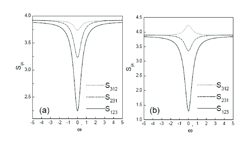
Figure 2: The quantum correlations spectra $S_{123}^{out}\left(\omega^{\prime}\right)$, $S_{231}^{out}\left(\omega^{\prime}\right)$ and $S_{312}^{out}\left(\omega^{\prime}\right)$ versus the normalized analyzing frequency $\omega^{\prime}$ are plotted for (a) $\Delta=5$ and (b) $\Delta=10$ by solid, dashed and dotted line, respectively. The other parameters are $\Omega=35$, $g^{2}N=10$, $\gamma=1$ and $\kappa=0.1$.

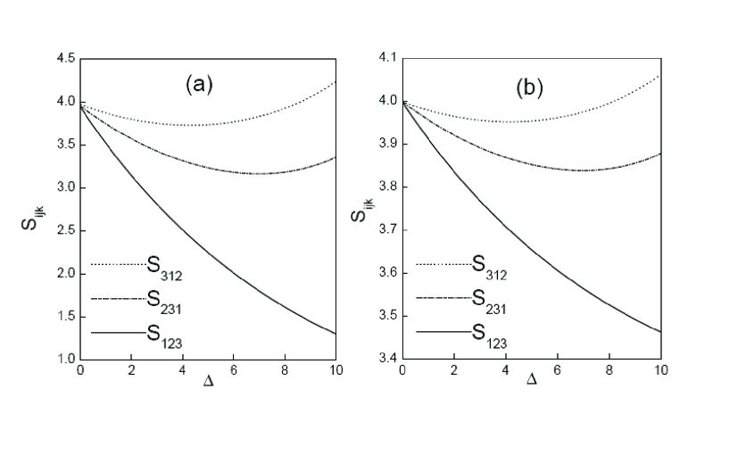
Figure 3: The quantum correlations spectra $S_{123}^{out}\left(\omega^{\prime}\right)$, $S_{231}^{out}\left(\omega^{\prime}\right)$ and $S_{312}^{out}\left(\omega^{\prime}\right)$ versus the detuning $\Delta$ for (a) $\omega^{\prime}=0$ and (b) $\omega^{\prime}=1.0$ by solid, dashed and dotted line, respectively. The other parameters are the same as those in Fig. 2.

In order to study the entanglement properties of output cavity modes, we need to use quadrature amplitude and phase operators defined by

$$X_{j}^{out} = a_{j}^{out}\left(\omega\right)+a_{j}^{\dagger out}\left(-\omega\right),$$

$$Y_{j}^{out} = -i\left[a_{j}^{out}\left(\omega\right)-a_{j}^{\dagger out}\left(-\omega\right)\right],$$ (10)

Using Eq. (6) and $X_{j}^{in}=a_{j}^{in}\left(\omega\right)+a_{j}^{\dagger in}\left(-\omega\right)$, $Y_{j}^{in}=-i\left[a_{j}^{in}\left(\omega\right)+a_{j}^{\dagger in}\left(-\omega\right)\right]$, we can obtain the relationships between the input fields and the output fields as

(13)

(16)

(19)

where we have defined the normalized analyzing frequency $\omega^{\prime}=\omega\tau/\kappa$. The explicit expressions for $D_{jk}$ ($j,k$=1-3) are presented in Appendix C.

The presence of entanglement between the three cavity modes can be investigated using the sufficient criterion for continuous-variable tripartite system proposed by van Loock and Furusawa [27]. The sufficient inseparability criterion for continuous variable tripartite entanglement is that if any one of the following inequalities is satisfied, genuine tripartite entanglement is demonstrated. The inequalities are

$$S_{123} = V\left[X_{1}+\left(X_{2}+X_{3}\right)/\sqrt{2}\right]+V\left[Y_{1}-\left(Y_{2}+Y_{3}\right)/\sqrt{2}\right]<4,$$

$$S_{231} = V\left[X_{2}+\left(X_{3}+X_{1}\right)/\sqrt{2}\right]+V\left[Y_{2}-\left(Y_{3}+Y_{1}\right)/\sqrt{2}\right]<4,$$ (20)

$$S_{312} = V\left[X_{3}+\left(X_{1}+X_{2}\right)/\sqrt{2}\right]+V\left[Y_{3}-\left(Y_{1}+Y_{2}\right)/\sqrt{2}\right]<4,$$

where $V\left(A\right)=<A^{2}>-<A>^{2}$. From the above definition, the correlation spectra of the quadratures of three output cavity fields are obtained as

$$S_{123}^{out}\left(\omega^{\prime}\right) = |\sqrt{2}D_{11}-D_{21}-D_{31}|^{2}+|\sqrt{2}D_{12}-D_{22}-D_{32}|^{2}+|\sqrt{2}D_{13}-D_{23}-D_{33}|^{2},$$

$$S_{231}^{out}\left(\omega^{\prime}\right) = \frac{1}{2}\left(|\sqrt{2}D_{21}-D_{11}-D_{31}|^{2}+|\sqrt{2}D_{22}-D_{12}-D_{32}|^{2}+|\sqrt{2}D_{23}-D_{13}-D_{33}|^{2}\right)$$ (21)

$$+\frac{1}{2}\left(|\sqrt{2}D_{21}-D_{11}+D_{31}|^{2}+|\sqrt{2}D_{22}-D_{12}+D_{32}|^{2}+|\sqrt{2}D_{23}-D_{13}+D_{33}|^{2}\right),$$

$$S_{312}^{out}\left(\omega^{\prime}\right) = \frac{1}{2}\left(|\sqrt{2}D_{31}-D_{11}-D_{21}|^{2}+|\sqrt{2}D_{32}-D_{12}-D_{22}|^{2}+|\sqrt{2}D_{33}-D_{13}-D_{23}|^{2}\right)$$

$$+\frac{1}{2}\left(|\sqrt{2}D_{31}+D_{11}-D_{21}|^{2}+|\sqrt{2}D_{32}-D_{12}+D_{22}|^{2}+|\sqrt{2}D_{33}-D_{13}+D_{23}|^{2}\right).$$

The quantum correlations spectra $S_{123}^{out}\left(\omega^{\prime}\right)$, $S_{231}^{out}\left(\omega^{\prime}\right)$ and $S_{312}^{out}\left(\omega^{\prime}\right)$ for three output cavity fields described in Eq. (13) versus the normalized analyzing frequency $\omega^{\prime}$ are plotted in Fig. $2$ for (a) $\Delta=5$ and (b) $\Delta=10$ by solid, dashed and dotted line, respectively. The other parameters are $\Omega=35$, $g^{2}N=10$, $\gamma=1$ and $\kappa=0.1$. The satisfaction of one of the three inequalities $S_{123}^{out}\left(\omega^{\prime}\right)<4$, $S_{231}^{out}\left(\omega^{\prime}\right)<4$ and $S_{312}^{out}\left(\omega^{\prime}\right)<4$ is sufficient to demonstrate genuine tripartite entanglement. In order to analyze the entanglement properties of the three cavity modes, we present all three correlations $S_{ijk}^{out}\left(\omega^{\prime}\right)$ and find that the indices of the three cavity modes are crucial. When the cavity modes are symmetric, the indices of the cavity modes are not important as the three correlations give the same result. But when the cavity modes are asymmetric, the indices are crucial in that the three correlations will give different results. As shown in Fig. 2(a), all three correlations are below 4 in a wide frequency range thus all three inequalities are satisfied. So the three output cavity modes are entangled. Among the three correlations, $S_{123}^{out}\left(\omega^{\prime}\right)$ gives the minimum values with the same parameters. When the inequalities are satisfied, the smaller the values of correlations are the larger the correlation degree. When we increase the detuning $\Delta$ to $10$ and keep other parameters unchanged as shown in Fig. 2(b), correlations $S_{123}^{out}\left(\omega^{\prime}\right)$ and $S_{231}^{out}\left(\omega^{\prime}\right)$ are always below $4$ in a wide frequency range while the correlation $S_{312}^{out}\left(\omega^{\prime}\right)$ is larger than $4$ in a frequency zone around the central analyzing frequency $\omega^{\prime}=0$. Thus tripartite entanglement is also demonstrated between the three output cavity modes. Compared with Fig. 2(a), the minimum value of $S_{123}^{out}\left(\omega^{\prime}\right)$ is smaller, which means that the correlation degree is also increased with the detuning. For both cases, we also see that the large correlation can be obtained at low analyzing frequency $\omega^{\prime}$.

In Fig. $3$, we plot $S_{123}^{out}\left(\omega^{\prime}\right)$, $S_{231}^{out}\left(\omega^{\prime}\right)$ and $S_{312}^{out}\left(\omega^{\prime}\right)$ as a function of detuning $\Delta$ for (a) $\omega^{\prime}=0$ and (b) $\omega^{\prime}=1.0$ by solid, dashed and dotted line, respectively. The remain parameters are the same as those in Fig. 2. We also see that the correlation $S_{123}^{out}\left(\omega^{\prime}\right)$ gives the minimum values with the same parameters. It is seen from Fig. 3(a) and 3(b) that, correlations $S_{123}^{out}\left(\omega^{\prime}\right)$ and $S_{231}^{out}\left(\omega^{\prime}\right)$ always satisfy the inequalities while $S_{312}^{out}\left(\omega^{\prime}\right)$ only satisfy the inequality in a small frequency range. Thus tripartite entanglement between the three output cavity modes is demonstrated again. It is worthwhile to point out that when the analyzing frequency $\omega^{\prime}=0$, the system reaches its steady state. Thus at steady state, we can also obtain entangled tripartite light. This is in contrast with the results in Ref. [20], where the entanglement between the three cavity modes is time dependent. In that case all the mean photon numbers are amplified as time increases. Thus, the entanglement for three cavity modes can not be kept for a long time. And among the three correlations, $S_{123}^{out}\left(\omega^{\prime}\right)$ decreases with the increasing detuning, while correlations $S_{231}^{out}\left(\omega^{\prime}\right)$ and $S_{312}^{out}\left(\omega^{\prime}\right)$ first decrease than increase with increasing detuning. So correlation $S_{123}^{out}\left(\omega^{\prime}\right)$ is the best choice when we investigate the entanglement properties of the three cavity modes. Compared with Fig. 3(a) and 3(b), we find that the minimal values of correlations in Fig. 3(a) are smaller than those in Fig. 3(b). This indicates that the correlation degree is large when the analyzing frequency $\omega^{\prime}$ is small.

IV Conclusion

In conclusion, we have examined the entanglement properties of three cavity modes interacting with three-level $\Lambda$ atomic system coupled by two extra classical fields. As the classical fields are stronger than the cavity fields, we adopt the dressed-atom approach to calculate the equation for the cavity fields. After tracing out the atomic variables, we obtain the master equation of the cavity modes and analyze the entanglement properties of the output fields. The tripartite entanglement of the three output fields is demonstrated theoretically by a sufficient inseparability criterion and the entanglement characteristics are presented. This scheme of three-mode continuous variable entanglement generation using atomic coherence is useful in quantum information processing.

Acknowledgments

This work is supported by the Scientific Research Plan of the Provincial Education Department in Hubei (Grant No. Q20101304) and NSFC under Grant No. 11147153.

Appendix A

In this Appendix, we present the atomic decay term in terms of the dressed atomic states as

$${\cal L}_{a}\rho = \sum_{j,k=0,+,-;j\neq k}\left({\cal L}_{jk}^{kj}\rho+{\cal L}_{ph}^{kj}\rho\right)+\sum_{j,k=+,-;j\neq k}{\cal L}_{in}^{kj}\rho,$$

$${\cal L}_{jk}^{kj}\rho = \frac{{}_{\gamma_{jk}}}{2}\left(2\sigma_{p}^{kj}\rho\sigma_{p}^{kj}-\sigma_{p}^{kj}\sigma_{p}^{kj}\rho-\rho\sigma_{p}^{kj}\sigma_{p}^{kj}\right),$$

$${\cal L}_{ph}^{kj}\rho = \epsilon_{kj}\frac{{}_{\gamma_{ph}^{kj}}}{4}\left(2\sigma_{jk}\rho\sigma_{kj}-\sigma_{kj}\sigma_{jk}\rho-\rho\sigma_{kj}\sigma_{jk}\right),$$ ()

$$\sigma_{p}^{kj} = \sigma_{kk}-\sigma_{jj},$$

$${\cal L}_{in}^{kj}\rho = \gamma_{c}\left(\sigma_{j0}\rho\sigma_{k0}+\sigma_{0j}\rho\sigma_{0k}\right),$$

with $\epsilon_{kj}=1$, for $k,j=0+,0-,+-$, otherwise $\epsilon_{kj}=0$. The parameters in the above equations are

$$\gamma_{+-} = \gamma_{-+}=\frac{\gamma}{4}c^{2}\left(1+s^{2}\right),$$

$$\gamma_{+0} = \gamma_{-0}=\frac{\gamma}{2}s^{2}\left(1+s^{2}\right),$$

$$\gamma_{0+} = \gamma_{0-}=\frac{\gamma}{2}c^{4},\gamma_{c}=\frac{\gamma}{2}c^{2}s^{2},$$ ()

$$\gamma_{ph}^{0+} = {\cal\gamma}_{ph}^{0-}=\gamma c^{2}s^{2},\gamma_{ph}^{+-}=\frac{\gamma}{2}c^{4}.$$

Appendix B

In this appendix, we present the explicit expressions for the coefficients $A_{jk}$ and $B_{jk}$ ($j,k=$1-3) in the equation of motion for the density operator $\rho_{c\text{ }}$of the cavity modes (Eq. ($4$) ):

$$A_{11} = g^{2}N\left(c_{1}e_{1}\rho_{00}^{s}+c_{3}e_{2}\rho_{++}^{s}\right)\text{, }B_{11}=g^{2}N\left(c_{3}e_{2}\rho_{00}^{s}+c_{1}e_{1}\rho_{--}^{s}\right),$$

$$A_{22} = g^{2}N\left(c_{2}e_{3}\rho_{00}^{s}+c_{3}e_{4}\rho_{--}^{s}\right)\text{, }B_{22}=g^{2}N\left(c_{2}e_{3}\rho_{++}^{s}+c_{3}e_{4}\rho_{00}^{s}\right),$$

$$A_{33} = g^{2}N\left(c_{1}e_{1}\rho_{00}^{s}+c_{3}e_{2}\rho_{--}^{s}\right)\text{, }B_{33}=g^{2}N\left(c_{1}e_{1}\tilde{\rho}_{++}+c_{3}e_{2}\rho_{00}^{s}\right),$$

$$A_{12} = g^{2}N\left(c_{2}e_{2}\rho_{++}^{s}-c_{3}e_{1}\rho_{00}^{s}\right)\text{, }B_{12}=g^{2}N\left(c_{2}e_{2}\rho_{00}^{s}-c_{3}e_{1}\rho_{--}^{s}\right),$$

$$A_{13} = g^{2}N\left(c_{1}e_{2}\rho_{++}^{s}+c_{3}e_{1}\rho_{00}^{s}\right)\text{, }B_{13}=g^{2}N\left(c_{1}e_{2}\rho_{00}^{s}+c_{3}e_{1}\rho_{--}^{s}\right),$$ ()

$$A_{21} = g^{2}N\left(c_{3}e_{3}\rho_{00}^{s}-c_{1}e_{4}\rho_{--}^{s}\right)\text{, }B_{21}=g^{2}N\left(c_{3}e_{3}\rho_{++}^{s}-c_{1}e_{42}\rho_{00}^{s}\right),$$

$$A_{23} = g^{2}N\left(c_{1}e_{3}\rho_{00}^{s}-c_{3}e_{4}\rho_{--}^{s}\right)\text{, }B_{23}=g^{2}N\left(c_{1}e_{3}\rho_{++}^{s}-c_{3}e_{4}\rho_{00}^{s}\right),$$

$$A_{31} = g^{2}N\left(c_{3}e_{1}\rho_{00}^{s}+c_{1}e_{2}\rho_{--}^{s}\right)\text{, }B_{31}=g^{2}N\left(c_{3}e_{1}\rho_{++}^{s}+c_{1}e_{2}\rho_{00}^{s}\right),$$

$$A_{32} = g^{2}N\left(c_{2}e_{1}\rho_{00}^{s}-c_{3}e_{2}\rho_{--}^{s}\right)\text{, }B_{32}=g^{2}N\left(c_{2}e_{1}\rho_{++}^{s}-c_{3}e_{2}\rho_{00}^{s}\right).$$

where $e_{1}=\Gamma c_{1}-\gamma_{c}c_{3}$, $e_{2}=\Gamma c_{3}-\gamma_{c}c_{1}$, $e_{3}=$ $\Gamma c_{2}+\gamma_{c}c_{3}$ and $e_{4}=\Gamma c_{3}+\gamma_{c}c_{2}$ with $\Gamma=\gamma_{ph}^{0+}+\frac{1}{2}\left(\gamma_{+-}+\gamma_{+0}+\gamma_{-0}+\gamma_{0+}\right)+\frac{1}{4}\left(\gamma_{ph}^{0-}+\gamma_{ph}^{+-}\right)$.

Appendix C

In this appendix, we will give the explicit expressions for the coefficients $D_{jk}$ ($j,k=$1-3) in the relations between the input fields and the output fields in Eq. (11):

$$D_{11} = -1+\chi_{0}\left[\chi_{22}\chi_{33}-\left(A_{13}-B_{13}\right)\left(A_{32}-B_{32}\right)\right],$$

$$D_{22} = -1+\chi_{0}\left[\chi_{11}\chi_{33}-\left(A_{13}-B_{13}\right)\left(A_{31}-B_{31}\right)\right],$$

$$D_{33} = -1+\chi_{0}\left[\chi_{11}\chi_{22}-\left(A_{12}-B_{12}\right)\left(A_{21}-B_{21}\right)\right],$$

$$D_{12} = \chi_{0}\left[\left(A_{13}-B_{13}\right)\left(A_{32}-B_{32}\right)-\left(A_{12}-B_{12}\right)\chi_{33}\right],$$

$$D_{13} = \chi_{0}\left[\left(A_{12}-B_{12}\right)\left(A_{23}-B_{23}\right)-\left(A_{13}-B_{13}\right)\chi_{22}\right],$$ ()

$$D_{21} = \chi_{0}\left[\left(A_{23}-B_{23}\right)\left(A_{31}-B_{31}\right)-\left(A_{21}-B_{21}\right)\chi_{33}\right],$$

$$D_{23} = \chi_{0}\left[\left(A_{13}-B_{13}\right)\left(A_{21}-B_{21}\right)-\left(A_{23}-B_{23}\right)\chi_{11}\right],$$

$$D_{31} = \chi_{0}\left[\left(A_{32}-B_{32}\right)\left(A_{21}-B_{21}\right)-\left(A_{31}-B_{31}\right)\chi_{22}\right],$$

$$D_{32} = \chi_{0}\left[\left(A_{12}-B_{12}\right)\left(A_{31}-B_{31}\right)-\left(A_{32}-B_{32}\right)\chi_{11}\right],$$

where

$$|D_{0}| = \chi_{11}\left[\chi_{22}\chi_{33}-\left(A_{23}-B_{23}\right)\left(A_{32}-B_{32}\right)\right]$$

$$+\left(A_{12}-B_{12}\right)\left[\left(A_{23}-B_{23}\right)\left(A_{31}-B_{31}\right)-\left(A_{21}-B_{21}\right)\chi_{33}\right]$$

$$+\left(A_{13}-B_{13}\right)\left[\left(A_{21}-B_{21}\right)\left(A_{32}-B_{32}\right)-\left(A_{31}-B_{31}\right)\chi_{22}\right].$$

with the parameters $\chi_{jj}=\kappa\left(\frac{A_{jj}}{\kappa}-\frac{B_{jj}}{\kappa}-\frac{1}{2}-i\omega^{\prime}\right)$ ($j=$1-3) and $\chi_{0}=-\frac{\kappa}{|D_{0}|}$. And we have used the equation $\kappa_{1}=\kappa_{2}=\kappa_{3}=\kappa$.

References

(1) S.E. Harris, Phys. Today 50 (1997) 36.
(2) M.O. Scully, M.S. Zubairy, Quantum Optics, Cambridge University
Press, Cambridge, England, 1997.
(3) J. Bergou, M. Orszag, M.O. Scully, Phys. Rev. A 38 (1988) 768.
(4) M.O. Scully, M.S. Zubairy, Phys. Rev. A 35 (1988) 752.
(5) M.O. Scully, K. Wodkiewicz, M.S. Zubairy, J. Bergou, N. Lu,
J.M. ter Vehn, Phys. Rev. Lett. 60 (1988) 1832.
(6) J. Anwar, M.S. Zubairy, Phys. Rev. A 49 (1994) 481.
(7) K. Fesseha, Phys. Rev. A 63 (2001) 033811.
(8) S. Tesfa, Phys. Rev. A 74 (2006) 043816.
(9) N.A. Ansari, J. Gea-Banacloche, M.S. Zubairy, Phys. Rev. A 41
(1990) 5179.
(10) N.A. Ansari, Phys. Rev. A 46 (1992) 1560.
(11) N.A. Ansari, Phys. Rev. A 48 (1993) 4686.
(12) H. Xiong, M.O. Scully, M.S. Zubairy, Phys. Rev. Lett. 94
(2005) 023601.
(13) S.L. Braunstein, P. van Loock, Rev. Mod. Phys. 7 (2005) 513.
(14) E. Alebachew, Phys. Rev. A 76 (2007) 023808.
(15) X.Y. Lű, J.B. Liu, L.G. Si, X.X. Yang, J. Phys. B 41
(2008) 035501.
(27) P. van Loock, A. Furusawa, Phys. Rev. A 67 (2003) 052315.