Pattern-Coupled Sparse Bayesian Learning for Recovery of Block-Sparse Signals

Abstract

We consider the problem of recovering block-sparse signals whose structures are unknown a priori. Block-sparse signals with nonzero coefficients occurring in clusters arise naturally in many practical scenarios. However, the knowledge of the block structure is usually unavailable in practice. In this paper, we develop a new sparse Bayesian learning method for recovery of block-sparse signals with unknown cluster patterns. Specifically, a pattern-coupled hierarchical Gaussian prior model is introduced to characterize the statistical dependencies among coefficients, in which a set of hyperparameters are employed to control the sparsity of signal coefficients. Unlike the conventional sparse Bayesian learning framework in which each individual hyperparameter is associated independently with each coefficient, in this paper, the prior for each coefficient not only involves its own hyperparameter, but also the hyperparameters of its immediate neighbors. In doing this way, the sparsity patterns of neighboring coefficients are related to each other and the hierarchical model has the potential to encourage structured-sparse solutions. The hyperparameters, along with the sparse signal, are learned by maximizing their posterior probability via an expectation-maximization (EM) algorithm. Numerical results show that the proposed algorithm presents uniform superiority over other existing methods in a series of experiments.

I Introduction

Compressive sensing is a recently emerged technique of signal sampling and reconstruction, the main purpose of which is to recover sparse signals from much fewer linear measurements [1, 2, 3]

$$\boldsymbol{y}=\boldsymbol{Ax}$$ (1)

where $\boldsymbol{A}\in\mathbb{R}^{m\times n}$ is the sampling matrix with $m\ll n$, and $\boldsymbol{x}$ denotes the $n$-dimensional sparse signal with only $K$ nonzero coefficients. Such a problem has been extensively studied and a variety of algorithms that provide consistent recovery performance guarantee were proposed, e.g. [1, 2, 3, 4, 5, 6]. In practice, sparse signals usually have additional structures that can be exploited to enhance the recovery performance. For example, the atomic decomposition of multi-band signals [7] or audio signals [8] usually results in a block-sparse structure in which the nonzero coefficients occur in clusters. In addition, a discrete wavelet transform of an image naturally yields a tree structure of the wavelet coefficients, with each wavelet coefficient serving as a “parent” for a few “children” coefficients [9]. A number of algorithms, e.g., block-OMP [10], mixed $\ell_{2}/\ell_{1}$ norm-minimization [11], group LASSO [12], StructOMP [13], and model-based CoSaMP [14] were proposed for recovery of block-sparse signals, and their recovery behaviors were analyzed in terms of the model-based restricted isometry property (RIP) [11, 14] and the mutual coherence [10]. Analyses suggested that exploiting the inherent structure of sparse signals helps improve the recovery performance considerably. These algorithms, albeit effective, require the knowledge of the block structure (such as locations and sizes of blocks) of sparse signals a priori. In practice, however, the prior information about the block structure of sparse signals is often unavailable. For example, we know that images have structured sparse representations but the exact tree structure of the coefficients is unknown to us. To address this difficulty, a hierarchical Bayesian “spike-and-slab” prior model is introduced in [9, 15] to encourage the sparseness and promote the cluster patterns simultaneously. Nevertheless, for both works [9, 15], the posterior distribution cannot be derived analytically, and a Markov chain Monte Carlo (MCMC) sampling method has to be employed for Bayesian inference. In [16, 17], a graphical prior, also referred to as the “Boltzmann machine”, was used to model the statistical dependencies between atoms. Specifically, the Boltzmann machine is employed as a prior on the support of a sparse representation. However, the maximum a posterior (MAP) estimator with such a prior involves an exhaustive search over all possible sparsity patterns. To overcome the intractability of the combinatorial search, a greedy method [16] and a variational mean-field approximation method [17] were proposed to approximate the MAP. Recently, a sparse Bayesian learning method was proposed in [18] to address the sparse signal recovery problem when the block structure is unknown. In [18], the components of the signal are partitioned into a number of overlapping blocks and each block is assigned a Gaussian prior. An expanded model is then used to convert the overlapping structure into a block diagonal structure so that the conventional block sparse Bayesian learning algorithm can be readily applied.

In this paper, we develop a new Bayesian method for block-sparse signal recovery when the block-sparse patterns are entirely unknown. Similar to the conventional sparse Bayesian learning approach [19, 20], a Bayesian hierarchical Gaussian framework is employed to model the sparse prior, in which a set of hyperparameters are introduced to characterize the Gaussian prior and control the sparsity of the signal components. Conventional sparse learning approaches, however, assume independence between the elements of the sparse signal. Specifically, each individual hyperparameter is associated independently with each coefficient of the sparse signal. To model the block-sparse patterns, in this paper, we propose a coupled hierarchical Gaussian framework in which the sparsity of each coefficient is controlled not only by its own hyperparameter, but also by the hyperparameters of its immediate neighbors. Such a prior encourages clustered patterns and suppresses “isolated coefficients” whose pattern is different from that of its neighboring coefficients. An expectation-maximization (EM) algorithm is developed to learn the hyperparameters characterizing the coupled hierarchical model and to estimate the block-sparse signal. Our proposed algorithm not only admits a simple iterative procedure for Bayesian inference. It also demonstrates superiority over other existing methods for block-sparse signal recovery.

The rest of the paper is organized as follows. In Section II, we introduce a new coupled hierarchical Gaussian framework to model the sparse prior and the dependencies among the signal components. An expectation-maximization (EM) algorithm is developed in Section III to learn the hyperparameters characterizing the coupled hierarchical model and to estimate the block-sparse signal. Section IV extends the proposed Bayesian inference method to the scenario where the observation noise variance is unknown. Relation of our work to other existing works are discussed in V, and an iterative reweighted algorithm is proposed for the recovery of block-sparse signals. Simulation results are provided in Section VI, followed by concluding remarks in Section VII.

II Hierarchical Prior Model

We consider the problem of recovering a block-sparse signal $\boldsymbol{x}\in\mathbb{R}^{n}$ from noise-corrupted measurements

$$\boldsymbol{y}=\boldsymbol{A}\boldsymbol{x}+\boldsymbol{w}$$ (2)

where $\boldsymbol{A}\in\mathbb{R}^{m\times n}$ ($m<n$) is the measurement matrix, and $\boldsymbol{w}$ is the additive multivariate Gaussian noise with zero mean and covariance matrix $\sigma^{2}\boldsymbol{I}$. The signal $\boldsymbol{x}$ has a block-sparse structure but the exact block pattern such as the location and size of each block is unavailable to us.

In the conventional sparse Bayesian learning framework, to encourage the sparsity of the estimated signal, $\boldsymbol{x}$ is assigned a Gaussian prior distribution

$$p(\boldsymbol{x}|\boldsymbol{\alpha})=\prod_{i=1}^{n}p(x_{i}|\alpha_{i})$$ (3)

where $p(x_{i}|\alpha_{i})=\mathcal{N}(x_{i}|0,\alpha_{i}^{-1})$, and $\boldsymbol{\alpha}\triangleq\{\alpha_{i}\}$ are non-negative hyperparameters controlling the sparsity of the signal $\boldsymbol{x}$. Clearly, when $\alpha_{i}$ approaches infinity, the corresponding coefficient $x_{i}$ becomes zero. By placing hyperpriors over $\{\alpha_{i}\}$, the hyperparameters $\{\alpha_{i}\}$ can be learned by maximizing their posterior probability. We see that in the above conventional hierarchical Bayesian model, each hyperparameter is associated independently with each coefficient. The prior model assumes independence among coefficients and has no potential to encourage clustered sparse solutions.

To exploit the statistical dependencies among coefficients, we propose a new hierarchical Bayesian model in which the prior for each coefficient not only involves its own hyperparameter, but also the hyperparameters of its immediate neighbors. Specifically, a prior over $\boldsymbol{x}$ is given by

$$p(\boldsymbol{x}|\boldsymbol{\alpha})= \prod_{i=1}^{n}p(x_{i}|\alpha_{i},\alpha_{i+1},\alpha_{i-1})$$ (4)

where

$$p(x_{i}|\alpha_{i},\alpha_{i+1},\alpha_{i-1})=\mathcal{N}(x_{i}|0,(\alpha_{i}+\beta\alpha_{i+1}+\beta\alpha_{i-1})^{-1})$$ (5)

and we assume $\alpha_{0}=0$ and $\alpha_{n+1}=0$ for the end points $x_{1}$ and $x_{n}$, $0\leq\beta\leq 1$ is a parameter indicating the relevance between the coefficient $x_{i}$ and its neighboring coefficients $\{x_{i+1},x_{i-1}\}$. To better understand this prior model, we can rewrite (5) as

$$p(x_{i}|\alpha_{i},\alpha_{i+1},\alpha_{i-1})\propto p(x_{i}|\alpha_{i})[p(x_{i}|\alpha_{i+1})]^{\beta}[p(x_{i}|\alpha_{i-1})]^{\beta}$$ (6)

where $p(x_{i}|\alpha_{j})=\mathcal{N}(x_{i}|0,\alpha_{j}^{-1})$ for $j=i,i+1,i-1$. We see that the prior for $x_{i}$ is proportional to a product of three Gaussian distributions, with the coefficient $x_{i}$ associated with one of the three hyperparameters $\{\alpha_{i},\alpha_{i+1},\alpha_{i-1}\}$ for each distribution. When $\beta=0$, the prior distribution (6) reduces to the prior for the conventional sparse Bayesian learning. When $\beta>0$, the sparsity of $x_{i}$ not only depends on the hyperparameter $\alpha_{i}$, but also on the neighboring hyperparameters $\{\alpha_{i+1},\alpha_{i-1}\}$. Hence it can be expected that the sparsity patterns of neighboring coefficients are related to each other. Also, such a prior does not require the knowledge of the block-sparse structure of the sparse signal. It naturally has the tendency to suppress isolated non-zero coefficients and encourage structured-sparse solutions.

Following the conventional sparse Bayesian learning framework, we use Gamma distributions as hyperpriors over the hyperparameters $\{\alpha_{i}\}$, i.e.

$$p(\boldsymbol{\alpha})=\prod_{i=1}^{n}\text{Gamma}(\alpha_{i}|a,b)=\prod_{i=1}^{n}\Gamma(a)^{-1}b^{a}\alpha^{a}e^{-b\alpha}$$ (7)

where $\Gamma(a)=\int_{0}^{\infty}t^{a-1}e^{-t}dt$ is the Gamma function. The choice of the Gamma hyperprior results in a learning process which tends to switch off most of the coefficients that are deemed to be irrelevant, and only keep very few relevant coefficients to explain the data. This mechanism is also called as “automatic relevance determination”. In the conventional sparse Bayesian framework, to make the Gamma prior non-informative, very small values, e.g. $10^{-4}$, are assigned to the two parameters $a$ and $b$. Nevertheless, in this paper, we use a more favorable prior which sets a larger $a$ (say, $a=1$) in order to achieve the desired “pruning” effect for our proposed hierarchical Bayesian model. Clearly, the Gamma prior with a larger $a$ encourages large values of the hyperparameters, and therefore promotes the sparseness of the solution since the larger the hyperparameter, the smaller the variance of the corresponding coefficient.

III Proposed Bayesian Inference Algorithm

We now proceed to develop a sparse Bayesian learning method for block-sparse signal recovery. For ease of exposition, we assume that the noise variance $\sigma^{2}$ is known a priori. Extension of the Bayesian inference to the case of unknown noise variance will be discussed in the next section. Based on the above hierarchical model, the posterior distribution of $\boldsymbol{x}$ can be computed as

$$p(\boldsymbol{x}|\boldsymbol{\alpha},\boldsymbol{y})\propto p(\boldsymbol{x}|\boldsymbol{\alpha})p(\boldsymbol{y}|\boldsymbol{x})$$ (8)

where $\boldsymbol{\alpha}\triangleq\{\alpha_{i}\}$, $p(\boldsymbol{x}|\boldsymbol{\alpha})$ is given by (4), and

$$p(\boldsymbol{y}|\boldsymbol{x})= \frac{1}{(\sqrt{2\pi\sigma^{2}})^{m}}\exp\bigg{(}-\frac{\|\boldsymbol{y}-\boldsymbol{A}\boldsymbol{x}\|_{2}^{2}}{2\sigma^{2}}\bigg{)}$$ (9)

It can be readily verified that the posterior $p(\boldsymbol{x}|\boldsymbol{\alpha},\boldsymbol{y})$ follows a Gaussian distribution with its mean and covariance given respectively by

$$\boldsymbol{\mu}= \sigma^{-2}\boldsymbol{\Phi}\boldsymbol{A}^{T}\boldsymbol{y}$$

$$\boldsymbol{\Phi}= (\sigma^{-2}\boldsymbol{A}^{T}\boldsymbol{A}+\boldsymbol{D})^{-1}$$ (10)

where $\boldsymbol{D}$ is a diagonal matrix with its $i$th diagonal element equal to $(\alpha_{i}+\beta\alpha_{i+1}+\beta\alpha_{i-1})$, i.e.

$$\boldsymbol{D}\triangleq\text{diag}(\alpha_{1}+\beta\alpha_{2}+\beta\alpha_{0},\ldots,\alpha_{n}+\beta\alpha_{n-1}+\beta\alpha_{n+1})$$ (11)

Given a set of estimated hyperparameters $\{\alpha_{i}\}$, the maximum a posterior (MAP) estimate of $\boldsymbol{x}$ is the mean of its posterior distribution, i.e.

$$\boldsymbol{\hat{x}}_{\text{MAP}}=\boldsymbol{\mu}=(\boldsymbol{A}^{T}\boldsymbol{A}+\sigma^{2}\boldsymbol{D})^{-1}\boldsymbol{A}^{T}\boldsymbol{y}$$ (12)

Our problem therefore reduces to estimating the set of hyperparameters $\{\alpha_{i}\}$. With hyperpriors placed over $\alpha_{i}$, learning the hyperparameters becomes a search for their posterior mode, i.e. maximization of the posterior probability $p(\boldsymbol{\alpha}|\boldsymbol{y})$. A strategy to maximize the posterior probability is to exploit the expectation-maximization (EM) formulation which treats the signal $\boldsymbol{x}$ as the hidden variables and maximizes the expected value of the complete log-posterior of $\boldsymbol{\alpha}$, i.e. $E_{\boldsymbol{x}|\boldsymbol{y},\boldsymbol{\alpha}}[\log p(\boldsymbol{\alpha}|\boldsymbol{x})]$, where the operator $E_{\boldsymbol{x}|\boldsymbol{y},\boldsymbol{\alpha}}[\cdot]$ denotes the expectation with respect to the distribution $p(\boldsymbol{x}|\boldsymbol{y},\boldsymbol{\alpha})$. Specifically, the EM algorithm produces a sequence of estimates $\boldsymbol{\alpha}^{(t)}$, $t=1,2,3,\ldots$, by applying two alternating steps, namely, the E-step and the M-step [21].

E-Step: Given the current estimates of the hyperparameters $\boldsymbol{\alpha}^{(t)}$ and the observed data $\boldsymbol{y}$, the E-step requires computing the expected value (with respect to the missing variables $\boldsymbol{x}$) of the complete log-posterior of $\boldsymbol{\alpha}$, which is also referred to as the Q-function; we have

$$Q(\boldsymbol{\alpha}|\boldsymbol{\alpha}^{(t)})= E_{\boldsymbol{x}|\boldsymbol{y},\boldsymbol{\alpha}^{(t)}}[\log p(\boldsymbol{\alpha}|\boldsymbol{x})]$$

$$= \int p(\boldsymbol{x}|\boldsymbol{y},\boldsymbol{\alpha}^{(t)})\log p(\boldsymbol{\alpha}|\boldsymbol{x})d\boldsymbol{x}$$

$$= \int p(\boldsymbol{x}|\boldsymbol{y},\boldsymbol{\alpha}^{(t)})\log[p(\boldsymbol{\alpha})p(\boldsymbol{x}|\boldsymbol{\alpha})]d\boldsymbol{x}+c$$ (13)

where $c$ is a constant independent of $\boldsymbol{\alpha}$. Ignoring the term independent of $\boldsymbol{\alpha}$, and recalling (4), the Q-function can be re-expressed as

$$Q(\boldsymbol{\alpha}|\boldsymbol{\alpha}^{(t)})= \log p(\boldsymbol{\alpha})+\frac{1}{2}\sum_{i=1}^{n}\bigg{(}\log(\alpha_{i}+\beta\alpha_{i+1}+\beta\alpha_{i-1})$$

$$-(\alpha_{i}+\beta\alpha_{i+1}+\beta\alpha_{i-1})\int p(\boldsymbol{x}|\boldsymbol{y},\boldsymbol{\alpha}^{(t)})x_{i}^{2}d\boldsymbol{x}\bigg{)}$$ (14)

Since the posterior $p(\boldsymbol{x}|\boldsymbol{y},\boldsymbol{\alpha}^{(t)})$ is a multivariate Gaussian distribution with its mean and covariance matrix given by (10), we have

$$\int p(\boldsymbol{x}|\boldsymbol{y},\boldsymbol{\alpha}^{(t)})x_{i}^{2}d\boldsymbol{x}=E_{\boldsymbol{x}|\boldsymbol{y},\boldsymbol{\alpha}^{(t)}}\left[x_{i}^{2}\right]=\hat{\mu}_{i}^{2}+\hat{\phi}_{i,i}$$ (15)

where $\hat{\mu}_{i}$ denotes the $i$th entry of $\boldsymbol{\hat{\mu}}$, $\hat{\phi}_{i,i}$ denotes the $i$th diagonal element of the covariance matrix $\boldsymbol{\hat{\Phi}}$, $\boldsymbol{\hat{\mu}}$ and $\boldsymbol{\hat{\Phi}}$ are computed according to (10), with $\boldsymbol{\alpha}$ replaced by the current estimate $\boldsymbol{\alpha}^{(t)}$. With the specified prior (7), the Q-function can eventually be written as

$$Q(\boldsymbol{\alpha}|\boldsymbol{\alpha}^{(t)})$$

$$= \sum_{i=1}^{n}\bigg{(}a\log\alpha_{i}-b\alpha_{i}+\frac{1}{2}\log(\alpha_{i}+\beta\alpha_{i+1}+\beta\alpha_{i-1})$$

$$-\frac{1}{2}(\alpha_{i}+\beta\alpha_{i+1}+\beta\alpha_{i-1})(\hat{\mu}_{i}^{2}+\hat{\phi}_{i,i})\bigg{)}$$ (16)

M-Step: In the M-step of the EM algorithm, a new estimate of $\boldsymbol{\alpha}$ is obtained by maximizing the Q-function, i.e.

$$\boldsymbol{\alpha}^{(t+1)}=\arg\max_{\boldsymbol{\alpha}}Q(\boldsymbol{\alpha}|\boldsymbol{\alpha}^{(t)})$$ (17)

For the conventional sparse Bayesian learning, maximization of the Q-function can be decoupled into a number of separate optimizations in which each hyperparameter $\alpha_{i}$ is updated independently. This, however, is not the case for the problem being considered here. We see that the hyperparameters in the Q-function (16) are entangled with each other due to the logarithm term $\log(\alpha_{i}+\beta\alpha_{i+1}+\beta\alpha_{i-1})$. In this case, an analytical solution to the optimization (17) is difficult to obtain. Gradient descend methods can certainly be used to search for the optimal solution. Nevertheless, such a gradient-based search method, albeit effective, does not provide any insight into the learning process. Also, gradient-based methods involve higher computational complexity as compared with an analytical update rule. To overcome the drawbacks of gradient-based methods, we consider an alternative strategy which aims at finding a simple, analytical sub-optimal solution of (17). Such an analytical sub-optimal solution can be obtained by examining the optimality condition of (17). Suppose $\boldsymbol{\alpha}^{\ast}$ is the optimal solution of (17), then the first derivative of the Q-function with respect to $\boldsymbol{\alpha}$ equals to zero at the optimal point, i.e.

$$\frac{\partial Q(\boldsymbol{\alpha}|\boldsymbol{\alpha}^{(t)})}{\partial\boldsymbol{\alpha}}\bigg{|}_{\boldsymbol{\alpha}=\boldsymbol{\alpha}{\ast}}=\boldsymbol{0}$$ (18)

To examine this optimality condition more thoroughly, we compute the first derivative of the Q-function with respect to each individual hyperparameter:

$$\frac{\partial Q(\boldsymbol{\alpha}|\boldsymbol{\alpha}^{(t)})}{\partial\alpha_{i}}=\frac{a}{\alpha_{i}}-b-\frac{1}{2}\omega_{i}+\frac{1}{2}(\nu_{i}+ \beta\nu_{i+1}+\beta\nu_{i-1})$$

$$\quad\forall i=1,\ldots,n$$ (19)

where $\nu_{0}=0$, $\nu_{n+1}=0$, and for $i=1,\ldots,n$, we have

$$\omega_{i}\triangleq (\hat{\mu}_{i}^{2}+\hat{\phi}_{i,i})+\beta(\hat{\mu}_{i+1}^{2}+\hat{\phi}_{i+1,i+1})+\beta(\hat{\mu}_{i-1}^{2}+\hat{\phi}_{i-1,i-1})$$ (20)

$$\nu_{i}\triangleq \frac{1}{\alpha_{i}+\beta\alpha_{i+1}+\beta\alpha_{i-1}}$$ (21)

Note that for notational convenience, we allow the subscript indices of the notations $\hat{\mu}_{i}$ and $\hat{\phi}_{i,i}$ in (20) equal to $0$ and $n+1$. Although these notations $\{\hat{\mu}_{0},\hat{\phi}_{0,0},\hat{\mu}_{n+1},\hat{\phi}_{n+1,n+1}\}$ do not have any meaning, they can be used to simplify our expression. Clearly, they should all be set equal to zero, i.e. $\hat{\mu}_{0}=\hat{\mu}_{n+1}=\hat{\phi}_{0,0}=\hat{\phi}_{n+1,n+1}=0$. Recalling the optimality condition, we therefore have

$$\frac{a}{\alpha_{i}^{\ast}}+\frac{1}{2}(\nu_{i}^{\ast}+\beta\nu_{i+1}^{\ast}+\beta\nu_{i-1}^{\ast})=b+\frac{1}{2}\omega_{i}\quad\forall i=1,\ldots,n$$ (22)

where $\nu_{0}^{\ast}=0$, $\nu_{n+1}^{\ast}=0$, and

$$\nu_{i}^{\ast}\triangleq \frac{1}{\alpha_{i}^{\ast}+\beta\alpha_{i+1}^{\ast}+\beta\alpha_{i-1}^{\ast}}\qquad\forall i=1,\ldots,n$$

Since all hyperparameters $\{\alpha_{i}\}$ and $\beta$ are non-negative, we have

$$\frac{1}{\alpha_{i}^{\ast}}> \nu_{i}^{\ast}>0\qquad\forall i=1,\ldots,n$$

$$\frac{1}{\beta\alpha_{i+1}^{\ast}}> \nu_{i}^{\ast}>0\qquad\forall i=1,\ldots,n-1$$

$$\frac{1}{\beta\alpha_{i-1}^{\ast}}> \nu_{i}^{\ast}>0\qquad\forall i=2,\ldots,n$$

Hence the term on the left-hand side of (22) is lower and upper bounded respectively by

$$\frac{a+c_{0}}{\alpha_{i}^{\ast}}\geq\frac{a}{\alpha_{i}^{\ast}}+\frac{1}{2}(\nu_{i}^{\ast}+\beta\nu_{i+1}^{\ast}+\beta\nu_{i-1}^{\ast})>\frac{a}{\alpha_{i}^{\ast}}$$ (23)

where $c_{0}=1.5$ for $i=2,\ldots,n-1$, and $c_{0}=1$ for $i=\{1,n\}$. Combining (22)–(23), we arrive at

$$\alpha_{i}^{\ast}\in\left[\frac{a}{0.5\omega_{i}+b},\frac{a+c_{0}}{0.5\omega_{i}+b}\right]\quad\forall i=1,\ldots,n$$ (24)

With $a=1$, and $b=10^{-4}$, a sub-optimal solution to (17) can be obtained as

$$\hat{\alpha}_{i}=\frac{\kappa}{0.5\omega_{i}+10^{-4}}\quad\forall i=1,\ldots,n$$ (25)

for some $\kappa$ within the range $1+c_{0}\geq\kappa\geq 1$. We see that the solution (25) provides a simple rule for the hyperparameter update. Also, notice that the update rule (25) resembles that of the conventional sparse Bayesian learning work [19, 20] except that the parameter $\omega_{i}$ is equal to $\hat{\mu}_{i}^{2}+\hat{\phi}_{i,i}$ for the conventional sparse Bayesian learning method, while for our case, $\omega_{i}$ is a weighted summation of $\hat{\mu}_{j}^{2}+\hat{\phi}_{j,j}$ for $j=i-1,i,i+1$.

For clarity, we now summarize the EM algorithm as follows.

1. At iteration $t$ ($t=0,1,\ldots$): Given a set of hyperparameters $\boldsymbol{\alpha}^{(t)}=\{\alpha_{i}^{(t)}\}$, compute the mean $\boldsymbol{\hat{\mu}}$ and covariance matrix $\boldsymbol{\hat{\Phi}}$ of the posterior distribution $p(\boldsymbol{x}|\boldsymbol{\alpha}^{(t)},\boldsymbol{y})$ according to (10), and compute the MAP estimate $\boldsymbol{\hat{x}}^{(t)}$ according to (12).

2. Update the hyperparameters $\boldsymbol{\alpha}^{(t+1)}$ according to (25), where $\omega_{i}$ is given by (20).

3. Continue the above iteration until $\|\boldsymbol{\hat{x}}^{(t+1)}-\boldsymbol{\hat{x}}^{(t)}\|_{2}\leq\epsilon$, where $\epsilon$ is a prescribed tolerance value.

Remarks: Although the above algorithm employs a sub-optimal solution (25) to update the hyperparameters in the M-step, numerical results show that the sub-optimal update rule is quite effective and presents similar recovery performance as using a gradient-based search method. This is because the sub-optimal solution (25) provides a reasonable estimate of the optimal solution when the parameter $a$ is set away from zero, say, $a=1$. Numerical results also suggest that the proposed algorithm is insensitive to the choice of the parameter $\kappa$ in (25) as long as $\kappa$ is within the range $[a,a+c_{0}]$ for a properly chosen $a$. We simply set $\kappa=a$ in our following simulations.

The update rule (25) not only admits a simple analytical form which is computationally efficient, it also provides an insight into the EM algorithm. The Bayesian Occam’s razor which contributes to the success of the conventional sparse Bayesian learning method also works here to automatically select an appropriate simple model. To see this, note that in the E-step, when computing the posterior mean and covariance matrix, a large hyperparameter $\alpha_{i}$ tends to suppress the values of the corresponding components $\{\mu_{j},\phi_{j}\}$ for $j=i-1,i,i+1$ (c.f. (10)). As a result, the value of $\omega_{i}$ becomes small, which in turn leads to a larger hyperparameter $\alpha_{i}$ (c.f. (25)). This negative feedback mechanism keeps decreasing most of the entries in $\boldsymbol{\hat{x}}$ until they reach machine precision and become zeros, while leaving only a few prominent nonzero entries survived to explain the data. Meanwhile, we see that each hyperparameter $\alpha_{i}$ not only controls the sparseness of its own corresponding coefficient $x_{i}$, but also has an impact on the sparseness of the neighboring coefficients $\{x_{i+1},x_{i-1}\}$. Therefore the proposed EM algorithm has the tendency to suppress isolated non-zero coefficients and encourage structured-sparse solutions.

IV Bayesian Inference: Unknown Noise Variance

In the previous section, for simplicity of exposition, we assume that the noise variance $\sigma^{2}$ is known a priori. This assumption, however, may not hold valid in practice. In this section, we discuss how to extend our previously developed Bayesian inference method to the scenario where the noise variance $\sigma^{2}$ is unknown.

For notational convenience, define

$$\gamma\triangleq\sigma^{-2}$$

Following the conventional sparse Bayesian learning framework [19], we place a Gamma hyperprior over $\gamma$:

$$p(\gamma)=\text{Gamma}(\gamma|c,d)=\Gamma(c)^{-1}d^{c}\gamma^{c}e^{-d\gamma}$$ (26)

where the parameters $c$ and $d$ are set to small values, e.g. $c=d=10^{-4}$. As we already derived in the previous section, given the hyperparameters $\boldsymbol{\alpha}$ and the noise variance $\sigma^{2}$, the posterior $p(\boldsymbol{x}|\boldsymbol{\alpha},\gamma,\boldsymbol{y})$ follows a Gaussian distribution with its mean and covariance matrix given by (10). The MAP estimate of $\boldsymbol{x}$ is equivalent to the posterior mean. Our problem therefore becomes jointly estimating the hyperparameters $\boldsymbol{\alpha}$ and the noise variance $\sigma^{2}$ (or equivalently $\gamma$). Again, the EM algorithm can be used to learn these parameters via maximizing their posterior probability $p(\boldsymbol{\alpha},\gamma|\boldsymbol{y})$. The alternating EM steps are briefly discussed below.

E-Step: In the E-step, given the current estimates of the parameters $\{\boldsymbol{\alpha}^{(t)},\gamma^{(t)}\}$ and the observed data $\boldsymbol{y}$, we compute the expected value (with respect to the missing variables $\boldsymbol{x}$) of the complete log-posterior of $\{\boldsymbol{\alpha},\gamma\}$, that is, $E_{\boldsymbol{x}|\boldsymbol{y},\boldsymbol{\alpha}^{(t)},\gamma^{(t)}}[\log p(\boldsymbol{\alpha},\gamma|\boldsymbol{x},\boldsymbol{y})]$, where the operator $E_{\boldsymbol{x}|\boldsymbol{y},\boldsymbol{\alpha}^{(t)},\gamma^{(t)}}[\cdot]$ denotes the expectation with respect to the distribution $p(\boldsymbol{x}|\boldsymbol{y},\boldsymbol{\alpha}^{(t)},\gamma^{(t)})$. Since

$$p(\boldsymbol{\alpha},\gamma|\boldsymbol{x},\boldsymbol{y})\propto p(\boldsymbol{\alpha})p(\boldsymbol{x}|\boldsymbol{\alpha})p(\gamma)p(\boldsymbol{y}|\boldsymbol{x},\gamma)$$ (27)

the Q-function can be expressed as a summation of two terms

$$Q(\boldsymbol{\alpha},\gamma|\boldsymbol{\alpha}^{(t)},\gamma^{(t)})= E_{\boldsymbol{x}|\boldsymbol{y},\boldsymbol{\alpha}^{(t)},\gamma^{(t)}}[\log p(\boldsymbol{\alpha})p(\boldsymbol{x}|\boldsymbol{\alpha})]$$

$$+E_{\boldsymbol{x}|\boldsymbol{y},\boldsymbol{\alpha}^{(t)},\gamma^{(t)}}[\log p(\gamma)p(\boldsymbol{y}|\boldsymbol{x},\gamma)]$$ (28)

where the first term has exactly the same form as the Q-function (13) obtained in the previous section, except with the known noise variance $\sigma^{2}$ replaced by the current estimate $(\sigma^{(t)})^{2}=1/\gamma^{(t)}$, and the second term is a function of the variable $\gamma$.

M-Step: We observe that in the Q-function (28), the parameters $\boldsymbol{\alpha}$ and $\gamma$ to be learned are separated from each other. This allows the estimation of $\boldsymbol{\alpha}$ and $\gamma$ to be decoupled into the following two independent problems:

$$\boldsymbol{\alpha}^{(t+1)}= \arg\max_{\boldsymbol{\alpha}}E_{\boldsymbol{x}|\boldsymbol{y},\boldsymbol{\alpha}^{(t)},\gamma^{(t)}}[\log p(\boldsymbol{\alpha})p(\boldsymbol{x}|\boldsymbol{\alpha})]$$ (29)

$$\gamma^{(t+1)}= \arg\max_{\gamma}E_{\boldsymbol{x}|\boldsymbol{y},\boldsymbol{\alpha}^{(t)},\gamma^{(t)}}[\log p(\gamma)p(\boldsymbol{y}|\boldsymbol{x},\gamma)]$$ (30)

The first optimization problem (39) has been thoroughly studied in the previous section, where we provided a simple analytical form (25) for the hyperparameter update. We now discuss the estimation of the parameter $\gamma$. Recalling (26), we have

$$E_{\boldsymbol{x}|\boldsymbol{y},\boldsymbol{\alpha}^{(t)},\gamma^{(t)}}[\log p(\gamma)p(\boldsymbol{y}|\boldsymbol{x},\gamma)]$$

$$= \frac{m}{2}\log\gamma-\frac{\gamma}{2}E_{\boldsymbol{x}|\boldsymbol{y},\boldsymbol{\alpha}^{(t)},\gamma^{(t)}}\left[\|\boldsymbol{y}-\boldsymbol{A}\boldsymbol{x}\|_{2}^{2}\right]+c\log\gamma-d\gamma$$ (31)

Computing the first derivative of (31) with respect to $\gamma$ and setting it equal to zero, we get

$$\frac{1}{\gamma}=\frac{\chi+2d}{m+2c}$$ (32)

where

$$\chi\triangleq E_{\boldsymbol{x}|\boldsymbol{y},\boldsymbol{\alpha}^{(t)},\gamma^{(t)}}\left[\|\boldsymbol{y}-\boldsymbol{A}\boldsymbol{x}\|_{2}^{2}\right]$$

Note that the posterior $p(\boldsymbol{x}|\boldsymbol{y},\boldsymbol{\alpha}^{(t)},\gamma^{(t)})$ follows a Gaussian distribution with mean $\boldsymbol{\hat{\mu}}$ and covariance matrix $\boldsymbol{\hat{\Phi}}$, where $\boldsymbol{\hat{\mu}}$ and $\boldsymbol{\hat{\Phi}}$ are computed via (10) with $\gamma$ (i.e. $\sigma^{2}$) and $\boldsymbol{\alpha}$ replaced by the current estimates $\{\gamma^{(t)},\boldsymbol{\alpha}^{(t)}\}$. Hence $\chi$ can be computed as

$$\chi= \boldsymbol{y}^{T}\boldsymbol{y}-2E[\boldsymbol{x}^{T}\boldsymbol{A}^{T}\boldsymbol{y}]+E[\boldsymbol{x}^{T}\boldsymbol{A}^{T}\boldsymbol{A}\boldsymbol{x}]$$

$$= \boldsymbol{y}^{T}\boldsymbol{y}-2\boldsymbol{\hat{\mu}}^{T}\boldsymbol{A}^{T}\boldsymbol{y}+\boldsymbol{\hat{\mu}}^{T}\boldsymbol{A}^{T}\boldsymbol{A}\boldsymbol{\hat{\mu}}+\text{tr}\left(\boldsymbol{\hat{\Phi}}\boldsymbol{A}^{T}\boldsymbol{A}\right)$$

$$\stackrel{{\scriptstyle(a)}}{{=}} \|\boldsymbol{y}-\boldsymbol{A}\boldsymbol{\hat{\mu}}\|_{2}^{2}+(\gamma^{(t)})^{-1}\sum_{i=1}^{n}\rho_{i}$$ (33)

where the last equality $(a)$ follows from

$$\text{tr}\left(\boldsymbol{\hat{\Phi}}\boldsymbol{A}^{T}\boldsymbol{A}\right)= \text{tr}\left(\boldsymbol{\hat{\Phi}}\boldsymbol{A}^{T}\boldsymbol{A}+(\gamma^{(t)})^{-1}\boldsymbol{\hat{\Phi}}\boldsymbol{\hat{D}}-(\gamma^{(t)})^{-1}\boldsymbol{\hat{\Phi}}\boldsymbol{\hat{D}}\right)$$

$$= (\gamma^{(t)})^{-1}\text{tr}\left(\boldsymbol{\hat{\Phi}}(\gamma^{(t)}\boldsymbol{A}^{T}\boldsymbol{A}+\boldsymbol{\hat{D}})-\boldsymbol{\hat{\Phi}}\boldsymbol{\hat{D}}\right)$$

$$= (\gamma^{(t)})^{-1}\text{tr}\left(\boldsymbol{I}-\boldsymbol{\hat{\Phi}}\boldsymbol{\hat{D}}\right)$$

$$= (\gamma^{(t)})^{-1}\sum_{i=1}^{n}\rho_{i}$$ (34)

in which $\boldsymbol{\hat{D}}$ is given by (11) with $\boldsymbol{\alpha}$ replaced by the current estimate $\boldsymbol{\alpha}^{(t)}$, and

$$\rho_{i}\triangleq 1-\hat{\phi}_{i,i}(\alpha_{i}^{(t)}+\beta\alpha_{i-1}^{(t)}+\beta\alpha_{i+1}^{(t)})\qquad\forall i$$ (35)

Note that $\alpha_{0}^{(t)}$ and $\alpha_{n+1}^{(t)}$ are set to zero when computing $\rho_{1}$ and $\rho_{n}$. Substituting (33) back into (32), a new estimate of $\gamma$, i.e. the optimal solution to (30), is given by

$$\frac{1}{\gamma^{(t+1)}}=\frac{\|\boldsymbol{y}-\boldsymbol{A}\boldsymbol{\hat{\mu}}\|_{2}^{2}+(\gamma^{(t)})^{-1}\sum_{i}\rho_{i}+2d}{m+2c}$$ (36)

The above update formula has a similar form as that for the conventional sparse Bayesian learning (c.f. [19, Equation (50)]). The only difference lies in that $\{\rho_{i}\}$ are computed differently: for the conventional sparse Bayesian learning method, $\rho_{i}$ is computed as $\rho_{i}=1-\hat{\phi}_{i,i}\alpha_{i}^{(t)}$, while $\rho_{i}$ is given by (35) for our algorithm.

The sparse Bayesian learning algorithm with unknown noise variance is now summarized as follows.

1. At iteration $t$ ($t=0,1,\ldots$): given the current estimates of $\boldsymbol{\alpha}^{(t)}$ and $\gamma^{(t)}$, compute the mean $\boldsymbol{\hat{\mu}}$ and the covariance matrix $\boldsymbol{\hat{\Phi}}$ of the posterior distribution $p(\boldsymbol{x}|\boldsymbol{\alpha}^{(t)},\gamma^{(t)},\boldsymbol{y})$ via (10), and calculate the MAP estimate $\boldsymbol{\hat{x}}^{(t)}$ according to (12).

2. Compute a new estimate of $\boldsymbol{\alpha}$, denoted as $\boldsymbol{\alpha}^{(t+1)}$, according to (25), where $\omega_{i}$ is given by (20); update $\gamma$ via (36), which yields a new estimate of $\gamma$, denoted as $\gamma^{(t+1)}$.

3. Continue the above iteration until $\|\boldsymbol{\hat{x}}^{(t+1)}-\boldsymbol{\hat{x}}^{(t)}\|_{2}\leq\epsilon$, where $\epsilon$ is a prescribed tolerance value.

V Discussions

V-A Related Work

Sparse Bayesian learning is a powerful approach for regression, classification, and sparse representation. It was firstly introduced by Tipping in his pioneering work [19], where the regression and classification problem was addressed and a sparse Bayesian learning approach was developed to automatically remove irrelevant basis vectors and retain only a few ‘relevant’ vectors for prediction. Such an automatic relevance determination mechanism and the resulting sparse solution not only effectively avoid the overfitting problem, but also render superior regression and classification accuracy. Later on in [22, 20], sparse Bayesian learning was introduced to solve the sparse recovery problem. In a series of experiments, sparse Bayesian learning demonstrated superior stability for sparse signal recovery, and presents uniform superiority over other methods.

In [23], sparse Bayesian learning was generalized to solve the simultaneous (block) sparse recovery problem, in which a group of coefficients sharing the same sparsity pattern are assigned a multivariate Gaussian prior parameterized by a common hyperparameter that controls the sparsity of this group of coefficients. Specifically, we have

$$p(\boldsymbol{x}_{i}|\alpha_{i})=\mathcal{N}(0,\alpha_{i}^{-1}\boldsymbol{I})$$ (37)

where $\boldsymbol{x}_{i}$ denotes the group of coefficients that share a same sparsity pattern, $\alpha_{i}$ is the hyperparameter controlling the sparsity of $\boldsymbol{x}_{i}$. In [24], the above model was further improved to accommodate temporally correlated sources

$$p(\boldsymbol{x}_{i}|\alpha_{i})=\mathcal{N}(0,\alpha_{i}^{-1}\boldsymbol{B}_{i})$$ (38)

in which $\boldsymbol{B}_{i}$ is a positive definite matrix that captures the correlation structure of $\boldsymbol{x}_{i}$. We see that, in both models [23, 24], each coefficient is associated with only one sparseness-controlling hyperparameter. This explicit assignment of each coefficient to a certain hyperparameter requires to know the exact block sparsity pattern a priori. In contrast, for our hierarchical Bayesian model, each coefficient is associated with multiple hyperparameters, and the hyperparameters are somehow related to each other through their commonly connected coefficients. Such a coupled hierarchical model has the potential to encourage block-sparse patterns, while without imposing any stringent or pre-specified constraints on the structure of the recovered signals. This property enables the proposed algorithm to learn the block-sparse structure in an automatic manner.

Recently, Zhang and Rao extended the block sparse Bayesian learning framework to address the sparse signal recovery problem when the block structure is unknown [18]. In their work [18], the signal $\boldsymbol{x}$ is partitioned into a number of overlapping blocks $\{\boldsymbol{x}_{i}\}$ with identical block sizes, and each block $\boldsymbol{x}_{i}$ is assigned a Gaussian prior $p(\boldsymbol{x}_{i}|\alpha_{i})=\mathcal{N}(0,\alpha_{i}^{-1}\boldsymbol{B}_{i})$. To address the overlapping issue, the original data model is converted into an expanded model which removes the overlapping structure by adding redundant columns to the original measurement matrix $\boldsymbol{A}$ and stacking all blocks $\{\boldsymbol{x}_{i}\}$ to form an augmented vector. In doing this way, the prior for the new augmented vector has a block diagonal form similar as that for the conventional block sparse Bayesian learning. Thus conventional block sparse Bayesian learning algorithms such as [24] can be applied to the expanded model. This overlapping structure provides flexibility in defining a block-sparse pattern. Hence it works well even when the block structure is unknown. A critical difference between our work and [24] is that for our method, a prior is directly placed on the signal $\boldsymbol{x}$, while for the method proposed in [24], a rigorous formulation of the prior for $\boldsymbol{x}$ is not available, instead, a prior is assigned to the augmented new signal which is constructed by stacking a number of overlapping blocks $\{\boldsymbol{x}_{i}\}$.

V-B A Proposed Iterative Reweighted Algorithm

Sparse Bayesian learning algorithms have a close connection with the reweighted $\ell_{1}$ or $\ell_{2}$ methods. In fact, a dual-form analysis [25] reveals that sparse Bayesian learning can be considered as a non-separable reweighted strategy solving a non-separable penalty function. Inspired by this insight, we here propose a reweighted $\ell_{1}$ method for the recovery of block-sparse signals when the block structure of the sparse signal is unknown.

Conventional reweighted $\ell_{1}$ methods iteratively minimize the following weighted $\ell_{1}$ function (for simplicity, we consider the noise-free case):

$$\min_{\boldsymbol{x}}\quad \sum_{i=1}^{n}w_{i}^{(t)}|x_{i}|$$

s.t. $$\phantom{0}\boldsymbol{Ax}=\boldsymbol{y}$$ (39)

where the weighting parameters are given by $w_{i}^{(t)}=1/(|x_{i}^{(t-1)}|+\epsilon),\forall i$, and $\epsilon$ is a pre-specified positive parameter. In a series of experiments [26], the above iterative reweighted algorithm outperforms the conventional $\ell_{1}$-minimization method by a considerable margin. The fascinating idea of the iterative reweighted algorithm is that the weights are updated based on the previous estimate of the solution, with a large weight assigned to the coefficient whose estimate is already small and vice versa. As a result, the value of the coefficient which is assigned a large weight tends to be smaller (until become negligible) in the next estimate. This explains why iterative reweighted algorithms usually yield sparser solutions than the conventional $\ell_{1}$-minimization method.

As discussed in our previous section, the basic idea of our proposed sparse Bayesian learning method is to establish a coupling mechanism such that the sparseness of neighboring coefficients are somehow related to each other. With this in mind, we slightly modify the weight update rule of the reweighted $\ell_{1}$ algorithm as follows

$$w_{i}^{(t)}=\frac{1}{|x_{i}^{(t-1)}|+\beta|x_{i+1}^{(t-1)}|+\beta|x_{i-1}^{(t-1)}|+\epsilon}\qquad\forall i$$ (40)

We see that unlike the conventional update rule, the weight $w_{i}^{(t)}$ is not only a function of its corresponding coefficient $x_{i}^{(t-1)}$, but also dependent on the neighboring coefficients $\{x_{i+1}^{(t-1)},x_{i-1}^{(t-1)}\}$. In doing this way, a coupling effect between the sparsity patterns of neighboring coefficients is established. Hence the modified reweighted $\ell_{1}$-minimization algorithm has the potential to encourage block-sparse solutions. Experiments show that the proposed modified reweighted $\ell_{1}$ method yields considerably improved results over the conventional reweighted $\ell_{1}$ method in recovering block-sparse signals. It also serves as a good reference method for comparison with the proposed Bayesian sparse learning approach.

VI Simulation Results

We now carry out experiments to illustrate the performance of our proposed algorithm, also referred to as the pattern-coupled sparse Bayesian learning (PC-SBL) algorithm, and its comparison with other existing methods. The performance of the proposed algorithm will be examined using both synthetic and real data. The parameters $a$ and $b$ for our proposed algorithm are set equal to $a=0.5$ and $b=10^{-4}$ throughout our experiments.

VI-A Synthetic Data

Let us first consider the synthetic data case. In our simulations, we generate the block-sparse signal in a similar way to [18]. Suppose the $n$-dimensional sparse signal contains $K$ nonzero coefficients which are partitioned into $L$ blocks with random sizes and random locations. Specifically, the block sizes $\{B_{l}\}_{l=1}^{L}$ can be determined as follows: we randomly generate $L$ positive random variables $\{r_{l}\}_{l=1}^{L}$ with their sum equal to one, then we can simply set $B_{l}=\lceil Kr_{l}\rceil$ for the first $L-1$ blocks and $B_{L}=K-\sum_{l=1}^{L-1}B_{l}$ for the last block, where $\lceil x\rceil$ denotes the ceiling operator that gives the smallest integer no smaller than $x$. Similarly, we can partition the $n$-dimensional vector into $L$ super-blocks using the same set of values $\{r_{l}\}_{l=1}^{L}$, and place each of the $L$ nonzero blocks into each super-block with a randomly generated starting position (the starting position, however, is selected such that the nonzero block will not go beyond the super-block). Also, in our experiments, the nonzero coefficients of the sparse signal $\boldsymbol{x}$ and the measurement matrix $\boldsymbol{A}\in\mathbb{R}^{m\times n}$ are randomly generated with each entry independently drawn from a normal distribution, and then the sparse signal $\boldsymbol{x}$ and columns of $\boldsymbol{A}$ are normalized to unit norm.

Two metrics are used to evaluate the recovery performance of respective algorithms, namely, the normalized mean squared error (NMSE) and the success rate. The NMSE is defined as $\|\boldsymbol{x}-\boldsymbol{\hat{x}}\|_{2}^{2}/\|\boldsymbol{x}\|_{2}^{2}$, where $\boldsymbol{\hat{x}}$ denotes the estimate of the true signal $\boldsymbol{x}$. The success rate is computed as the ratio of the number of successful trials to the total number of independent runs. A trial is considered successful if the NMSE is no greater than $10^{-4}$. In our simulations, the success rate is used to measure the recovery performance for the noiseless case, while the NMSE is employed to measure the recovery accuracy when the measurements are corrupted by additive noise.

We first examine the recovery performance of our proposed algorithm (PC-SBL) under different choices of $\beta$. As indicated earlier in our paper, $\beta$ ($0\leq\beta\leq 1$) is a parameter quantifying the dependencies among neighboring coefficients. Fig. 1 depicts the success rates vs. the ratio $m/n$ for different choices of $\beta$, where we set $n=100$, $K=25$, and $L=4$. Results (in Fig. 1 and the following figures) are averaged over 1000 independent runs, with the measurement matrix and the sparse signal randomly generated for each run. The performance of the conventional sparse Bayesian learning method (denoted as “SBL”) [19] and the basis pursuit method (denoted as “BP”) [1, 2] is also included for our comparison. We see that when $\beta=0$, our proposed algorithm performs the same as the SBL. This is an expected result since in the case of $\beta=0$, our proposed algorithm is simplified as the SBL. Nevertheless, when $\beta>0$, our proposed algorithm achieves a significant performance improvement (as compared with the SBL and BP) through exploiting the underlying block-sparse structure, even without knowing the exact locations and sizes of the non-zero blocks. We also observe that our proposed algorithm is not very sensitive to the choice of $\beta$ as long as $\beta>0$: it achieves similar success rates for different positive values of $\beta$. For simplicity, we set $\beta=1$ throughout our following experiments.

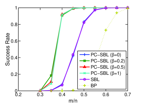
Figure 1: Success rates of the proposed algorithm vs. the ratio $m/n$ for different choices of $\beta$.

Next, we compare our proposed algorithm with some other recently developed algorithms for block-sparse signal recovery, namely, the expanded block sparse Bayesian learning method (EBSBL) [18], the Boltzman machine-based greedy pursuit algorithm (BM-MAP-OMP) [16], and the cluster-structured MCMC algorithm (CluSS-MCMC) [15]. The modified iterative reweighted $\ell_{1}$ method (denoted as MRL1) proposed in Section V is also examined in our simulations. Note that all these algorithms were developed without the knowledge of the block-sparse structure. The block sparse Bayesian learning method (denoted as BSBL) developed in [18] is included as well. Although the BSBL algorithm requires the knowledge of the block-sparse structure, it still provides decent performance if the presumed block size, denoted by $h$, is properly selected. Fig. 2 plots the success rates of respective algorithms as a function of the ratio $m/n$ and the sparsity level $K$, respectively. Simulation results show that our proposed algorithm achieves highest success rates among all algorithms and outperforms other methods by a considerable margin. We also noticed that the modified reweighted $\ell_{1}$ method (MRL1), although not as good as the proposed PD-SBL, still delivers acceptable performance which is comparable to the BSBL and better than the BM-MAP-OMP and the CluSS-MCMC.

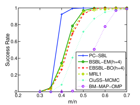
(a) Success rates vs. $m/n$, $n=100$, $K=25$, and $L=4$

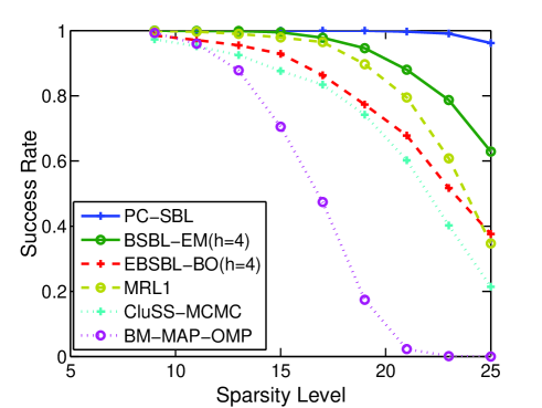
(b) Success rates vs. the sparsity level $K$, $m=40$, $n=100$, and $L=3$

Figure 2: Success rates of respective algorithms.

We now consider the noisy case where the measurements are contaminated by additive noise. The observation noise is assumed multivariate Gaussian with zero mean and covariance matrix $\sigma^{2}\boldsymbol{I}$. Also, in our simulations, the noise variance is assumed unknown (except for the BM-MAP-OMP). The NMSEs of respective algorithms as a function of the ratio $m/n$ and the sparsity level $K$ are plotted in Fig. 3, where the white Gaussian noise is added such that the signal-to-noise ratio (SNR), which is defined as $\text{SNR(dB)}\triangleq 20\log_{10}(\|\boldsymbol{Ax}\|_{2}/\|\boldsymbol{w}\|_{2})$, is equal to $15$dB for each iteration. We see that our proposed algorithm yields a lower estimation error than other methods in the presence of additive Gaussian noise.

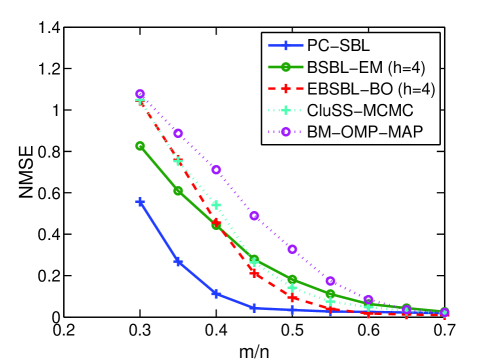
(a) Normalized MSEs vs. $m/n$, $n=100$, $K=25$, and $L=4$

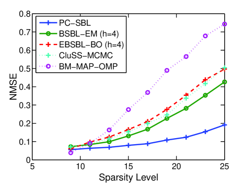
(b) Normalized MSEs vs. the sparsity level $K$, $m=40$, $n=100$, and $L=3$

Figure 3: Normalized MSEs of respective algorithms.

VI-B Real Data

In this subsection, we carry out experiments on real world images. As it is well-known, images have sparse (or approximately sparse) structures in certain over-complete basis, such as wavelet or discrete cosine transform (DCT) basis. Moreover, the sparse representations usually demonstrate clustered structures whose significant coefficients tend to be located together (see Fig. 6). Therefore images are suitable data sets for evaluating the effectiveness of a variety of block-sparse signal recovery algorithms. We consider two famous pictures ‘Lena’ and ‘Pirate’ in our simulations. In our experiments, the image is processed in a columnwise manner: we sample each column of the $128\times 128$ image using a randomly generated measurement matrix $\boldsymbol{A}\in\mathbb{R}^{m\times 128}$, recover each column from the $m$ measurements, and reconstruct the image based on the $128$ estimated columns. Fig. 4 and 5 show the original images ‘Lena’ and ‘Pirate’ and the reconstructed images using respective algorithms, where we set $m=64$ and $m=80$ respectively. We see that our proposed algorithm presents the finest image quality among all methods. The result, again, demonstrates its superiority over other existing methods. The reconstruction accuracy of respective algorithms can also be observed from the reconstructed wavelet coefficients. We provide the true wavelet coefficients of one randomly selected column from the image ‘Lena’, and the wavelet coefficients reconstructed by respective algorithms. Results are depicted in Fig. 6. It can be seen that our proposed algorithm provides reconstructed coefficients that are closest to the groundtruth.

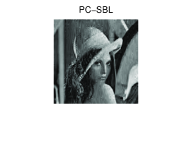
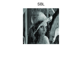
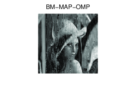
Figure 4: The original image ‘Lena’ and the reconstructed images using respective algorithms.

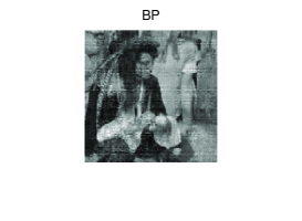
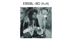
Figure 5: The original image ‘Pirate’ and the reconstructed images using respective algorithms.

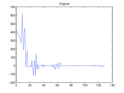
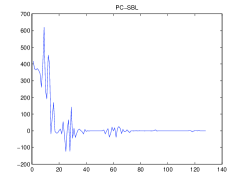
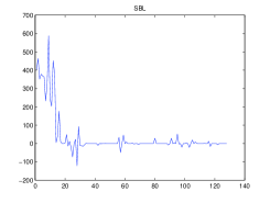
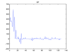
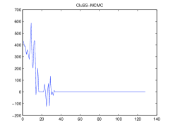
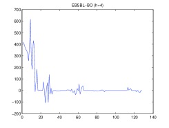
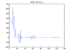
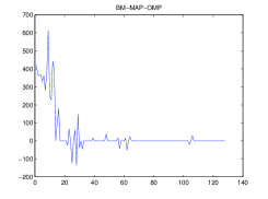
Figure 6: The true wavelet coefficients and the coefficients reconstructed by respective algorithms.

VII Conclusions

We developed a new Bayesian method for recovery of block-sparse signals whose block-sparse structures are entirely unknown. A pattern-coupled hierarchical Gaussian prior model was introduced to characterize both the sparseness of the coefficients and the statistical dependencies between neighboring coefficients of the signal. The prior model, similar to the conventional sparse Bayesian learning model, employs a set of hyperparameters to control the sparsity of the signal coefficients. Nevertheless, in our framework, the sparsity of each coefficient not only depends on its corresponding hyperparameter, but also depends on the neighboring hyperparameters. Such a prior has the potential to encourage clustered patterns and suppress isolated coefficients whose patterns are different from their respective neighbors. The hyperparameters, along with the sparse signal, can be estimated by maximizing their posterior probability via the expectation-maximization (EM) algorithm. Numerical results show that our proposed algorithm achieves a significant performance improvement as compared with the conventional sparse Bayesian learning method through exploiting the underlying block-sparse structure, even without knowing the exact locations and sizes of the non-zero blocks. It also demonstrates its superiority over other existing methods and provides state-of-the-art performance for block-sparse signal recovery.

References

- [1] S. S. Chen, D. L. Donoho, and M. A. Saunders, “Atomic decomposition by basis pursuit,” SIAM J. Sci. Comput., vol. 20, no. 1, pp. 33–61, 1998.
- [2] E. Candés and T. Tao, “Decoding by linear programming,” IEEE Trans. Information Theory, no. 12, pp. 4203–4215, Dec. 2005.
- [3] D. L. Donoho, “Compressive sensing,” IEEE Trans. Inform. Theory, vol. 52, pp. 1289–1306, 2006.
- [4] J. A. Tropp and A. C. Gilbert, “Signal recovery from random measurements via orthogonal matching pursuit,” IEEE Trans. Information Theory, vol. 53, no. 12, pp. 4655–4666, Dec. 2007.
- [5] M. J. Wainwright, “Information-theoretic limits on sparsity recovery in the high-dimensional and noisy setting,” IEEE Trans. Information Theory, vol. 55, no. 12, pp. 5728–5741, Dec. 2009.
- [6] W. Dai and O. Milenkovic, “Subspace pursuit for compressive sensing signal reconstruction,” IEEE Trans. Information Theory, no. 5, pp. 2230–2249, May 2009.
- [7] M. Mishali and Y. C. Eldar, “Blind multi-band signal reconstruction: compressed sensing for analog signals,” IEEE Trans. Signal Processing, vol. 57, no. 3, pp. 993–1009, Mar. 2009.
- [8] R. Gribonval and E. Bacry, “Harmonic decomposition of audio signals with matching pursuit,” IEEE Trans. Signal Processing, vol. 51, no. 1, pp. 101–111, Jan. 2003.
- [9] L. He and L. Carin, “Exploiting structure in wavelet-based Bayesian compressive sensing,” IEEE Trans. Signal Processing, vol. 57, no. 9, pp. 3488–3497, Sept. 2009.
- [10] Y. C. Eldar, P. Kuppinger, and H. Bölcskei, “Block-sparse signals: uncertainty relations and efficient recovery,” IEEE Trans. Information Theory, vol. 58, no. 6, pp. 3042–3054, June 2010.
- [11] Y. C. Eldar and M. Mishali, “Robust recovery of signals from a structured union of subspaces,” IEEE Trans. Information Theory, vol. 55, no. 11, pp. 5302–5316, Nov. 2009.
- [12] M. Yuan and Y. Lin, “Model selection and estimation in regression with grouped variables,” J. R. Statist. Soc. B, vol. 68, pp. 49–67, 2006.
- [13] J. Huang, T. Zhang, and D. Metaxas, “Learning with structured sparsity,” Journal of Machine Learning Research, vol. 12, pp. 3371–3412, 2011.
- [14] R. G. Baraniuk, V. Cevher, M. F. Duarte, and C. Hegde, “Model-based compressive sensing,” IEEE Trans. Information Theoy, vol. 56, no. 4, pp. 1982–2001, Apr. 2010.
- [15] L. Yu, H. Sun, J. P. Barbot, and G. Zheng, “Bayesian compressive sensing for cluster structured sparse signals,” Signal Processing, vol. 92, pp. 259–269, 2012.
- [16] T. Peleg, Y. C. Eldar, and M. Elad, “Exploiting statistical dependencies in sparse representations for signal recovery,” IEEE Trans. Signal Processing, vol. 60, no. 5, pp. 2286–2303, May 2012.
- [17] A. Drámeau, C. Herzet, and L. Daudet, “Boltzmann machine and mean-field approximation for structured sparse decompositions,” IEEE Trans. Signal Processing, vol. 60, no. 7, pp. 3425–3438, July 2012.
- [18] Z. Zhang and B. D. Rao, “Extension of SBL algorithms for the recovery of block sparse signals with intra-block correlation,” IEEE Trans. Signal Processing, vol. 61, no. 8, pp. 2009–2015, Apr. 2013.
- [19] M. Tipping, “Sparse Bayesian learning and the relevance vector machine,” Journal of Machine Learning Research, vol. 1, pp. 211–244, 2001.
- [20] S. Ji, Y. Xue, and L. Carin, “Bayesian compressive sensing,” IEEE Trans. Signal Processing, vol. 56, no. 6, pp. 2346–2356, June 2008.
- [21] J. Fang, S. Ji, Y. Xue, and L. Carin, “Multitask classification by learning the task relevance,” IEEE Signal Processing Letters, vol. 15, pp. 593–596, 2008.
- [22] D. P. Wipf, “Bayesian methods for finding sparse representations,” Ph.D. dissertation, University of California, San Diego, 2006.
- [23] D. P. Wipf and B. D. Rao, “An empirical Bayesian strategy for solving the simultaneous sparse approximation problem,” IEEE Trans. Signal Processing, vol. 55, no. 7, pp. 3704–3716, July 2007.
- [24] Z. Zhang and B. D. Rao, “Sparse signal recovery with temporally correlated source vectors using sparse Bayesian learning,” IEEE Journal of Selected Topics in Signal Processing, vol. 5, no. 5, pp. 912–926, Sept. 2011.
- [25] D. Wipf and S. Nagarajan, “Iterative reweighted and methods for finding sparse solutions,” IEEE Journals of Selected Topics in Signal Processing, vol. 4, no. 2, pp. 317–329, Apr. 2010.
- [26] E. Candès, M. B. Wakin, and S. P. Boyd, “Enhancing sparsity by reweighted minimization,” Journal of Fourier Analysis and Applications, vol. 14, pp. 877–905, Dec. 2008.