Abstract

In structured output learning, obtaining labeled data for real-world applications is usually costly, while unlabeled examples are available in abundance. Semi-supervised structured classification has been developed to handle large amounts of unlabeled structured data. In this work, we consider semi-supervised structural SVMs with domain constraints. The optimization problem, which in general is not convex, contains the loss terms associated with the labeled and unlabeled examples along with the domain constraints. We propose a simple optimization approach, which alternates between solving a supervised learning problem and a constraint matching problem. Solving the constraint matching problem is difficult for structured prediction, and we propose an efficient and effective hill-climbing method to solve it. The alternating optimization is carried out within a deterministic annealing framework, which helps in effective constraint matching, and avoiding local minima which are not very useful. The algorithm is simple to implement and achieves comparable generalization performance on benchmark datasets.

1 Introduction

Structured classification involves learning a classifier to predict objects like trees, graphs and image segments. Such objects are usually composed of several components with complex interactions, and are hence called “structured”. Typical structured classification techniques learn from a set of labeled training examples $\{({\bf{x}}_{i},{\bf{y}}_{i})\}_{i=1}^{l}$, where the instances ${\bf{x}}_{i}$ are from an input space $\mathscr{X}$ and the corresponding labels ${\bf{y}}_{i}$ belong to a structured output space $\mathscr{Y}$. Several efficient algorithms are available for fully supervised structured classification (see for e.g. Joachims et al. (2009); Balamurugan et al. (2011)). In many practical applications, however, obtaining the label of every training example is a tedious task and we are often left with only a very few labeled training examples.

When the training set contains only a few training examples with labels, and a large number of unlabeled examples, a common approach is to use semi-supervised learning methods (Chapelle et al., 2010). For a set of labeled training examples $\{({\bf{x}}_{i},{\bf{y}}_{i})\}_{i=1}^{l}$, ${\bf{x}}_{i}\in\mathscr{X}$, ${\bf{y}}_{i}\in\mathscr{Y}$ and a set of unlabeled examples $\{{\bf{x}}_{j}\}_{j=l+1}^{l+u}$, we consider the following semi-supervised learning problem:

$$\min_{{{\bf{w}}},{\bf{y}}_{j}^{*}\in\mathscr{Y}}\;\;\frac{1}{2}{\|{{\bf{w}}}\|^{2}}+\frac{C_{l}}{l}\sum_{i=1}^{l}L_{s}({\bf{x}}_{i},{\bf{y}}_{i};{\bf{w}})$$

$$+\frac{C_{u}}{u}\sum_{j=l+1}^{l+u}L_{u}({\bf{x}}_{j},{\bf{y}}_{j}^{*};{\bf{w}})$$

$${\rm s.t.}\;\;{\bf{y}}_{j}^{*}\in\mathscr{W},\;\forall\;j=l+1,\ldots,l+u,\;$$

$$\mathscr{W}=\bigcup_{k}\mathscr{W}_{k}$$

where $L_{s}(\cdot)$ and $L_{u}(\cdot)$ denote the loss functions corresponding to the labeled and unlabeled set of examples respectively. In addition to minimizing the loss functions, we also want to ensure that the predictions ${\bf{y}}_{j}^{*}$ over the unlabeled data satisfy a certain set of constraints: $\mathscr{W}=\bigcup_{k}\mathscr{W}_{k}$, determined using domain knowledge. Unlike binary or multi-class classification problem, the solution of (LABEL:general_semissvm) is hard due to each ${\bf{y}}_{j}^{*}$ having combinatorial possibilities. Further, the constraints play a key role in semi-supervised structured output learning, as demonstrated in (Chang et al., 2007; Dhillon et al., 2012). Chang et al. (2007) also provide a list of constraints (Table 1 in their paper), useful in sequence labeling. Each of these constraints can be expressed using a function, $\Phi:\mathscr{X}\times\mathscr{Y}\rightarrow T$, where $T=\{0,1\}$ for hard constraint or $T=\mathbb{R}$ for soft constraints. For example, the constraint that “a citation can only start with author” is a hard constraint and the violation of this constraint can be denoted as $\Phi_{1}({\bf{x}}_{j},{\bf{y}}_{j}^{*})=1$. On the other hand. the constraint that “each output at has at least one author” can be expressed as $\Phi_{2}({\bf{x}}_{j},{\bf{y}}_{j}^{*})\geq 1$. Violation of constraints can be penalized by using an appropriate constraint loss function $\mathscr{C}(\Phi_{k}({\bf{x}}_{j},{\bf{y}}_{j}^{*})-c)$ in the objective function. The domain constraints $\Phi(\mathscr{X},\mathscr{Y})$ can be further divided into two broad categories, namely the instance level constraints, which are imposed over individual training examples, and the corpus level constraints, imposed over the entire corpus.

By extending the binary transductive SVM algorithm proposed in (Joachims, 1999) and constraining the relative frequencies of the output symbols,  Zien et al. (2007) proposed to solve the transductive SVM problem for structured outputs. Small improvement in performance over purely supervised learning was observed, possibly because of lack of domain dependent prior knowledge. Chang et al. (2007) proposed a constraint-driven learning algorithm (CODL) by incorporating domain knowledge in the constraints and using a perceptron style learning algorithm. This approach resulted in high performance learning using significantly less training data. Bellare et al. (2009) proposed an alternating projection method to optimize an objective function, which used auxiliary expectation constraints.  Ganchev et al. (2010) proposed a posterior regularization (PR) method to optimize a similar objective function. Yu (2012) considered transductive structural SVMs and used a convex-concave procedure to solve the resultant non-convex problem.

Closely related to our proposed method is the Deterministic Annealing for Structured Output (DASO) approach proposed in (Dhillon et al., 2012). It deals with the combinatorial nature of the label space by using relaxed labeling on unlabeled data. It was found to perform better than the approaches like CODL and PR. However, DASO has not been explored for large-margin methods. Moreover, dealing with combinatorial label space is not straightforward for large-margin methods and the relaxation idea proposed in (Dhillon et al., 2012) cannot be easily extended to handle large-margin formulation. This paper has the following important contributions in the context of semi-supervised large-margin structured output learning.

Contributions: In this paper, we propose an efficient algorithm to solve semi-supervised structured output learning problem (LABEL:general_semissvm) in the large-margin setting. Alternating optimization steps (fix ${\bf{y}}_{j}^{*}$ and solve for ${\bf{w}}$, and then fix ${\bf{w}}$ and solve for ${\bf{y}}_{j}^{*}$) are used to solve the problem. While solving (LABEL:general_semissvm) for ${\bf{w}}$ can be done easily using any known algorithm, finding optimal ${\bf{y}}_{j}^{*}$ for a fixed ${\bf{w}}$ requires combinatorial search. We propose an efficient and effective hill-climbing method to solve the combinatorial label switching problem. Deterministic Annealing is used in conjunction with alternating optimization to avoid poor local minima. Numerical experiments on two real-world datasets demonstrate that the proposed algorithm gives comparable or better results with those reported in (Dhillon et al., 2012) and (Yu, 2012), thereby making the proposed algorithm a useful alternative for semi-supervised structured output learning.

The paper is organized as follows. The next section discusses related work on semi-supervised learning techniques for structured output learning. Section 3 explains the deterministic annealing solution framework for semi-supervised training of structural SVMs with domain constraints. The label-switching procedure is elaborated in section 4. Empirical results on two benchmark datasets are presented in section 5. Section 6 concludes the paper.

2 Related Work

A related work to our approach is the transductive SVM (TSVM) for multi-class and hierarchical classification by (Keerthi et al., 2012), where the idea of TSVMs in (Joachims, 1999) was extended to multi-class problems. The main challenge for multi-class problems was in designing an efficient procedure to handle the combinatorial optimization involving the labels $y_{j}^{*}$ for unlabeled examples. Note that for multi-class problems, $y_{j}^{*}\in\{1,2,\ldots,k\}$ for some $k\geq 3$. Keerthi et al. (2012) showed that the combinatorial optimization for multi-class label switching results in an integer program, and proposed a transportation simplex method to solve it approximately. However, the transportation simplex method turned out to be in-efficient and an efficient label-switching procedure was given in (Keerthi et al., 2012). A deterministic annealing method and domain constraints in the form of class-ratios were also used in the training. We note however that a straightforward extension of TSVM to structured output learning is hindered by the complexity of solving the associated label switching problem. Extending the label switching procedure to structured outputs is much more challenging, due to their complex structure and the large cardinality of the output space.

Semi-supervised structural SVMs considered in  (Zien et al., 2007) avoid the combinatorial optimization of the structured output labels, and instead consider a working set of labels. We also note that the combinatorial optimization of the label space is avoided in the recent work on transductive structural SVMs by (Yu, 2012); instead, a working set of cutting planes is maintained. The other related work DASO (Dhillon et al., 2012) too does not consider the combinatorial problem of the label space directly; rather, it solves a problem of the following form:

$$\min_{{\bf{w}},a}R({\bf{w}})+{\mathbb{E}}_{a}L(\mathscr{Y};\mathscr{X},{\bf{w}})+\mathscr{C}({\mathbb{E}}_{a}[\Phi(\mathscr{X},\mathscr{Y})]-c)$$ (2)

where $a$ denotes a distribution $a(\mathscr{Y})$ over the label space and $L(\mathscr{Y};\mathscr{X},{\bf{w}})$ is considered to be the log-linear loss. Including the distribution $a(\mathscr{Y})$ avoids dealing with the original label space $\mathscr{Y}$ and side-steps the combinatorial problem over label space. Hence, to the best of our knowledge, no prior work exists, which tackles directly the combinatorial optimization problem involving structured outputs.

3 Semi-supervised learning of structural SVMs

We consider the sequence labeling problem as a running example throughout this paper. The sequence labeling problem is a well-known structured classification problem, where a sequence of entities ${\bf{x}}=(x^{1},x^{2},\ldots,x^{M})$ is labeled using corresponding sequence of labels ${\bf{y}}=(y^{1},y^{2},\ldots,y^{M})$. The labels $\{y^{j}\}_{j=1}^{M}$ are assumed to be from a fixed alphabet $\Omega$ of size $|\Omega|$. Consider a structured input-output space pair $(\mathscr{X},\mathscr{Y})$. Given a training set of labeled examples $\{({\bf{x}}_{i},{\bf{y}}_{i})\}_{i=1}^{l}\;\in(\mathscr{X}\times\mathscr{Y})$, structural SVMs learn a parametrized classification rule $h:\mathscr{X}\rightarrow\mathscr{Y}$ of the form $h({\bf{x}};{\bf{w}})=\arg\max_{{\bf{y}}}{\bf{w}}^{T}f({\bf{x}},{\bf{y}})$ by solving the following convex optimization problem:

$$\min_{{{\bf{w}}},\xi_{i}\geq 0}\;\;\;\;\frac{1}{2}{\|{{\bf{w}}}\|^{2}}+C\sum_{i=1}^{l}\xi_{i}({\bf{x}}_{i},{\bf{y}}_{i},{\bf{w}})$$

$${\rm s.t.}\;\;\;\;\xi_{i}\geq\delta_{i}({{\bf{y}}}_{i},{{\bf{y}}})-{{\bf{w}}}^{T}{\Delta f_{i}({{\bf{y}}}_{i},{{\bf{y}}})},$$

$$\forall\;i=1,\ldots,l,\;\forall\;{\bf{y}}\in\mathscr{Y}.$$

An input ${\bf{x}}_{i}$ is associated with the output ${\bf{y}}_{i}$ of the same length and this association is captured using the feature vector $f({\bf{x}}_{i},{\bf{y}}_{i})$. The notation $\Delta f_{i}({{\bf{y}}}_{i},{{\bf{y}}})$ in (LABEL:ssvm_primal) is given by $f({\bf{x}}_{i},{\bf{y}}_{i})-f({\bf{x}}_{i},{\bf{y}})$, the difference between the feature vectors corresponding to ${\bf{y}}_{i}$ and ${\bf{y}}$, respectively. The notation $\delta_{i}({{\bf{y}}}_{i},{{\bf{y}}})=\delta({\bf{x}}_{i},{\bf{y}}_{i},{\bf{y}})$ is a suitable loss term. For sequence labeling applications, $\delta_{i}({{\bf{y}}}_{i},{{\bf{y}}})$ can be chosen to be the Hamming loss function. $C>0$ is a regularization constant.

With the availability of a set of unlabeled examples $\{{\bf{x}}_{j}\}_{j=l+1}^{l+u}\in\mathscr{X}$, the semi-supervised learning problem for structural SVMs is given by:

$$\min_{{{\bf{w}}},\xi_{i}\geq 0,\xi_{j}^{*}\geq 0}\;\;\;\;\frac{1}{2}{\|{{\bf{w}}}\|^{2}}+\frac{C_{l}}{l}\sum_{i=1}^{l}\xi_{i}({\bf{x}}_{i},{\bf{y}}_{i},{\bf{w}})$$

$$+{\frac{C_{u}}{u}}\sum_{j=l+1}^{l+u}\xi_{j}^{*}({\bf{x}}_{j},{\bf{y}}_{j}^{*},{\bf{w}})$$

$${\rm s.t.}\;\;\;\;\xi_{i}\geq\delta_{i}({{\bf{y}}}_{i},{{\bf{y}}})-{{\bf{w}}}^{T}{\Delta f_{i}({{\bf{y}}}_{i},{{\bf{y}}})}\;$$

$$\forall\;i=1,\cdots,l,\;\forall\;{\bf{y}}\in\mathscr{Y},$$

$$\xi_{j}^{*}=\min_{{\bf{y}}_{j}^{*}\in\mathscr{Y}}\max_{{\bf{y}}\in\mathscr{Y}}\;\delta_{j}({{\bf{y}}_{j}^{*}},{{\bf{y}}})-{{\bf{w}}}^{T}{\Delta f_{j}({{\bf{y}}_{j}^{*}},{{\bf{y}}})}$$

$$\;\forall\;j=l+1,\cdots,l+u.$$

The problem (LABEL:zien_s3svm_primal) was considered in (Zien et al., 2007), where a working-set idea was proposed to handle the optimization with respect to $\xi_{j}^{*}$. However, domain knowledge was not incorporated into the problem (LABEL:zien_s3svm_primal). We consider the following non-convex problem for semi-supervised learning of structural SVMs, which contain the domain constraints:

$$\min_{{{\bf{w}}},\xi_{i}\geq 0,\xi_{j}^{*}\geq 0}\;\;\;\;\frac{1}{2}{\|{{\bf{w}}}\|^{2}}+\frac{C_{l}}{l}\sum_{i=1}^{l}\xi_{i}({\bf{x}}_{i},{\bf{y}}_{i},{\bf{w}})+$$

$${\frac{C_{u}}{u}}\sum_{j=l+1}^{l+u}\xi_{j}^{*}({\bf{x}}_{j},{\bf{y}}_{j}^{*},{\bf{w}})+\mathscr{C}(\Phi(\mathscr{X},\mathscr{Y})-c)$$

$${\rm s.t.}\;\;\;\;\xi_{i}\geq\delta_{i}({{\bf{y}}}_{i},{{\bf{y}}})-{{\bf{w}}}^{T}{\Delta f_{i}({{\bf{y}}}_{i},{{\bf{y}}})}$$

$$\forall\;i=1,\cdots,l,\;\forall\;{\bf{y}}\in\mathscr{Y},$$

$$\xi_{j}^{*}=\min_{{\bf{y}}_{j}^{*}\in\mathscr{Y}}\max_{{\bf{y}}\in\mathscr{Y}}\;\delta_{j}({{\bf{y}}_{j}^{*}},{{\bf{y}}})-{{\bf{w}}}^{T}{\Delta f_{j}({{\bf{y}}_{j}^{*}},{{\bf{y}}})}$$

$$\forall\;j=l+1,\cdots,l+u.$$

Note that the problem (LABEL:s3svm_primal) is an extension of the semi-supervised learning problems associated with binary (Joachims, 1999) and multi-class (Keerthi et al., 2012) outputs. $C_{u}$, the regularization constant associated with the unlabeled examples, is chosen using an annealing procedure, which gradually increases the influence of unlabeled examples in the training (Dhillon et al., 2012; Keerthi et al., 2012).

The objective function in (LABEL:s3svm_primal) is non-convex and hence we resort to an alternating optimization approach, which is an extension of the procedure given in (Keerthi et al., 2012) for semi-supervised multi-class and hierarchical classification. We note however that this extension is not easy. This will become clear when we describe the constraint matching problem.

A supervised learning problem is solved to obtain an initial model ${\bf{w}}$ before the alternating optimization is performed. This supervised learning is done only with the labeled examples, by solving (LABEL:ssvm_primal). With an initial estimate of ${\bf{w}}$ available in hand, the alternating optimization procedure starts by solving the constraint matching problem with respect to $\xi_{j}^{*}$:

$$\min_{\xi_{j}^{*}\geq 0}\;\;\;\;{\frac{C_{u}}{u}}\sum_{j=l+1}^{l+u}\xi_{j}^{*}({\bf{x}}_{j},{\bf{y}}_{j}^{*},{\bf{w}})+\mathscr{C}(\Phi(\mathscr{X},\mathscr{Y})-c)$$

$${\rm s.t.}\;\;\;\;\xi_{j}^{*}=\min_{{\bf{y}}_{j}^{*}\in\mathscr{Y}}\max_{{\bf{y}}\in\mathscr{Y}}\;\delta_{j}({{\bf{y}}_{j}^{*}},{{\bf{y}}})-{{\bf{w}}}^{T}{\Delta f_{j}({{\bf{y}}_{j}^{*}},{{\bf{y}}})}$$

$$\forall\;j=l+1,\cdots,l+u.$$

Note that the objective function in the problem (LABEL:constraintmatchprob) is linear in $\xi_{j}^{*}$. However, it also contains the penalty term on domain constraints $\mathscr{C}(\Phi(\mathscr{X},\mathscr{Y})-c)$. The constraints involving $\xi_{j}^{*}$ are not simple, and finding the quantity

$$\xi_{j}^{*}=\min_{{\bf{y}}_{j}^{*}\in\mathscr{Y}}\max_{{\bf{y}}\in\mathscr{Y}}\;\delta_{j}({{\bf{y}}_{j}^{*}},{{\bf{y}}})-{{\bf{w}}}^{T}{\Delta f_{j}({{\bf{y}}_{j}^{*}},{{\bf{y}}})}$$ (7)

becomes difficult when the domain constraints $\Phi(\mathscr{X},\mathscr{Y})$ are also considered. Hence an efficient procedure needs to be designed to solve (LABEL:constraintmatchprob). In the next section, we propose an efficient label-switching procedure to find a set of candidate outputs $\{{\bf{y}}_{j}^{*}\}_{j=l+1}^{l+u}$ for the constraint matching problem (LABEL:constraintmatchprob). Once we find $\{{\bf{y}}_{j}^{*}\}_{j=l+1}^{l+u}$, the alternating optimization moves on to solve (LABEL:s3svm_primal) for ${\bf{w}}$, with $\{{\bf{y}}_{j}^{*}\}_{j=l+1}^{l+u}$ remaining fixed. After solving (LABEL:s3svm_primal), the alternating optimization solves (LABEL:constraintmatchprob) again, for a fixed ${\bf{w}}$. This procedure is repeated until some suitable stopping criterion is satisfied.

The alternating optimization procedure described above, is carried out within a deterministic annealing framework. The regularization constant $C_{u}$ associated with the unlabeled examples is slowly varied in the annealing step. Maintaining a fixed value of $C_{u}$ is often not useful, and using cross-validation to find a suitable value for $C_{u}$ is also not possible. Hence, the deterministic annealing framework provides a useful way to get a reasonable value of $C_{u}$. In our experiments, $C_{u}$ was varied over the range $\{10^{-4},3\times 10^{-4},10^{-3},3\times 10^{-3},\ldots,1\}$. We describe the alternating optimization along with the deterministic annealing procedure in Algorithm 1.

Algorithm 1 A Deterministic Annealing -Alternating Optimization algorithm to solve (LABEL:s3svm_primal)

1:  Input labeled examples $\{({{\bf{x}}}_{i},{{\bf{y}}}_{i})\}^{n}_{i=1}$ and unlabeled examples $\{{{\bf{x}}}_{j}\}^{l+u}_{j=l+1}$.

2:  Input $C_{l}$, the regularization constant and $\Omega$, the alphabet for labels.

3:  Set maxiter = 1000.

4:  Obtain ${\bf{w}}$ by solving the supervised learning problem in (LABEL:ssvm_primal).

5:  for $C_{u}=10^{-4},3\times 10^{-4},10^{-3},3\times 10^{-3},\ldots,1$ do

6:     iter:=1

7:     repeat

8:        Obtain ${\{{\bf{y}}_{j}^{*}\}}_{j=l+1}^{l+u}$ for unlabeled examples by solving the constraint matching problem (LABEL:constraintmatchprob) using Algorithm 2.

9:        Obtain ${\bf{w}}$ by solving (LABEL:s3svm_primal) with ${\bf{y}}_{j}^{*}$ as the actual labels for ${\bf{x}}_{j},\;j=l+1,\ldots,l+u$.

10:        iter:=iter+1

11:     until the labeling ${\bf{y}}_{j}^{*}$ does not change for unlabeled examples or iter$>$maxiter

12:  end for

4 Label switching algorithm to solve (LABEL:constraintmatchprob)

In this section, we describe an efficient approach to solve the constraint matching problem given by (LABEL:constraintmatchprob). We note that finding $\xi_{j}^{*}$ using the relation (7) involves solving a complex combinatorial optimization problem. Hence, a useful heuristic is to fix a ${\bf{y}}_{j}^{*}\in\mathscr{Y}$, and find a corresponding ${\bf{y}}\in\mathscr{Y}$, such that the quantity $\delta_{j}({{\bf{y}}_{j}^{*}},{{\bf{y}}})-{{\bf{w}}}^{T}{\Delta f_{j}({{\bf{y}}_{j}^{*}},{{\bf{y}}})}$ is maximized with respect to ${\bf{y}}_{j}^{*}$. An important step is to find a good candidate for ${\bf{y}}_{j}^{*}$, such that the constraint violation $\mathscr{C}(\Phi(\mathscr{X},\mathscr{Y})-c)$ is minimized. We propose to choose ${\bf{y}}_{j}^{*}$ by an iterative label-switching procedure, which we describe in detail below.

Since the constraint matching problem (Step 8 in Algorithm 1) always follows a supervised learning step, we have an estimate of ${\bf{w}}$, before we solve the constraint matching problem. With this current estimate of ${\bf{w}}$, we can find an initial candidate ${\bf{y}}_{j}^{*}$ for an unlabeled example ${\bf{x}}_{j}$ as:

$${\bf{y}}_{j}^{*}=\arg\max_{{\bf{y}}\in\mathscr{Y}}{{\bf{w}}}^{T}f({\bf{x}}_{j},{\bf{y}}).$$ (8)

The availability of candidate ${\bf{y}}_{j}^{*}$ for all unlabeled examples $j=l+1,\ldots,l+u$, makes it possible to compute the objective term in (LABEL:constraintmatchprob), where $\xi_{j}^{*}$ for the fixed ${\bf{y}}_{j}^{*}$ is obtained using

$$\xi_{j}^{*}=\arg\max_{{\bf{y}}\in\mathscr{Y}}\delta_{j}({{\bf{y}}_{j}^{*}},{{\bf{y}}})-{{\bf{w}}}^{T}{\Delta f_{j}({{\bf{y}}_{j}^{*}},{{\bf{y}}})}.$$ (9)

Let us denote the objective value in (LABEL:constraintmatchprob) by ${\mathscr{O}}^{*}$ and let the length of the sequence ${\bf{x}}_{j}=(x_{j}^{1},x_{j}^{2},\ldots,x_{j}^{M})$ be $M$. We now iteratively pass over the components $x_{j}^{m}$, $\forall\;m=1,2,\ldots,M$, and switch the label components $y_{j}^{m}$. Recall that the label components $y_{j}^{m}$ are from a finite alphabet $\Omega$ of size $|\Omega|$. The switching is done randomly by replacing the label component $y_{j}^{m}$ with a new label $y^{r}\in\Omega$. With this replacement, we compute the constraint violation $\mathscr{C}(\Phi(\mathscr{X},\mathscr{Y})-c)$ and the slack term $\xi_{j}^{*}$. If the replacement causes a decrease in the objective value ${\mathscr{O}}^{*}$, then we keep the new label $y^{r}$ for the $m$-th component and move on to the next component. If there is no decrease in the objective value, we ignore the replacement and keep the original label. Note that the constraint matching is handled for each replacement as follows. Whenever a new label is considered for the $m$-th component, instance level constraint violation can be checked with the new label in a straightforward way. Any corpus level constraint violation is usually decomposable over the instances and can also be handled in a simple way. Hence the constraint violation term $\mathscr{C}(\Phi(\mathscr{X},\mathscr{Y})-c)$ can be computed for each replacement. This ensures that by switching the labels, we do not violate the constraints too much. Apart from choosing the label $y^{r}$ for the $m$-th component randomly, the component $m$ itself was randomly selected in our implementation. The switching procedure is stopped when there is no sufficient decrease in the objective value term in (LABEL:constraintmatchprob) or when a prescribed upper limit on the number of label switches is exceeded. The overall procedure is illustrated in Algorithm 2.

Algorithm 2 A label switching algorithm to solve constraint matching problem (LABEL:constraintmatchprob)

1:  Input unlabeled example ${\bf{x}}_{j}$

2:  Input ${\bf{w}}$, $C_{u}$

3:  Set maxswitches = 1000, numswitches=0

4:  for $j=l+1,\ldots,l+u$ do

5:     Find initial candidate ${\bf{y}}_{j}^{*}$ by (8)

6:     Compute slack $\xi_{j}^{*}$ and constraint violation $\mathscr{C}(\Phi(\mathscr{X},\mathscr{Y})-c)$.

7:  end for

8:  Calculate objective value

$${\mathscr{O}}^{*}={\frac{C_{u}}{u}}\sum_{j=l+1}^{l+u}\xi_{j}^{*}({\bf{x}}_{j},{\bf{y}}_{j}^{*},{\bf{w}})+\mathscr{C}(\Phi(\mathscr{X},\mathscr{Y})-c).$$

9:  for $j=l+1,\ldots,l+u$ do

10:     $\hat{\bf{y}}_{j}={\bf{y}}_{j}^{*}$, $M=length(\hat{\bf{y}})$, $mincost={\mathscr{O}}^{*}$

11:     for $m=1,\dots,M$ do

12:        $y^{m}$$=$$m^{th}$ label component of $\hat{\bf{y}}$, $mincostlabel$$=$$y^{m}$

13:        for $y^{r}\in\Omega$ and $y^{r}\neq y^{m}$ do

14:           Replace $y^{m}$ with $y^{r}$.

15:           Compute $\mathscr{C}(\phi(\mathscr{X},\mathscr{Y})$$-$$c)$, the constraint violation.

16:           Find violator for ${\hat{\bf{y}}}_{j}$ as

$${\bar{{\bf{y}}}}=\arg\max_{{\bf{y}}}\{{\bf{w}}^{T}f({\bf{x}}_{j},{\bf{y}})+\delta_{j}(\hat{\bf{y}}_{j},{\bf{y}})\}.$$

17:           Compute slack

$$\xi(\hat{\bf{y}}_{j})=\max(0,{\bf{w}}^{T}\Delta f_{j}(\hat{\bf{y}}_{j},\bar{{\bf{y}}})+\delta_{j}(\hat{\bf{y}}_{j},\bar{{\bf{y}}})).$$

18:           Compute objective value of (LABEL:constraintmatchprob) as $\hat{\mathscr{O}}$.

19:           if $\hat{\mathscr{O}}$$<$$mincost$ then

20:              $mincost$ = $\hat{\mathscr{O}}$,   $mincostlabel=y^{r}$

21:           end if

22:        end for

23:        Replace $m^{th}$ label of ${\bf{y}}_{j}^{*}$ with $mincostlabel$

24:        numswitches = numswitches + 1

25:        if numswitches $>$ maxswitches then

26:           Goto Step 30

27:        end if

28:     end for

29:  end for

30:  Output ${\{{\bf{y}}_{j}^{*}\}}_{j=l+1}^{l+u}$.

5 Experiments and Results

We performed experiments with the proposed semi-supervised structured classification algorithm on two benchmark sequence labeling datasets; the citations and apartment advertisements. These datasets and were originally introduced in (Grenager et al., 2005) and contain manually-labeled training and test examples. The datasets also contain a set of unlabeled examples, which is proportionally large when compared to the training set. The annealing schedule was performed as follows: the annealing temperature was started at $10^{-4}$ and increased in small steps and stopped at $1$. The evaluation is done in terms of labeling accuracy on the test data obtained by the model at the end of training. We used the sequential dual method (SDM) (Balamurugan et al., 2011) for supervised learning (Step 4 in Algorithm 1) and compared the following methods for our experiments:

• Semi-supervised structural SVMs proposed in this paper (referred to as SSVM-SDM)

• Constraint-driven Learning (Chang et al., 2007) (referred to as CODL)

• Deterministic Annealing for semi-supervised structured classification (Dhillon et al., 2012) (referred to as DASO)

• Posterior-Regularization (Ganchev et al., 2010) (referred to as PR)

• Transductive structural SVMs (Yu, 2012) (referred to as Trans-SSVM)

The apartments dataset contains 300 sequences from craigslist.org. These sequences are labeled using a set of 12 labels like features, rent, contact, photos, size and restriction. The average sequence length is 119. The citations dataset contains 500 sequences, which are citations of computer science papers. The labeling is done from a set of 13 labels like author, title, publisher, pages, and journal. The average sequence length for citation dataset is 35.

The description and split sizes of the datasets are given in Table 1. The partitions of citation data was taken to be the same as considered in Dhillon et al. (2012). For apartments dataset, we considered datasets of 5, 20 and 100 labeled examples. We generated 5 random partitions for each case and provide the averaged results over these partitions.

Table 1: Dataset Characteristics

Dataset	$n_{labeled}$	$n_{dev}$	$n_{unlabeled}$	$n_{test}$
citation	5; 20; 300	100	1000	100
apartments	5; 20; 100	100	1000	100

Table 2: Comparison of average test accuracy(%) obtained from SSVM-SDM with results in (Dhillon et al., 2012) (denoted by ^$) and (Yu, 2012) (denoted by ^∗) for Citation Dataset. (I) denotes inductive setting, in which test examples were not used as unlabeled examples for training. (no I) denotes the setting where test examples were used as unlabeled examples for training. ^∗Note that different set of features were considered in (Yu, 2012).

$n_{labeled}$	Baseline CRF$	Baseline SDM	DASO$	SSVM-SDM	PR$	CODL$	Trans-SSVM∗
			(I)	(I)	(I)	(I)	(no I)
5	63.1	66.82	75.2	74.74	62.7	71	72.8
20	79.1	78.25	84.9	86.2	76	79.4	81.4
300	89.9	91.54	91.1	92.92	87.29	88.8	92.8

Table 3: Comparison of average test accuracy(%) obtained from SSVM-SDM with results in (Dhillon et al., 2012) (denoted by ^$) and (Yu, 2012) (denoted by ^∗) for Apartments Dataset. (I) denotes inductive setting, in which test examples were not used as unlabeled examples for training. (no I) denotes the setting where test examples were used as unlabeled examples for training. ^∗Note that different set of features and split sizes were considered in (Yu, 2012).

$n_{labeled}$	Baseline CRF$	Baseline SDM	DASO$	SSVM-SDM	PR$	CODL$	Trans-SSVM∗
			(I)	(I)	(I)	(I)	(no I)
5	65.1	64.06	67.9	68.28	66.5	66	Not Available
20	72.7	73.63	76.2	76.37	74.9	74.6	Not Available
100	76.4	79.95	80	81.93	79	78.6	78.6

5.1 Description of the constraints

We describe the instance level and corpus level constraints considered for citations data. A similar description holds for those of apartment dataset. We used the same set of constraints given in (Chang et al., 2007; Dhillon et al., 2012). The constraints considered are of the form $\Phi(\mathscr{X},\mathscr{Y})-c$, which are further sub-divided into instance level constraints of the form

$$\Phi_{I}(\mathscr{X},\mathscr{Y})=\phi_{I}({\bf{x}}_{j},{\bf{y}}_{j}^{*}),\;\;j=l+1,\cdots,l+u$$ (10)

and the corpus level constraints of the form $\Phi_{D}(\mathscr{X},\mathscr{Y})-c_{D}$ where

$$\Phi_{D}(\mathscr{X},\mathscr{Y})=\sum_{j=l+1}^{l+u}\phi_{D}({\bf{x}}_{j},{\bf{y}}_{j}^{*}).$$ (11)

We consider the following examples for instance level domain constraints.

1. AUTHOR label list can only appear at most once in each citation sequence : For this instance level constraint, we could consider

$$\phi_{I_{1}}({\bf{x}}_{j},{\bf{y}}_{j}^{*})=\text{Number of $AUTHOR$ label lists in ${\bf{y}}_{j}^{*}$}$$

and the corresponding $c_{I}$ to be 1. Hence the instance level domain constraint is of the form $\phi_{I_{1}}({\bf{x}}_{j},{\bf{y}}_{j}^{*})\leq 1$. The penalty function could then be defined as

$$\mathscr{C}(\phi_{I_{1}}({\bf{x}}_{j},{\bf{y}}_{j}^{*})-1)=r|\phi_{I_{1}}({\bf{x}}_{j},{\bf{y}}_{j}^{*})-1|^{2}$$

where $r$ is a suitable penalty scaling factor. We used $r=1000$ for our experiments.

2. The word CA is LOCATION : For this instance level constraint, we could consider

$$\phi_{I_{2}}({\bf{x}}_{j},{\bf{y}}_{j}^{*})=\mathscr{I}\text{(Label for word CA in ${\bf{y}}_{j}^{*}$}$$

== LOCATION)

where $\mathscr{I}(z)$ is the indicator function which is 1 if $z$ is true and $0$ otherwise. The corresponding $c_{I}$ for this constraint is set to 1. Hence the instance level domain constraint is of the form $\phi_{I_{2}}({\bf{x}}_{j},{\bf{y}}_{j}^{*})=1$. The penalty function could then be defined as

$$\mathscr{C}(\phi_{I_{2}}({\bf{x}}_{j},{\bf{y}}_{j}^{*})-1)=r$$

3. Each label must be a consecutive list of words and can occur atmost only once : For this instance level constraint, we could consider

$$\phi_{I_{3}}({\bf{x}}_{j},{\bf{y}}_{j}^{*})=\text{Number of labels which appear}$$

more than once as disjoint lists in $${\bf{y}}_{j}^{*}$$

The corresponding $c_{I}$ for this constraint is set to 0. Hence the instance level domain constraint is of the form $\phi_{I_{3}}({\bf{x}}_{j},{\bf{y}}_{j}^{*})=0$. The penalty function could then be defined as

$$\mathscr{C}(\phi_{I_{3}}({\bf{x}}_{j},{\bf{y}}_{j}^{*}))=r|\phi_{I_{3}}({\bf{x}}_{j},{\bf{y}}_{j}^{*})|^{2}$$

Next, we consider some corpus level constraints.

1. 30% of tokens should be labeled AUTHOR : For this corpus level constraint, we could consider

$$\Phi_{D_{1}}(\mathscr{X},\mathscr{Y})=\text{Percentage of $AUTHOR$ labels in $\mathscr{Y}$}$$

and the corresponding $c_{I}$ to be 30. Hence the corpus level domain constraint is of the form $\phi_{D_{1}}(\mathscr{X},\mathscr{Y})=30$. The penalty function could then be defined as

$$\mathscr{C}(\phi_{D_{1}}(\mathscr{X},\mathscr{Y})-30)=r|\phi_{D_{1}}(\mathscr{X},\mathscr{Y})-30|^{2}$$

2. Fraction of label transitions that occur on non-punctuation characters is 0.01 : For this corpus level constraint, we could consider

$$\phi_{D_{2}}(\mathscr{X},\mathscr{Y})=\text{Fraction of label transitions}$$

that occur on non-punctuation characters

The corresponding $c_{I}$ for this constraint is set to 0.01. Hence the corpus level domain constraint is of the form $\phi_{D_{2}}(\mathscr{X},\mathscr{Y})=0.01$. The penalty function could then be defined as

$$\mathscr{C}(\phi_{D_{2}}(\mathscr{X},\mathscr{Y})-0.01)=r|\phi_{D_{2}}(\mathscr{X},\mathscr{Y})-0.01|.$$

5.2 Experiments on the citation data

We considered the citation dataset with 5, 20 and 300 labeled examples, along with 1000 unlabeled examples and measured the performance on a test set of 100 examples. The parameter $C_{l}$ was tuned using a development dataset of 100 examples. The average performance on the test set was computed by training on five different partitions for each case of 5, 20 and 300 labeled examples. The average test set accuracy comparison is presented in Table 2.

The results for CODL, DASO and PR are quoted from the Inductive setting in (Dhillon et al., 2012), as the same set of features and constraints in (Dhillon et al., 2012) are used for our experiments and test examples were not considered for our training. With respect to Trans-SSVMs, we quote the results for non-Inductive setting from (Yu, 2012), in which constraints were not used for prediction. However, we have the following important differences with Trans-SSVM in terms of the features and constraints. The feature set used for Trans-SSVM is not the same as that used for our experiments. Test examples were used for training Trans-SSVMs, which is not done for SSVM-SDM. Hence, the comparison results in Table 2 for Trans-SSVM are only indicative. From the results in Table 2, we see that, for citations dataset with 5 labeled examples, the performance of SSVM-SDM is slightly worse when compared to that obtained for DASO. However, for other datasets, SSVM-SDM achieves a comparable performance.

We present the plots on test accuracy and primal objective value for the partitions containing 5, 20 and 300 examples, in Figure 1. These plots indicate that as the annealing temperature increases, the generalization performance increases initially and then continues to drop. This drop in generalization performance might possibly be the result of over-fitting caused by an inappropriate weight $C_{u}$ for unlabeled examples. Similar observation has been made in other semi-supervised structured output learning work using deterministic annealing (Chang et al., 2013). These observations suggest that finding a suitable stopping criterion for semi-supervised structured output learning in the deterministic annealing framework requires further study. For our comparison results, we considered the maximum test accuracy obtained from the experiments. This is indicated by a square marker in the test accuracy plots in Figure 1.

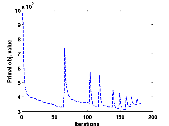
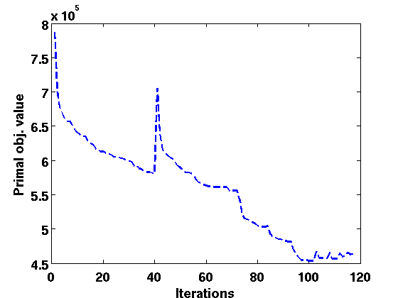
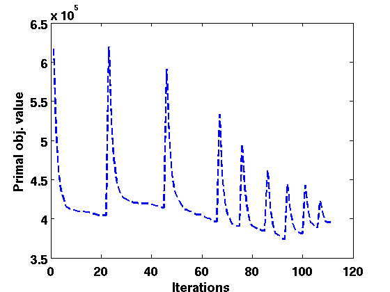
Figure 1: Primal objective value and Test accuracy behaviour for a partition of citations dataset. The rows correspond to 5, 20 and 300 labeled examples in that order. The square marker in the test accuracy plots denotes the best generalization performance.

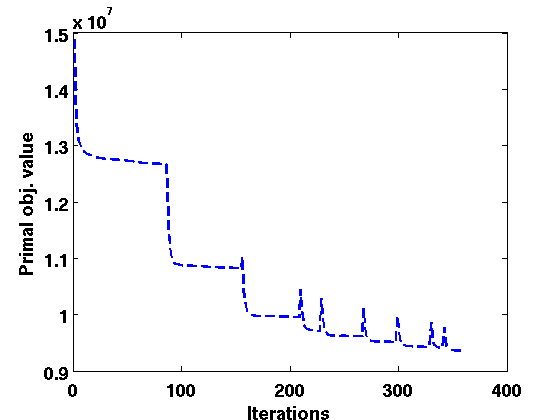
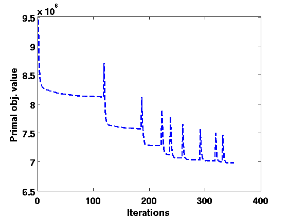
Figure 2: Primal objective value and Test accuracy behaviour for a partition of apartments dataset. The rows correspond to 5, 20 and 100 labeled examples in that order.The square marker in the test accuracy plots denotes the best generalization performance.

5.3 Experiments on the apartments data

Experiments were performed on the apartments dataset with five partitions each for 5,20 and 100 labeled examples. 1000 unlabeled examples were considered and a test set of 100 examples was used to measure the generalization performance. The parameter $C_{l}$ was tuned using a development dataset of 100 examples. The average test set accuracy comparison is presented in Table 3. For apartments dataset, though the features and constraints used in our experiments were the same as those considered in (Dhillon et al., 2012), our data partitions differ from those used in their paper. However, the comparison of mean test accuracy over the 5 different partitions for various split sizes is justified. Note also that we do not include the results with respect to Trans-SSVM for some of our experiments, as different split-sizes are considered for Trans-SSVM in (Yu, 2012). In particular, Yu (2012) considered splits of 10, 25 and 100 labeled examples for their experiments.

The results in Table 3 show that SSVM-SDM achieves a comparable average performance with DASO on all datasets. The plots on test accuracy and primal objective value for various partition sizes are given in Figure 2. The plots show a similar performance as seen for the citation datasets.

6 Conclusion

In this paper, we considered semi-supervised structural SVMs and proposed a simple and efficient algorithm to solve the resulting optimization problem. This involves solving two sub-problems alternately. One of the sub-problems is a simple supervised learning, performed by fixing the labels of the unlabeled training examples. The other sub-problem is the constraint matching problem in which suitable labeling for unlabeled examples are obtained. This was done by an efficient and effective hill-climbing procedure, which ensures that most of the domain constraints are satisfied. The alternating optimization was coupled with deterministic annealing to avoid poor local minima. The proposed algorithm is easy to implement and gives comparable generalization performance. Experimental results on real-world datasets demonstrated that the proposed algorithm is a useful alternative for semi-supervised structured output learning. The proposed label-switching method can also be used to handle complex constraints, which are imposed over only parts of the structured output. We are currently investigating this extension.

References

- Balamurugan et al. (2011) Balamurugan, P., Shevade, S. K., Sundararajan, S., and Keerthi, S. S. (2011). A sequential dual method for structural svms. Proceedings of the Eleventh SIAM International Conference on Data Mining, pages 223–234.
- Bellare et al. (2009) Bellare, K., Druck, G., and McCallum, A. (2009). Alternating projections for learning with expectation constraints optimization. AAAI 2000, pages 43–50. Arlington, Virginia, United States: AUAI Press.
- Chang et al. (2013) Chang, K.-W., Sundararajan, S., and Keerthi, S. S. (2013). Tractable semi-supervised learning of complex structured prediction models. In ECML/PKDD (3), pages 176–191.
- Chang et al. (2007) Chang, M. W., Ratinov, L., and Roth, D. (2007). Guiding semi-supervision with constraint-driven learning. In In Proc. of the Annual Meeting of the ACL.
- Chapelle et al. (2010) Chapelle, O., Schlkopf, B., and Zien, A. (2010). Semi-Supervised Learning. The MIT Press, 1st edition.
- Dhillon et al. (2012) Dhillon, P. S., Keerthi, S. S., Bellare, K., Chapelle, O., and Sellamanickam, S. (2012). Deterministic annealing for semi-supervised structured output learning. Journal of Machine Learning Research - Proceedings Track, 22:299–307.
- Ganchev et al. (2010) Ganchev, K., Graça, J., Gillenwater, J., and Taskar, B. (2010). Posterior regularization for structured latent variable models. J. Mach. Learn. Res., 11:2001–2049.
- Grenager et al. (2005) Grenager, T., Klein, D., and Manning, C. D. (2005). Unsupervised learning of field segmentation models for information extraction. In Proceedings of the 43rd Annual Meeting on Association for Computational Linguistics, ACL ’05, pages 371–378, Stroudsburg, PA, USA. Association for Computational Linguistics.
- Joachims (1999) Joachims, T. (1999). Transductive inference for text classification using support vector machines. In Proceedings of the Sixteenth International Conference on Machine Learning, ICML ’99, pages 200–209, San Francisco, CA, USA. Morgan Kaufmann Publishers Inc.
- Joachims et al. (2009) Joachims, T., Finley, T., and Yu, C.-N. J. (2009). Cutting-plane training of structural svms. Mach. Learn., 77(1):27–59.
- Keerthi et al. (2012) Keerthi, S. S., Sellamanickam, S., and Shevade, S. K. (2012). Extension of tsvm to multi-class and hierarchical text classification problems with general losses. In COLING (Posters), pages 1091–1100.
- Yu (2012) Yu, C.-N. (2012). Transductive learning of structural svms via prior knowledge constraints. Journal of Machine Learning Research - Proceedings Track, 22:1367–1376.
- Zien et al. (2007) Zien, A., Brefeld, U., and Scheffer, T. (2007). Transductive support vector machines for structured variables. In Ghahramani, Z., editor, ICML, volume 227 of ACM International Conference Proceeding Series, pages 1183–1190. ACM.