Fast large-scale optimization by unifying
stochastic gradient and quasi-Newton methods

Fast large-scale optimization by unifying stochastic gradient and quasi-Newton methods - Supplemental Material

Abstract

We present an algorithm for minimizing a sum of functions that combines the computational efficiency of stochastic gradient descent (SGD) with the second order curvature information leveraged by quasi-Newton methods. We unify these approaches by maintaining an independent Hessian approximation for each contributing function in the sum. We maintain computational tractability and limit memory requirements even for high dimensional optimization problems by storing and manipulating these quadratic approximations in a shared, time evolving, low dimensional subspace. Each update step requires only a single contributing function or minibatch evaluation (as in SGD), and each step is scaled using an approximate inverse Hessian and little to no adjustment of hyperparameters is required (as is typical for quasi-Newton methods). This algorithm contrasts with earlier stochastic second order techniques that treat the Hessian of each contributing function as a noisy approximation to the full Hessian, rather than as a target for direct estimation. We experimentally demonstrate improved convergence on seven diverse optimization problems. The algorithm is released as open source Python and MATLAB packages.

1 Introduction

A common problem in optimization is to find a vector $\mathbf{x}^{*}\in\mathcal{R}^{M}$ which minimizes a function $F\left(\mathbf{x}\right)$, where $F\left(\mathbf{x}\right)$ is a sum of $N$ computationally cheaper differentiable subfunctions $f_{i}\left(\mathbf{x}\right)$,

$$F\left(\mathbf{x}\right) =\sum_{i=1}^{N}f_{i}\left(\mathbf{x}\right),$$ (1)

$$\mathbf{x}^{*} =\operatornamewithlimits{argmin}_{\mathbf{x}}F\left(\mathbf{x}\right).$$ (2)

Many optimization tasks fit this form (Boyd & Vandenberghe, 2004), including training of autoencoders, support vector machines, and logistic regression algorithms, as well as parameter estimation in probabilistic models. In these cases each subfunction corresponds to evaluating the objective on a separate data minibatch, thus the number of subfunctions $N$ would be the datasize $D$ divided by the minibatch size $S$. This scenario is commonly referred to in statistics as M-estimation (Huber, 1981).

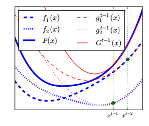
(a)

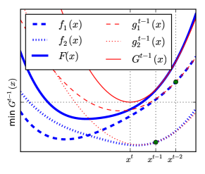
(b)

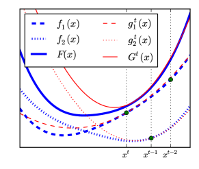
(c)

Figure 1: A cartoon illustrating the proposed optimization technique. (a) The objective function $F\left(x\right)$ (solid blue line) consists of a sum of two subfunctions (dashed blue lines), $F\left(x\right)=f_{1}\left(x\right)+f_{2}\left(x\right)$. At learning step $t-1$, $f_{1}\left(x\right)$ and $f_{2}\left(x\right)$ are approximated by quadratic functions $g^{t-1}_{1}\left(x\right)$ and $g^{t-1}_{2}\left(x\right)$ (red dashed lines). The sum of the approximating functions $G^{t-1}\left(x\right)$ (solid red line) approximates the full objective $F\left(x\right)$. The green dots indicate the parameter values at which each subfunction has been evaluated (b) The next parameter setting $x^{t}$ is chosen by minimizing the approximating function $G^{t-1}\left(x\right)$ from the prior update step. See Equation 4. (c) After each parameter update, the quadratic approximation for one of the subfunctions is updated using a second order expansion around the new parameter vector $x^{t}$. See Equation 12. The constant and first order term in the expansion are evaluated exactly, and the second order term is estimated by performing BFGS on the subfunction’s history. In this case the approximating subfunction $g^{t}_{1}\left(x\right)$ is updated (long-dashed red line). This update is also reflected by a change in the full approximating function $G^{t}\left(x\right)$ (solid red line). Optimization proceeds by repeating these two illustrated update steps. In order to remain tractable in memory and computational overhead, optimization is performed in an adaptive low dimensional subspace determined by the history of gradients and iterates.

There are two general approaches to efficiently optimizing a function of this form. The first is to use a quasi-Newton method (Dennis Jr & Moré, 1977), of which BFGS (Broyden, 1970; Fletcher, 1970; Goldfarb, 1970; Shanno, 1970) or LBFGS (Liu & Nocedal, 1989) are the most common choices. Quasi-Newton methods use the history of gradient evaluations to build up an approximation to the inverse Hessian of the objective function $F\left(\mathbf{x}\right)$. By making descent steps which are scaled by the approximate inverse Hessian, and which are therefore longer in directions of shallow curvature and shorter in directions of steep curvature, quasi-Newton methods can be orders of magnitude faster than steepest descent. Additionally, quasi-Newton techniques typically require adjusting few or no hyperparameters, because they use the measured curvature of the objective function to set step lengths and directions. However, direct application of quasi-Newton methods requires calculating the gradient of the full objective function $F\left(\mathbf{x}\right)$ at every proposed parameter setting $\mathbf{x}$, which can be very computationally expensive.

The second approach is to use a variant of Stochastic Gradient Descent (SGD) (Robbins & Monro, 1951; Bottou, 1991). In SGD, only one subfunction’s gradient is evaluated per update step, and a small step is taken in the negative gradient direction. More recent descent techniques like IAG (Blatt et al., 2007), SAG (Roux et al., 2012), and MISO (Mairal, 2013, 2014) instead take update steps in the average gradient direction. For each update step, they evaluate the gradient of one subfunction, and update the average gradient using its new value. (Bach & Moulines, 2013) averages the iterates rather than the gradients. If the subfunctions are similar, then SGD can also be orders of magnitude faster than steepest descent on the full batch. However, because a different subfunction is evaluated for each update step, the gradients for each update step cannot be combined in a straightforward way to estimate the inverse Hessian of the full objective function. Additionally, efficient optimization with SGD typically involves tuning a number of hyperparameters, which can be a painstaking and frustrating process. (Le et al., 2011) compares the performance of stochastic gradient and quasi-Newton methods on neural network training, and finds both to be competitive.

Combining quasi-Newton and stochastic gradient methods could improve optimization time, and reduce the need to tweak optimization hyperparameters. This problem has been approached from a number of directions. In (Schraudolph et al., 2007; Sunehag et al., 2009) a stochastic variant of LBFGS is proposed. In (Martens, 2010), (Byrd et al., 2011), and (Vinyals & Povey, 2011) stochastic versions of Hessian-free optimization are implemented and applied to optimization of deep networks. In (Lin et al., 2008) a trust region Newton method is used to train logistic regression and linear SVMs using minibatches. In (Hennig, 2013) a nonparametric quasi-Newton algorithm is proposed based on noisy gradient observations and a Gaussian process prior. In (Byrd et al., 2014) LBFGS is performed, but with the contributing changes in gradient and position replaced by exactly computed Hessian vector products computed periodically on extra large minibatches. Stochastic meta-descent (Schraudolph, 1999), AdaGrad (Duchi et al., 2010), and SGD-QN (Bordes et al., 2009) rescale the gradient independently for each dimension, and can be viewed as accumulating something similar to a diagonal approximation to the Hessian. All of these techniques treat the Hessian on a subset of the data as a noisy approximation to the full Hessian. To reduce noise in the Hessian approximation, they rely on regularization and very large minibatches to descend $F\left(\mathbf{x}\right)$. Thus, unfortunately each update step requires the evaluation of many subfunctions and/or yields a highly regularized (i.e. diagonal) approximation to the full Hessian.

We develop a novel second-order quasi-Newton technique that only requires the evaluation of a single subfunction per update step. In order to achieve this substantial simplification, we treat the full Hessian of each subfunction as a direct target for estimation, thereby maintaining a separate quadratic approximation of each subfunction. This approach differs from all previous work, which in contrast treats the Hessian of each subfunction as a noisy approximation to the full Hessian. Our approach allows us to combine Hessian information from multiple subfunctions in a much more natural and efficient way than previous work, and avoids the requirement of large minibatches per update step to accurately estimate the full Hessian. Moreover, we develop a novel method to maintain computational tractability and limit the memory requirements of this quasi-Newton method in the face of high dimensional optimization problems (large $M$). We do this by storing and manipulating the subfunctions in a shared, adaptive low dimensional subspace, determined by the recent history of the gradients and iterates.

Thus our optimization method can usefully estimate and utilize powerful second-order information while simultaneously combatting two potential sources of computational intractability: large numbers of subfunctions (large N) and a high-dimensional optimization domain (large M). Moreover, the use of a second order approximation means that minimal or no adjustment of hyperparameters is required. We refer to the resulting algorithm as Sum of Functions Optimizer (SFO). We demonstrate that the combination of techniques and new ideas inherent in SFO results in faster optimization on seven disparate example problems. Finally, we release the optimizer and the test suite as open source Python and MATLAB packages.

2 Algorithm

Our goal is to combine the benefits of stochastic and quasi-Newton optimization techniques. We first describe the general procedure by which we optimize the parameters $\mathbf{x}$. We then describe the construction of the shared low dimensional subspace which makes the algorithm tractable in terms of computational overhead and memory for large problems. This is followed by a description of the BFGS method by which an online Hessian approximation is maintained for each subfunction. Finally, we end this section with a review of implementation details.

2.1 Approximating Functions

We define a series of functions $G^{t}\left(\mathbf{x}\right)$ intended to approximate $F\left(\mathbf{x}\right)$,

$$G^{t}\left(\mathbf{x}\right)=\sum_{i=1}^{N}g^{t}_{i}\left(\mathbf{x}\right),$$ (3)

where the superscript $t$ indicates the learning iteration. Each $g^{t}_{i}\left(\mathbf{x}\right)$ serves as a quadratic approximation to the corresponding $f_{i}\left(\mathbf{x}\right)$. The functions $g^{t}_{i}\left(\mathbf{x}\right)$ will be stored, and one of them will be updated per learning step.

2.2 Update Steps

As is illustrated in Figure 1, optimization is performed by repeating the steps:

1. Choose a vector $\mathbf{x}^{t}$ by minimizing the approximating objective function $G^{t-1}\left(\mathbf{x}\right)$,

   $$\mathbf{x}^{t}=\operatornamewithlimits{argmin}_{\mathbf{x}}G^{t-1}\left(\mathbf{x}\right).$$ (4)

   Since $G^{t-1}\left(\mathbf{x}\right)$ is a sum of quadratic functions $g_{i}^{t-1}\left(\mathbf{x}\right)$, it can be exactly minimized by a Newton step,

   $$\mathbf{x}^{t}=\mathbf{x}^{t-1}-\eta^{t}\left(\mathbf{H}^{t-1}\right)^{-1}\frac{\partial G^{t-1}\left(\mathbf{x}^{t-1}\right)}{\partial\mathbf{x}},$$ (5)

   where $\mathbf{H}^{t-1}$ is the Hessian of $G^{t-1}\left(\mathbf{x}\right)$. The step length $\eta^{t}$ is typically unity, and will be discussed in Section 3.5.

2. Choose an index $j\in\{1...N\}$, and update the corresponding approximating subfunction $g_{i}^{t}\left(\mathbf{x}\right)$ using a second order power series around $\mathbf{x}^{t}$, while leaving all other subfunctions unchanged,

$$g_{i}^{t}\left(\mathbf{x}\right)=\left\{\begin{array}[]{lcrl}g_{i}^{t-1}\left(\mathbf{x}\right)&&i\neq j\\ \\ \left[\begin{array}[]{l}f_{i}\left(\mathbf{x}^{t}\right)\\ \quad+\left(\mathbf{x}-\mathbf{x}^{t}\right)^{T}{f^{\prime}_{i}\left(\mathbf{x}^{t}\right)}\\ \quad+\frac{1}{2}\left(\mathbf{x}-\mathbf{x}^{t}\right)^{T}\mathbf{H}_{i}^{t}\ \left(\mathbf{x}-\mathbf{x}^{t}\right)\end{array}\right]&&i=j&\end{array}\right..$$ (12)

The constant and first order term in Equation 12 are set by evaluating the subfunction and gradient, $f_{j}\left(\mathbf{x}^{t}\right)$ and $f^{\prime}_{j}\left(\mathbf{x}^{t}\right)$. The quadratic term $\mathbf{H}_{j}^{t}$ is set by using the BFGS algorithm to generate an online approximation to the true Hessian of subfunction $j$ based on its history of gradient evaluations (see Section 2.4). The Hessian of the summed approximating function $G^{t}\left(\mathbf{x}\right)$ in Equation 5 is the sum of the Hessians for each $g^{t}_{j}\left(\mathbf{x}\right)$, $\mathbf{H}^{t}=\sum_{j}\mathbf{H}^{t}_{j}$.

2.3 A Shared, Adaptive, Low-Dimensional Representation

The dimensionality $M$ of $\mathbf{x}\in\mathcal{R}^{M}$ is typically large. As a result, the memory and computational cost of working directly with the matrices $\mathbf{H}_{i}^{t}\in\mathcal{R}^{M\times M}$ is typically prohibitive, as is the cost of storing the history terms $\Delta{f^{\prime}}$ and $\Delta\mathbf{x}$ required by BFGS (see Section 2.4). To reduce the dimensionality from $M$ to a tractable value, all history is instead stored and all updates computed in a lower dimensional subspace, with dimensionality between $K_{min}$ and $K_{max}$. This subspace is constructed such that it includes the most recent gradient and position for every subfunction, and thus $K_{min}\geq 2N$. This guarantees that the subspace includes both the steepest gradient descent direction over the full batch, and the update directions from the most recent Newton steps (Equation 5).

For the results in this paper, $K_{min}=2N$ and $K_{max}=3N$. The subspace is represented by the orthonormal columns of a matrix $\mathbf{P}^{t}\in\mathcal{R}^{M\times K^{t}}$, $\left(\mathbf{P}^{t}\right)^{T}\mathbf{P}^{t}=\mathbf{I}$. $K^{t}$ is the subspace dimensionality at optimization step $t$.

2.3.1 Expanding the Subspace with a New Observation

At each optimization step, an additional column is added to the subspace, expanding it to include the most recent gradient direction. This is done by first finding the component in the gradient vector which lies outside the existing subspace, and then appending that component to the current subspace,

$$\mathbf{q}_{\text{orth}} =f^{\prime}_{j}\left(\mathbf{x}^{t}\right)-\mathbf{P}^{t-1}\left(\mathbf{P}^{t-1}\right)^{T}f^{\prime}_{j}\left(\mathbf{x}^{t}\right),$$ (13)

$$\mathbf{P}^{t} =\left[\mathbf{P}^{t-1}\quad\frac{\mathbf{q}_{\text{orth}}}{\left|\left|\mathbf{q}_{\text{orth}}\right|\right|}\right],$$ (14)

where $j$ is the subfunction updated at time $t$. The new position $\mathbf{x}^{t}$ is included automatically, since the position update was computed within the subspace $\mathbf{P}^{t-1}$. Vectors embedded in the subspace $\mathbf{P}^{t-1}$ can be updated to lie in $\mathbf{P}^{t}$ simply by appending a $0$, since the first $K^{t-1}$ dimensions of $\mathbf{P}^{t}$ consist of $\mathbf{P}^{t-1}$.

2.3.2 Restricting the Size of the Subspace

In order to prevent the dimensionality $K^{t}$ of the subspace from growing too large, whenever $K^{t}>K_{max}$, the subspace is collapsed to only include the most recent gradient and position measurements from each subfunction. The orthonormal matrix representing this collapsed subspace is computed by a QR decomposition on the most recent gradients and positions. A new collapsed subspace is thus computed as,

$$\mathbf{P}^{\prime} =\text{orth}\left(\left[f^{\prime}_{1}\left(\mathbf{x}^{\tau_{1}^{t}}\right)\cdots f^{\prime}_{N}\left(\mathbf{x}^{\tau_{N}^{t}}\right)\quad\mathbf{x}^{\tau_{1}^{t}}\cdots\mathbf{x}^{\tau_{N}^{t}}\right]\right),$$ (15)

where $\tau_{i}^{t}$ indicates the learning step at which the $i$th subfunction was most recently evaluated, prior to the current learning step $t$. Vectors embedded in the prior subspace $\mathbf{P}$ are projected into the new subspace $\mathbf{P}^{\prime}$ by multiplication with a projection matrix $\mathbf{T}=\left(\mathbf{P}^{\prime}\right)^{T}\mathbf{P}$. Vector components which point outside the subspace defined by the most recent positions and gradients are lost in this projection.

Note that the subspace $\mathbf{P}^{\prime}$ lies within the subspace $\mathbf{P}$. The QR decomposition and the projection matrix $\mathbf{T}$ are thus both computed within $\mathbf{P}$, reducing the computational and memory cost (see Section 4.1).

2.4 Online Hessian Approximation

An independent online Hessian approximation $\mathbf{H}_{j}^{t}$ is maintained for each subfunction $j$. It is computed by performing BFGS on the history of gradient evaluations and positions for that single subfunction.

2.4.1 History Matrices

For each subfunction $j$, we construct two matrices, $\Delta{f^{\prime}}$ and $\Delta\mathbf{x}$. Each column of $\Delta{f^{\prime}}$ holds the change in the gradient of subfunction $j$ between successive evaluations of that subfunction, including all evaluations up until the present time. Each column of $\Delta\mathbf{x}$ holds the corresponding change in the position $\mathbf{x}$ between successive evaluations. Both matrices are truncated after a number of columns $L$, meaning that they include information from only the prior $L+1$ gradient evaluations for each subfunction. For all results in this paper, $L=10$ (identical to the default history length for the LBFGS implementation used in Section 5).

2.4.2 BFGS Updates

The BFGS algorithm functions by iterating through the columns in $\Delta{f^{\prime}}$ and $\Delta\mathbf{x}$, from oldest to most recent. Let $s$ be a column index, and $\mathbf{B}_{s}$ be the approximate Hessian for subfunction $j$ after processing column $s$. For each $s$, the approximate Hessian matrix $\mathbf{B}_{s}$ is set so that it obeys the secant equation $\Delta{f^{\prime}}_{s}=\mathbf{B}_{s}\Delta\mathbf{x}_{s}$, where $\Delta{f^{\prime}}_{s}$ and $\Delta\mathbf{x}_{s}$ are taken to refer to the $s$th columns of the gradient difference and position difference matrix respectively.

In addition to satisfying the secant equation, $\mathbf{B}_{s}$ is chosen such that the difference between it and the prior estimate $\mathbf{B}_{s-1}$ has the smallest weighted Frobenius norm. This produces the standard BFGS update equation

$$\mathbf{B}_{s} =\mathbf{B}_{s-1}+\frac{\Delta{f^{\prime}}_{s}\Delta{f^{\prime}}_{s}^{T}}{\Delta{f^{\prime}}_{s}^{T}\Delta\mathbf{x}_{s}}-\frac{\mathbf{B}_{s-1}\Delta\mathbf{x}_{s}\Delta\mathbf{x}_{s}^{T}\mathbf{B}_{s-1}}{\Delta\mathbf{x}_{s}^{T}\mathbf{B}_{s-1}\Delta\mathbf{x}_{s}}.$$ (16)

The final update is used as the approximate Hessian for subfunction $j$, $\mathbf{H}_{j}^{t}=\mathbf{B}_{\max(s)}$.

Optimizer	Computation per pass	Memory use
SFO	$\mathcal{O}\left(QN+MN^{2}\right)$	$\mathcal{O}\left(MN\right)$
SFO, ‘sweet spot’	$\mathcal{O}\left(QN\right)$	$\mathcal{O}\left(MN\right)$
LBFGS	$\mathcal{O}\left(QN+ML\right)$	$\mathcal{O}\left(ML\right)$
SGD	$\mathcal{O}\left(QN\right)$	$\mathcal{O}\left(M\right)$
AdaGrad	$\mathcal{O}\left(QN\right)$	$\mathcal{O}\left(M\right)$
SAG	$\mathcal{O}\left(QN\right)$	$\mathcal{O}\left(MN\right)$

Table 1: Leading terms in the computational cost and memory requirements for SFO and several competing algorithms. $Q$ is the cost of computing the value and gradient for a single subfunction, $M$ is the number of data dimensions, $N$ is the number of subfunctions, and $L$ is the number of history terms retained. “SFO, ‘sweet spot”’ refers to the case discussed in Section 4.1.1 where the minibatch size is adjusted to match computational overhead to subfunction evaluation cost. For this table, it is assumed that $M\gg N\gg L$.

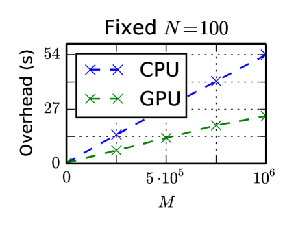
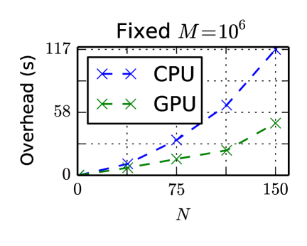
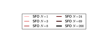
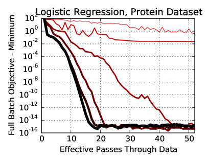
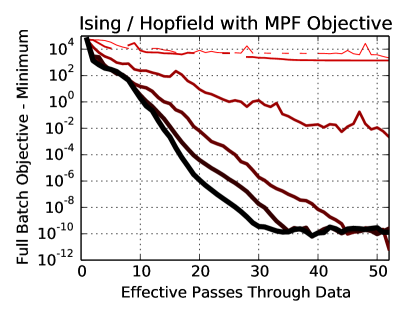
(a)                                                               (b) (c)

Figure 2: An exploration of computational overhead and optimizer performance, especially as the number of minibatches or subfunctions $N$ is adjusted. (a) Computational overhead required by SFO for a full pass through all the subfunctions as a function of dimensionality $M$ for fixed $N=100$. (b) Computational overhead of SFO as a function of $N$ for fixed $M=10^{6}$. Both plots show the computational time required for a full pass of the optimizer, excluding time spent computing the target objective and gradient. This time is dominated by the $\mathcal{O}\left(MN^{2}\right)$ cost per pass of $N$ iterations of subspace projection. CPU indicates that all computations were performed on a 2012 Intel i7-3970X CPU (6 cores, 3.5 GHz). GPU indicates that subspace projection was performed on a GeForce GTX 660 Ti GPU. (c) Optimization performance on the two convex problems in Section 5 as a function of the number of minibatches $N$. Note that near maximal performance is achieved after breaking the target problem into only a small number of minibatches.

3 Implementation Details

Here we briefly review additional design choices that were made when implementing this algorithm. Each of these choices is presented more thoroughly in Appendix C. Supplemental Figure C.1 demonstrates that the optimizer performance is robust to changes in several of these design choices.

3.1 BFGS Initialization

The first time a subfunction is evaluated (before there is sufficient history to run BFGS), the approximate Hessian $\mathbf{H}_{j}^{t}$ is set to the identity times the median eigenvalue of the average Hessian of the other active subfunctions. For later evaluations, the initial BFGS matrix is set to a scaled identity matrix, $\mathbf{B}_{0}=\beta\mathbf{I}$, where $\beta$ is the minimum eigenvalue found by solving the squared secant equation for the full history. See Appendix C.1 for details and motivation.

3.2 Enforcing Positive Definiteness

It is typical in quasi-Newton techniques to enforce that the Hessian approximation remain positive definite. In SFO each $\mathbf{H}^{t}_{i}$ is constrained to be positive definite by an explicit eigendecomposition and setting any too-small eigenvalues to the median positive eigenvalue. This is computationally cheap due to the shared low dimensional subspace (Section 2.3). This is described in detail in Appendix C.2.

3.3 Choosing a Target Subfunction

The subfunction $j$ to update in Equation 12 is chosen to be the one farthest from the current location $\mathbf{x}^{t}$, using the current Hessian approximation as the metric. This is described more formally in Appendix C.3. As illustrated in Supplemental Figure C.1, this distance based choice outperforms the commonly used random choice of subfunction.

3.4 Growing the Number of Active Subfunctions

For many problems of the form in Equation 1, the gradient information is nearly identical between the different subfunctions early in learning. We therefore begin with only two active subfunctions, and expand the active set whenever the length of the standard error in the gradient across subfunctions exceeds the length of the gradient. This process is described in detail in Appendix C.4. As illustrated in Supplemental Figure C.1, performance only differs from the case where all subfunctions are initially active for the first several optimization passes.

3.5 Detecting Bad Updates

Small eigenvalues in the Hessian can cause update steps to overshoot severely (ie, if higher than second order terms come to dominate within a distance which is shorter than the suggested update step). It is therefore typical in quasi-Newton methods such as BFGS, LBFGS, and Hessian-free optimization to detect and reject bad proposed update steps, for instance by a line search. In SFO, bad update steps are detected by comparing the measured subfunction value $f_{j}\left(\mathbf{x}^{t}\right)$ to its quadratic approximation $g_{j}^{t-1}\left(\mathbf{x}^{t}\right)$. This is discussed in detail in Section C.5.

4 Properties

4.1 Computational Overhead and Storage Cost

Table 1 compares the cost of SFO to competing algorithms. The dominant computational costs are the $\mathcal{O}\left(MN\right)$ cost of projecting the $M$ dimensional gradient and current parameter values into and out of the $\mathcal{O}\left(N\right)$ dimensional active subspace for each learning iteration, and the $\mathcal{O}\left(Q\right)$ cost of evaluating a single subfunction. The dominant memory cost is $\mathcal{O}\left(MN\right)$, and stems from storing the active subspace $\mathbf{P}^{t}$. Table A.1 in the Supplemental Material provides the contribution to the computational cost of each component of SFO. Figure 2 plots the computational overhead per a full pass through all the subfunctions associated with SFO as a function of $M$ and $N$. If each of the $N$ subfunctions corresponds to a minibatch, then the computational overhead can be shrunk as described in Section 4.1.1.

Without the low dimensional subspace, the leading term in the computational cost of SFO would be the far larger $\mathcal{O}\left(M^{2.4}\right)$ cost per iteration of inverting the approximate Hessian matrix in the full $M$ dimensional parameter space, and the leading memory cost would be the far larger $\mathcal{O}\left(M^{2}N\right)$ from storing an $M\times M$ dimensional Hessian for all $N$ subfunctions.

4.1.1 Ideal Minibatch Size

Many objective functions consist of a sum over a number of data points $D$, where $D$ is often larger than $M$. For example, $D$ could be the number of training samples in a supervised learning problem, or data points in maximum likelihood estimation. To control the computational overhead of SFO in such a regime, it is useful to choose each subfunction in Equation 3 to itself be a sum over a minibatch of data points of size $S$, yielding $N=\frac{D}{S}$. This leads to a computational cost of evaluating a single subfunction and gradient of $\mathcal{O}\left(Q\right)=\mathcal{O}\left(MS\right)$. The computational cost of projecting this gradient from the full space to the shared $N$ dimensional adaptive subspace, on the other hand, is $\mathcal{O}\left(MN\right)=\mathcal{O}\left(M\frac{D}{S}\right)$. Therefore, in order for the costs of function evaluation and projection to be the same order, the minibatch size $S$ should be proportional to $\sqrt{D}$, yielding

$$N \propto\sqrt{D}.$$ (17)

The constant of proportionality should be chosen small enough that the majority of time is spent evaluating the subfunction. In most problems of interest, $\sqrt{D}\ll M$, justifying the relevance of the regime in which the number of subfunctions $N$ is much less than the number of parameters $M$. Finally, the computational and memory costs of SFO are the same for sparse and non-sparse objective functions, while Q is often much smaller for a sparse objective. Thus the ideal $S$ ($N$) is likely to be larger (smaller) for sparse objective functions.

Note that as illustrated in Figure 2c and Figure 3 performance is very good even for small $N$.

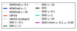
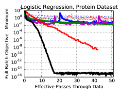
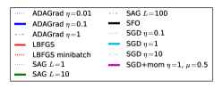
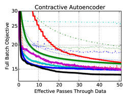
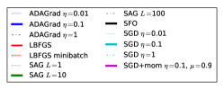
(a)	(b)	(c)
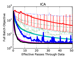
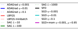
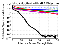
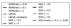
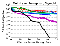
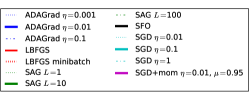
(d)	(e)	(f)

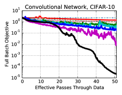
Figure 3: A comparison of SFO to competing optimization techniques for six objective functions. The bold lines indicate the best performing hyperparameter for each optimizer. Note that unlike all other techniques besides LBFGS, SFO does not require tuning hyperparameters (for instance, the displayed SGD+momentum traces are the best out of 32 hyperparameter configurations). The objective functions shown are (a) a logistic regression problem, (b) a contractive autoencoder trained on MNIST digits, (c) an Independent Component Analysis (ICA) model trained on MNIST digits, (d) an Ising model / Hopfield associative memory trained using Minimum Probability Flow, (e) a multi-layer perceptron with sigmoidal units trained on MNIST digits, and (f) a multilayer convolutional network with rectified linear units trained on CIFAR-10. The logistic regression and MPF Ising objectives are convex, and their objective values are plotted relative to the global minimum.

4.2 Convergence

Concurrent work by (Mairal, 2013) considers a similar algorithm to that described in Section 2.2, but with $\mathbf{H}_{i}^{t}$ a scalar constant rather than a matrix. Proposition 6.1 in (Mairal, 2013) shows that in the case that each $g_{i}$ majorizes its respective $f_{i}$, and subject to some additional smoothness constraints, $G^{t}\left(\mathbf{x}\right)$ monotonically decreases, and $\mathbf{x}^{*}$ is an asymptotic stationary point. Proposition 6.2 in (Mairal, 2013) further shows that for strongly convex $f_{i}$, the algorithm exhibits a linear convergence rate to $\mathbf{x}^{*}$. A near identical proof should hold for a simplified version of SFO, with random subfunction update order, and with $\mathbf{H}_{i}^{t}$ regularized in order to guarantee satisfaction of the majorization condition.

5 Experimental Results

We compared our optimization technique to several competing optimization techniques for seven objective functions. The results are illustrated in Figures 3 and 4, and the optimization techniques and objectives are described below. For all problems our method outperformed all other techniques in the comparison.

Open source code which implements the proposed technique and all competing optimizers, and which directly generates the plots in Figures 1, 2, and 3, is provided at https://github.com/Sohl-Dickstein/Sum-of-Functions-Optimizer.

5.1 Optimizers

SFO refers to Sum of Functions Optimizer, and is the new algorithm presented in this paper. SAG refers to Stochastic Average Gradient method, with the trailing number providing the Lipschitz constant. SGD refers to Stochastic Gradient Descent, with the trailing number indicating the step size. ADAGrad indicates the AdaGrad algorithm, with the trailing number indicating the initial step size. LBFGS refers to the limited memory BFGS algorithm. LBFGS minibatch repeatedly chooses one tenth of the subfunctions, and runs LBFGS for ten iterations on them. Hessian-free refers to Hessian-free optimization.

For SAG, SGD, and ADAGrad the hyperparameter was chosen by a grid search. The best hyperparameter value, and the hyperparameter values immediately larger and smaller in the grid search, are shown in the plots and legends for each model in Figure 3. In SGD+momentum the two hyperparameters for both step size and momentum coefficient were chosen by a grid search, but only the best parameter values are shown. The grid-searched momenta were 0.5, 0.9, 0.95, and 0.99, and the grid-searched step lengths were all integer powers of ten between $10^{-5}$ and $10^{2}$. For Hessian-free, the hyperparameters, source code, and objective function are identical to those used in (Martens, 2010), and the training data was divided into four “chunks.” For all other experiments and optimizers the training data was divided into $N=100$ minibatches (or subfunctions).

5.2 Objective Functions

A detailed description of all target objective functions in Figure 3 is included in Section B of the Supplemental Material. In brief, they consisted of:

• A logistic regression objective, chosen to be the same as one used in (Roux et al., 2012).

• A contractive autoencoder with 784 visible units, and 256 hidden units, similar to the one in (Rifai et al., 2011).

• An Independent Components Analysis (ICA) (Bell & Sejnowski, 1995) model with Student’s t-distribution prior.

• An Ising model / Hopfield network trained using code from (Hillar et al., 2012) implementing MPF (Sohl-Dickstein et al., 2011b, a).

• A multilayer perceptron with a similar architecture to (Hinton et al., 2012), with layer sizes of 784, 1200, 1200, and 10. Training used Theano (Bergstra & Breuleux, 2010).

• A deep convolutional network with max pooling and rectified linear units, similar to (Goodfellow & Warde-Farley, 2013a), with two convolutional layers with 48 and 128 units, and one fully connected layer with 240 units. Training used Theano and Pylearn2 (Goodfellow & Warde-Farley, 2013b).

The logistic regression and Ising model / Hopfield objectives are convex, and are plotted relative to their global minimum. The global minimum was taken to be the smallest value achieved on the objective by any optimizer.

In Figure 4, a twelve layer neural network was trained on cross entropy reconstruction error for the CURVES dataset. This objective, and the parameter initialization, was chosen to be identical to an experiment in (Martens, 2010).

6 Future Directions

We perform optimization in an $\mathcal{O}\left(N\right)$ dimensional subspace. It may be possible, however, to drastically reduce the dimensionality of the active subspace without significantly reducing optimization performance. For instance, the subspace could be determined by accumulating, in an online fashion, the leading eigenvectors of the covariance matrix of the gradients of the subfunctions, as well as the leading eigenvectors of the covariance matrix of the update steps. This would reduce memory requirements and computational overhead even for large numbers of subfunctions (large $N$).

Most portions of the presented algorithm are naively parallelizable. The $g_{i}^{t}\left(\mathbf{x}\right)$ functions can be updated asynchronously, and can even be updated using function and gradient evaluations from old positions $\mathbf{x}^{\tau}$, where $\tau<t$. Developing a parallelized version of this algorithm could make it a useful tool for massive scale optimization problems. Similarly, it may be possible to adapt this algorithm to an online / infinite data context by replacing subfunctions in a rolling fashion.

Quadratic functions are often a poor match to the geometry of the objective function (Pascanu et al., 2012). Neither the dynamically updated subspace nor the use of independent approximating subfunctions $g_{i}^{t}\left(\mathbf{x}\right)$ which are fit to the true subfunctions $f_{i}\left(\mathbf{x}\right)$ depend on the functional form of $g_{i}^{t}\left(\mathbf{x}\right)$. Exploring non-quadratic approximating subfunctions has the potential to greatly improve performance.

Section 3.1 initializes the approximate Hessian using a diagonal matrix. Instead, it might be effective to initialize the approximate Hessian for each subfunction using the average approximate Hessian from all other subfunctions. Where individual subfunctions diverged they would overwrite this initialization. This would take advantage of the fact that the Hessians for different subfunctions are very similar for many objective functions.

Recent work has explored the non-asymptotic convergence properties of stochastic optimization algorithms (Bach & Moulines, 2011). It may be fruitful to pursue a similar analysis in the context of SFO.

Finally, the natural gradient (Amari, 1998) can greatly accelerate optimization by removing the effect of dependencies and relative scalings between parameters. The natural gradient can be simply combined with other optimization methods by performing a change of variables, such that in the new parameter space the natural gradient and the ordinary gradient are identical (Sohl-Dickstein, 2012). It should be straightforward to incorporate this change-of-variables technique into SFO.

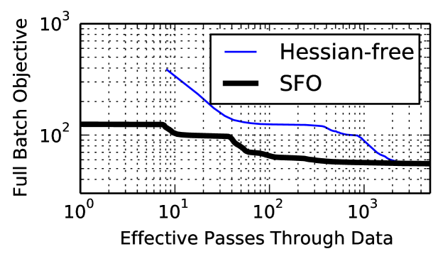
Figure 4: A comparison of SFO to Hessian-free optimization for a twelve layer neural network trained on the CURVES dataset. This problem is identical to an experiment in (Martens, 2010), and the Hessian-free convergence trace was generated using source code from the same paper. SFO converges in approximately one tenth the number of effective passes through the data as Hessian-free optimization.

7 Conclusion

We have presented an optimization technique which combines the benefits of LBFGS-style quasi-Newton optimization and stochastic gradient descent. It does this by using BFGS to maintain an independent quadratic approximation for each contributing subfunction (or minibatch) in an objective function. Each optimization step then alternates between descending the quadratic approximation of the full objective, and evaluating a single subfunction and updating the quadratic approximation for that single subfunction. This procedure is made tractable in memory and computational time by working in a shared low dimensional subspace defined by the history of gradient evaluations.

Appendix A Computational Complexity

Here we provide a description of the computational cost of each component of the SFO algorithm. See Table A.1. The computational cost of matrix multiplication for $N\times N$ matrices is taken to be $\mathcal{O}\left(N^{2.4}\right)$.

A.1 Function and Gradient Computation

By definition, the cost of computing the function value and gradient for each subfunction is $\mathcal{O}\left(Q\right)$, and this must be done $N$ times to complete a full effective pass through all the subfunctions, yielding a total cost per pass of $\mathcal{O}\left(QN\right)$.

A.2 Subspace Projection

Once per iteration, the updated parameter values $\mathbf{x}^{t}$ must be projected from the $N$ dimensional adaptive low dimensional subspace into the full $M$ dimensional parameter space. Similarly, once per iteration the gradient must be projected from the full $M$ dimensional parameter space into the $N$ dimensional subspace. See Section 2.3. Additionally the residual of the gradient projection must be appended to the subspace as described in Equation 14. Each of these operations has cost $\mathcal{O}\left(MN\right)$, stemming from multiplication of a parameter or gradient vector by the subspace matrix $\mathbf{P}^{t}$. They are performed $N$ times per effective pass through the data, yielding a total cost per pass of $\mathcal{O}\left(MN^{2}\right)$.

A.3 Subspace Collapse

In order to constrain the dimensionality $K^{t}$ of the subspace to remain order $\mathcal{O}\left(N\right)$, the subspace must be collapsed every $\mathcal{O}\left(N\right)$ steps, or $\mathcal{O}\left(1\right)$ times per pass. This is described in Section 2.3.2. The collapsed subspace is computed using a QR decomposition on the history terms (see Equation 15) within the current subspace, with computational complexity $\mathcal{O}\left(N^{3}\right)$. The old subspace matrix $\mathbf{P}$ is then projected into the new subspace matrix $\mathbf{P}^{\prime}$, involving the multiplication of a $\mathcal{O}\left(M\times N\right)$ matrix with a $\mathcal{O}\left(N\times N\right)$ projection matrix, with corresponding complexity $\mathcal{O}\left(MN^{1.4}\right)$. The total complexity per pass is thus $O\left(MN^{1.4}+N^{3}\right)$.

A.4 Minimize $G^{t}\left(\mathbf{x}\right)$

$G^{t}\left(\mathbf{x}\right)$ is minimized by an explicit matrix inverse in Equation 5. Computing this inverse has cost $\mathcal{O}\left(N^{2.4}\right)$, and must be performed $N$ times per effective pass through the data.

With only small code changes, this inverse could instead be updated each iteration using the Woodbury identity and the inverse from the prior step, with cost $\mathcal{O}\left(N^{2}\right)$. However, minimization of $G^{t}\left(\mathbf{x}\right)$ is not a leading contributor to the overall computational cost, and so increasing its efficiency would have little effect.

A.5 BFGS

The BFGS iterations are performed in the $\mathcal{O}\left(L\right)$ dimensional subspace defined by the columns of $\Delta{f^{\prime}}$ and $\Delta\mathbf{x}$. Since BFGS consists of $L$ rank two updates of an $\mathcal{O}\left(L\times L\right)$ matrix, the cost of performing BFGS iterations is $\mathcal{O}\left(L^{3}\right)$. See Section 2.4.2. The cost of using a QR decomposition to compute the $L$ dimensional subspace defined by the columns of $\Delta{f^{\prime}}$ and $\Delta\mathbf{x}$ is $\mathcal{O}\left(NL^{2}\right)$, and the cost of projecting the $L$ history terms of length $N$ into the subspace is $\mathcal{O}\left(NL^{1.4}\right)$. BFGS is performed $N$ times per effective pass through the data. The total cost of BFGS is therefore $\mathcal{O}\left(N^{2}L^{2}+NL^{3}\right)$.

In the current implementation, the full BFGS chain for a subfunction is recomputed every iteration. However, BFGS could be modified to only compute the rank two update to the prior Hessian approximation at each iteration. This would sacrifice the history-dependent initialization described in Section 3.1. The resulting complexity per iteration would instead be $\mathcal{O}\left(N^{2}\right)$, and the computational complexity per pass would instead be $\mathcal{O}\left(N^{3}\right)$. BFGS is also not a leading contributor to the overall computational cost, and so increasing its efficiency would have little effect.

Appendix B Objective Functions

A more detailed description of the objective functions used for experiments in the main text follows.

B.1 Logistic Regression

We chose the logistic regression objective, L2 regularization penalty, and training dataset to be identical to the protein homology test case in the recent Stochastic Average Gradient paper (Roux et al., 2012), to allow for direct comparison of techniques. The one difference is that our total objective function is divided by the number of samples per minibatch, but unlike in (Roux et al., 2012) is not also divided by the number of minibatches. This different scaling places the hyperparameters for all optimizers in the same range as for our other experiments.

B.2 Autoencoder

We trained a contractive autoencoder, which penalizes the Frobenius norm of the Jacobian of the encoder function, on MNIST digits. Autoencoders of this form have been successfully used for learning deep representations in neural networks (Rifai et al., 2011). Sigmoid nonlinearities were used for both encoder and decoder. The regularization penalty was set to 1, and did not depend on the number of hidden units. The reconstruction error was divided by the number of training examples per minibatch. There were 784 visible units, and 256 hidden units.

B.3 Independent Components Analysis

We trained an Independent Components Analysis (ICA) (Bell & Sejnowski, 1995) model with Student’s t-distribution prior on MNIST digits by minimizing the negative log likelihood of the ICA model under the digit images. Both the receptive fields and the Student’s t shape parameter were estimated. Digit images were preprocessed by performing PCA whitening and discarding components with variance less than $10^{-4}$ times the maximum variance. The objective function was divided by the number of training examples per minibatch.

B.4 Ising Model / Hopfield Network via MPF

We trained an Ising/Hopfield model on MNIST digits, using code from (Hillar et al., 2012). Optimal Hopfield network storage capacity can be achieved by training the corresponding Ising model via MPF (Hillar et al., 2012; Sohl-Dickstein et al., 2011b, a). The MPF objective was divided by the number of training examples per minibatch. An L2 regularization penalty with coefficient 0.01 was added to the objective for each minibatch.

B.5 Multilayer Perceptron

We trained a deep neural network to classify digits on the MNIST digit recognition benchmark. We used a similar architecture to (Hinton et al., 2012). Our network consisted of: 784 input units, one hidden layer of 1200 units, a second hidden layer of 1200 units, and 10 output units. We ran the experiment using both rectified linear and sigmoidal units. The objective used was the standard softmax regression on the output units. Theano (Bergstra & Breuleux, 2010) was used to implement the model architecture and compute the gradient.

B.6 Deep Convolutional Network

We trained a deep convolutional network on CIFAR-10 using max pooling and rectified linear units. The architecture we used contains two convolutional layers with 48 and 128 units respectively, followed by one fully connected layer of 240 units. This architecture was loosely based on (Goodfellow & Warde-Farley, 2013a). Pylearn2 (Goodfellow & Warde-Farley, 2013b) and Theano were used to implement the model.

Appendix C Implementation Details

Here we expand on the implementation details which are outlined in Section 3 in the main text. Figure C.1 provides empirical motivation for several of the design choices made in this paper, by showing the change in convergence traces when those design choices are changed. Note that even when these design choices are changed, convergence is still more rapid than for the competing techniques in Figure 3.

C.1 BFGS Initialization

No History

An approximate Hessian can only be computed as described in Section 2.4 after multiple gradient evaluations. If a subfunction $j$ only has one gradient evaluation, then its approximate Hessian $\mathbf{H}_{j}^{t}$ is set to the identity times the median eigenvalue of the average Hessian of the other active subfunctions. If $j$ is the very first subfunction to be evaluated, $\mathbf{H}_{j}^{t}$ is initialized as the identity matrix times a large positive constant ($10^{6}$).

The First BFGS Step

The initial approximate Hessian matrix used in BFGS is set to a scaled identity matrix, so that $\mathbf{B}_{0}=\beta\mathbf{I}$. This initialization will be overwritten by Equation 16 for all explored directions. It’s primary function, then, is to set the estimated Hessian for unexplored directions. Gradient descent routines tend to progress from directions with large slopes and curvatures, and correspondingly large eigenvalues, to directions with shallow slopes and curvatures, and smaller eigenvalues. The typical eigenvalue in an unexplored direction is thus expected to be smaller than in previously explored directions. We therefore set $\beta$ using a measure of the smallest eigenvalue in an explored direction

The scaling factor $\beta$ is set to the smallest non-zero eigenvalue of a matrix $\mathbf{Q}$, $\beta=\min_{\lambda_{Q}>0}\lambda_{Q}$, where $\lambda_{Q}$ indicates the eigenvalues of $\mathbf{Q}$. $\mathbf{Q}$ is the symmetric matrix with the smallest Frobenius norm which is consistent with the squared secant equations for all columns in $\Delta{f^{\prime}}$ and $\Delta\mathbf{x}$. That is,

$$\mathbf{Q} =\left[{{\left(\Delta\mathbf{x}\right)}^{+}}^{T}{\left(\Delta{f^{\prime}}\right)}^{T}\Delta{f^{\prime}}{\left(\Delta\mathbf{x}\right)}^{+}\right]^{\frac{1}{2}},$$ (18)

where ⁺ indicates the pseudoinverse, and $\frac{1}{2}$ indicates the matrix square root. All of the eigenvalues of $\mathbf{Q}$ are non-negative. $\mathbf{Q}$ and $\lambda_{Q}$ are computed in the subspace defined by $\Delta{f^{\prime}}$ and $\Delta\mathbf{x}$, reducing computational cost (see Section 4.1).

C.2 Enforcing Positive Definiteness

It is typical in quasi-Newton techniques to enforce that the Hessian approximation remain positive definite. In SFO, at the end of the BFGS procedure, each $\mathbf{H}^{t}_{i}$ is constrained to be positive definite by performing an eigendecomposition, and setting any eigenvalues which are too small to the median positive eigenvalue. The median is used because it provides a measure of “typical” curvature. When an eigenvalue is negative (or extremely close to 0), it provides a poor estimate of curvature over the interval required to reach a minimum in the direction of the corresponding eigenvector. Replacing it with the median eigenvalue therefore provides a more reasonable estimate. If $\lambda_{max}$ is the maximum eigenvalue of $\mathbf{H}^{t}_{i}$, then any eigenvalues smaller than $\gamma\lambda_{max}$ are set to be equal to $\operatornamewithlimits{median}_{\lambda>0}\lambda$. For all experiments shown here, $\gamma=10^{-8}$. As described in Section 2.3, a shared low dimensional representation makes this eigenvalue computation tractable.

C.3 Choosing a Target Subfunction

The subfunction $j$ to update in Equation 12 is chosen as,

$$j =\operatornamewithlimits{argmax}_{i}\left[\mathbf{x}^{t}-\mathbf{x}^{\tau_{i}}\right]^{T}\mathbf{Q}^{t}\left[\mathbf{x}^{t}-\mathbf{x}^{\tau_{i}}\right],$$ (19)

where $\tau_{i}$ indicates the time at which subfunction $i$ was last evaluated, and $\mathbf{Q}$ is either set to either $\mathbf{H}_{i}^{t}$ or $\mathbf{H}^{t}$, with probability $\frac{1}{2}$ for each.

That is, the updated subfunction is the one which was last evaluated farthest from the current location, using the approximate Hessian as a metric. This is motivated by the observation that the approximating functions which were computed farthest from the current location tend to be the functions which are least accurate at the current location, and therefore the most useful to update. The approximate Hessian $\mathbf{H}_{i}^{t}$ for the single subfunction is typically a more accurate measure of distance for that subfunction – but we also use the approximate Hessian $\mathbf{H}^{t}$ for the full objective in order to avoid a bad Hessian estimate for a single subfunction preventing that subfunction from ever being evaluated.

This contrasts with the cyclic choice of subfunction in (Blatt et al., 2007), and the random choice of subfunction in (Roux et al., 2012). See Supplemental Figure C.1 for a comparison of the optimization performance corresponding to each update ordering scheme.

C.4 Growing the Number of Active Subfunctions

For many problems of the form in Equation 1, the gradient information is nearly identical between the different subfunctions early in learning. We therefore begin with only a small number of active subfunctions, and expand the active set as learning progresses. We expand the active set by one subfunction every time the average gradient shrinks to within a factor $\alpha$ of the standard error in the average gradient. This comparison is performed using the inverse approximate Hessian as the metric. That is, we increment the active subset whenever

$$\left(\bar{f}^{\prime t}\right)^{T}{\mathbf{H}^{t}}^{-1}{\bar{f}^{\prime t}}<\alpha\frac{\sum_{i}\left(f^{\prime t}_{i}\right)^{T}{\mathbf{H}^{t}}^{-1}f^{\prime t}_{i}}{\left(N^{t}-1\right)N^{t}},$$ (20)

where $N^{t}$ is the size of the active subset at time $t$, $\mathbf{H}^{t}$ is the full Hessian, and $\bar{f}^{\prime t}$ is the average gradient,

$$\bar{f}^{\prime t} =\frac{1}{N^{t}}\sum_{i}{f_{i}}^{\prime}\left(\mathbf{x}_{i}^{t}\right).$$ (21)

For all the experiments shown here, $\alpha=1$, and the initial active subset size is two. We additionally increased the active active subset size by 1 when a bad update is detected (Section 3.5) or when a full pass through the active batch occurs without a batch size increase. See Supplemental Figure C.1 for a comparison to the case where all subfunctions are initially active.

C.5 Detecting Bad Updates

For some ill-conditioned problems, such as ICA with a Student’s t-prior (see Section 5), we additionally found it necessary to identify bad proposed parameter updates. In BFGS and LBFGS, bad update detection is also performed, but it is achieved via a line search on the full objective. Since we only evaluate a single subfunction per update step, a line search on the full objective is impossible. Updates are instead labeled bad when the value of a subfunction has increased since its previous evaluation, and also exceeds its approximating function by more than the corresponding reduction in the summed approximating function (ie $f_{j}\left(\mathbf{x}^{t}\right)-g_{j}^{t-1}\left(\mathbf{x}^{t}\right)>G^{t-1}\left(\mathbf{x}^{t-1}\right)-G^{t-1}\left(\mathbf{x}^{t}\right)$).

When a bad update proposal is detected, $\mathbf{x}^{t}$ is reset to its previous value $\mathbf{x}^{t-1}$. The BFGS history matrices $\Delta{f^{\prime}}$ and $\Delta\mathbf{x}$ are also updated to include the change in gradient in the failed update direction. Additionally, after a failed update, the update step length in Equation 5 is temporarily shortened. It then decays back towards 1 with a time constant of one data pass. That is, the step length is updated as,

$$\eta^{t+1}=\left\{\begin{array}[]{lcrl}\frac{1}{N}+\frac{N-1}{N}\eta^{t}&&\text{successful update}\\ \frac{1}{2}\eta^{t}&&\text{failed update}\end{array}\right..$$ (24)

This temporary shortening of the update step length is motivated by the observation that when the approximate Hessian for a single subfunction becomes inaccurate it has often become inaccurate for the remaining subfunctions as well, and failed update steps thus tend to co-occur.

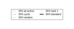
(a)

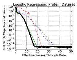
(b)

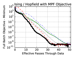
Figure C.1: SFO is insensitive to several specific design decisions. Plots showing the consequences of changing several of the design choices made in SFO for (a) the logistic regression objective, and (b) the Ising / Hopfield objective. SFO as described in this paper corresponds to the SFO standard line. All other lines correspond to changing a single design choice. SFO rank 1 corresponds to using a rank 1 rather than BFGS update (Section 2.4). SFO all active corresponds to starting optimization with all the subfunctions active (Section 3.4). SFO random and SFO cyclic correspond to random and cyclic update ordering, rather than maximum distance ordering (Section 3.3). For all design choices, SFO outperforms all other techniques in Figure 3.

Operation	One time cost	Repeats per pass	Cost per pass
Function and gradient computation	$\mathcal{O}\left(Q\right)$	$\mathcal{O}\left(N\right)$	$\mathcal{O}\left(QN\right)$
Subspace projection	$\mathcal{O}\left(MN\right)$	$\mathcal{O}\left(N\right)$	$\mathcal{O}\left(MN^{2}\right)$
Subspace collapse	$\mathcal{O}\left(MN^{1.4}+N^{3}\right)$	$\mathcal{O}\left(1\right)$	$\mathcal{O}\left(MN^{1.4}+N^{3}\right)$
Minimize $G^{t}\left(\mathbf{x}\right)$	$\leq\mathcal{O}\left(N^{2.4}\right)$	$\mathcal{O}\left(N\right)$	$\leq\mathcal{O}\left(N^{3.4}\right)$
BFGS	$\leq\mathcal{O}\left(NL^{2}+L^{3}\right)$	$\mathcal{O}\left(N\right)$	$\leq\mathcal{O}\left(N^{2}L^{2}+NL^{3}\right)$
Total			$\mathcal{O}\left(QN+MN^{2}+N^{3.4}+N^{2}L^{2}+NL^{3}\right)$

Table A.1: Computational cost for components of SFO. $Q$ is the cost of evaluating the objective function and gradient for a single subfunction, $M$ is the number of parameter dimensions, $N$ is the number of subfunctions, $L$ is the number of history terms kept per subfunction. Typically, $M\gg N\gg L$. In this case all contributions besides $\mathcal{O}\left(QN+MN^{2}\right)$ become small. Additionally the number of subfunctions can be chosen such that $\mathcal{O}\left(QN\right)=\mathcal{O}\left(MN^{2}\right)$ (see Section 4.1.1 in the main paper). Contributions labeled with ‘$\leq$’ could be reduced with small changes in implementation, as described in Section A. However as also discussed, and as illustrated by Figure 2 in the main text, they are not typically the leading terms in the cost of the algorithm.

References

- Amari (1998) Amari, Shun-Ichi. Natural Gradient Works Efficiently in Learning. Neural Computation, 10(2):251–276, 1998. ISSN 08997667. doi: 10.1162/089976698300017746.
- Bach & Moulines (2013) Bach, F and Moulines, E. Non-strongly-convex smooth stochastic approximation with convergence rate O (1/n). Neural Information Processing Systems, 2013.
- Bach & Moulines (2011) Bach, FR and Moulines, E. Non-Asymptotic Analysis of Stochastic Approximation Algorithms for Machine Learning. Neural Information Processing Systems, 2011.
- Bell & Sejnowski (1995) Bell, AJ and Sejnowski, TJ. An information-maximization approach to blind separation and blind deconvolution. Neural computation, 1995.
- Bergstra & Breuleux (2010) Bergstra, J and Breuleux, O. Theano: a CPU and GPU math expression compiler. Proceedings of the Python for Scientific Computing Conference (SciPy), 2010.
- Blatt et al. (2007) Blatt, Doron, Hero, Alfred O, and Gauchman, Hillel. A convergent incremental gradient method with a constant step size. SIAM Journal on Optimization, 18(1):29–51, 2007.
- Bordes et al. (2009) Bordes, Antoine, Bottou, Léon, and Gallinari, Patrick. SGD-QN: Careful quasi-Newton stochastic gradient descent. The Journal of Machine Learning Research, 10:1737–1754, 2009.
- Bottou (1991) Bottou, Léon. Stochastic gradient learning in neural networks. Proceedings of Neuro-Nimes, 91:8, 1991.
- Boyd & Vandenberghe (2004) Boyd, S P and Vandenberghe, L. Convex optimization. Cambridge Univ Press, 2004. ISBN 0521833787.
- Broyden (1970) Broyden, CG. The convergence of a class of double-rank minimization algorithms 2. The new algorithm. IMA Journal of Applied Mathematics, 1970.
- Byrd et al. (2014) Byrd, RH, Hansen, SL, Nocedal, J, and Singer, Y. A Stochastic Quasi-Newton Method for Large-Scale Optimization. arXiv preprint arXiv:1401.7020, 2014.
- Byrd et al. (2011) Byrd, RH Richard H, Chin, GM Gillian M, Neveitt, Will, and Nocedal, Jorge. On the use of stochastic hessian information in optimization methods for machine learning. SIAM Journal on Optimization, 21(3):977–995, 2011.
- Dennis Jr & Moré (1977) Dennis Jr, John E and Moré, Jorge J. Quasi-Newton methods, motivation and theory. SIAM review, 19(1):46–89, 1977.
- Duchi et al. (2010) Duchi, John, Hazan, Elad, and Singer, Yoram. Adaptive subgradient methods for online learning and stochastic optimization. Journal of Machine Learning Research, 12:2121–2159, 2010.
- Fletcher (1970) Fletcher, R. A new approach to variable metric algorithms. The computer journal, 1970.
- Goldfarb (1970) Goldfarb, D. A family of variable-metric methods derived by variational means. Mathematics of computation, 1970.
- Goodfellow & Warde-Farley (2013a) Goodfellow, IJ and Warde-Farley, D. Maxout networks. arXiv:1302.4389, 2013a.
- Goodfellow & Warde-Farley (2013b) Goodfellow, IJ and Warde-Farley, D. Pylearn2: a machine learning research library. arXiv:1308.4214, 2013b.
- Hennig (2013) Hennig, P. Fast probabilistic optimization from noisy gradients. International Conference on Machine Learning, 2013.
- Hillar et al. (2012) Hillar, Christopher, Sohl-Dickstein, Jascha, and Koepsell, Kilian. Efficient and optimal binary Hopfield associative memory storage using minimum probability flow. arXiv, 1204.2916, April 2012.
- Hinton et al. (2012) Hinton, Geoffrey E., Srivastava, Nitish, Krizhevsky, Alex, Sutskever, Ilya, and Salakhutdinov, Ruslan R. Improving neural networks by preventing co-adaptation of feature detectors. arXiv:1207.0580, 2012.
- Huber (1981) Huber, PJ. Robust statistics. Wiley, New York, 1981.
- Le et al. (2011) Le, Quoc V., Ngiam, Jiquan, Coates, Adam, Lahiri, Abhik, Prochnow, Bobby, and Ng, Andrew Y. On optimization methods for deep learning. International Conference on Machine Learning, 2011.
- Lin et al. (2008) Lin, Chih-Jen, Weng, Ruby C, and Keerthi, S Sathiya. Trust region newton method for logistic regression. The Journal of Machine Learning Research, 9:627–650, 2008.
- Liu & Nocedal (1989) Liu, Dong C DC and Nocedal, Jorge. On the limited memory BFGS method for large scale optimization. Mathematical programming, 45(1-3):503–528, 1989.
- Mairal (2013) Mairal, J. Optimization with First-Order Surrogate Functions. International Conference on Machine Learning, 2013.
- Mairal (2014) Mairal, Julien. Incremental Majorization-Minimization Optimization with Application to Large-Scale Machine Learning. arXiv:1402.4419, February 2014.
- Martens (2010) Martens, James. Deep learning via Hessian-free optimization. In Proceedings of the 27th International Conference on Machine Learning (ICML), volume 951, pp. 2010, 2010.
- Papakonstantinou (2009) Papakonstantinou, JM. Historical Development of the BFGS Secant Method and Its Characterization Properties. 2009.
- Pascanu et al. (2012) Pascanu, Razvan, Mikolov, Tomas, and Bengio, Yoshua. On the difficulty of training Recurrent Neural Networks. arXiv preprint arXiv:1211.5063., November 2012.
- Rifai et al. (2011) Rifai, Salah, Vincent, Pascal, Muller, Xavier, Glorot, Xavier, and Bengio, Yoshua. Contractive auto-encoders: Explicit invariance during feature extraction. In Proceedings of the 28th International Conference on Machine Learning (ICML-11), pp. 833–840, 2011.
- Robbins & Monro (1951) Robbins, Herbert and Monro, Sutton. A stochastic approximation method. The Annals of Mathematical Statistics, pp. 400–407, 1951.
- Roux et al. (2012) Roux, N Le, Schmidt, M, and Bach, F. A Stochastic Gradient Method with an Exponential Convergence Rate for Finite Training Sets. NIPS, 2012.
- Schraudolph et al. (2007) Schraudolph, Nicol, Yu, Jin, and Günter, Simon. A stochastic quasi-Newton method for online convex optimization. AIstats, 2007.
- Schraudolph (1999) Schraudolph, Nicol N. Local gain adaptation in stochastic gradient descent. In Artificial Neural Networks, 1999. ICANN 99. Ninth International Conference on (Conf. Publ. No. 470), volume 2, pp. 569–574. IET, 1999.
- Shanno (1970) Shanno, DF. Conditioning of quasi-Newton methods for function minimization. Mathematics of computation, 1970.
- Sohl-Dickstein (2012) Sohl-Dickstein, Jascha. The Natural Gradient by Analogy to Signal Whitening, and Recipes and Tricks for its Use. arXiv:1205.1828v1, May 2012.
- Sohl-Dickstein et al. (2011a) Sohl-Dickstein, Jascha, Battaglino, Peter, and DeWeese, Michael. New Method for Parameter Estimation in Probabilistic Models: Minimum Probability Flow. Physical Review Letters, 107(22):11–14, November 2011a. ISSN 0031-9007. doi: 10.1103/PhysRevLett.107.220601.
- Sohl-Dickstein et al. (2011b) Sohl-Dickstein, Jascha, Battaglino, Peter B., and DeWeese, Michael R. Minimum Probability Flow Learning. International Conference on Machine Learning, 107(22):11–14, November 2011b. ISSN 0031-9007. doi: 10.1103/PhysRevLett.107.220601.
- Sunehag et al. (2009) Sunehag, Peter, Trumpf, Jochen, Vishwanathan, S V N, and Schraudolph, Nicol. Variable metric stochastic approximation theory. arXiv preprint arXiv:0908.3529, August 2009.
- Vinyals & Povey (2011) Vinyals, Oriol and Povey, Daniel. Krylov subspace descent for deep learning. arXiv preprint arXiv:1111.4259, 2011.