An Experimental Comparison of Trust Region and Level Sets

Abstract

High-order (non-linear) functionals have become very popular in segmentation, stereo and other computer vision problems. Level sets is a well established general gradient descent framework, which is directly applicable to optimization of such functionals and widely used in practice. Recently, another general optimization approach based on trust region methodology was proposed for regional non-linear functionals [13]. Our goal is a comprehensive experimental comparison of these two frameworks in regard to practical efficiency, robustness to parameters, and optimality. We experiment on a wide range of problems with non-linear constraints on segment volume, appearance and shape.

1 Introduction

We study a general class of complex non-linear segmentation energies with high-order regional terms. Such energies are often desirable in the computer vision tasks of image segmentation, co-segmentation and stereo [15, 12, 22, 3, 2, 16, 14, 13] and are particularly useful when there is a prior knowledge about the appearance or the shape of an object being segmented.

We focus on energies of the following form:

$$\min_{S\in\Omega}E(S)=R(S)+\lambda L(S),$$ (1)

where $S$ is a binary segmentation, $L(S)$ is a standard length-based smoothness term, and $R(S)$ is a (generally) non-linear regional functional discussed below.

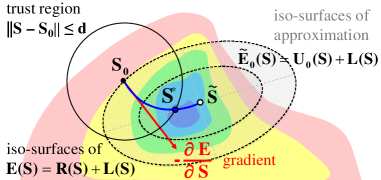
Figure 1: Gradient descent (level sets) and trust region.

Let $I:\Omega\to\mathbb{R}^{m}$ be an image defined in $\Omega\subset\mathbb{R}^{n}$. The most basic type of regional terms used in segmentation is a linear functional $U(S)$, which can be represented via an arbitrary scalar function $f:\Omega\to\mathbb{R}$

$$U(S)=\int_{S}f\,\text{d}x=\int_{\Omega}f\cdot 1_{S}\,\text{d}x=:\left\langle f,S\right\rangle.$$ (2)

Usually, $f$ corresponds to an appearance model based on image intensities/colors $I$, e.g., $f(x)$ could be a log-likelihood ratio for intensity $I(x)$ given particular object and background intensity distributions. The integral in (2) can be seen as a dot product between scalar function $f$ and $1_{S}$, which denotes the characteristic function of set $S$. We use notation $\left\langle f,S\right\rangle$ to refer to such linear functionals.

More general non-linear regional functional $R(S)$ can be described as follows. Assume $k$ scalar functions $f_{1},\ldots,f_{k}:\Omega\to\mathbb{R}$, each defining a linear functional $\left\langle f_{i},S\right\rangle$ of type (2), and one differentiable non-linear function $F(v_{1},\ldots,v_{k})\colon\mathbb{R}^{k}\to\mathbb{R}$ that combines them,

$$R(S)=F\left(\left\langle f_{1},S\right\rangle,\ldots,\left\langle f_{k},S\right\rangle\right).$$ (3)

Such general regional terms could enforce non-linear constraints on volume or higher-order shape moments of segment $S$. They could also penalize $L_{2}$ or other distance metrics between the distribution (or non-normalized bin counts) of intensities/colors inside segment $S$ and some given target. For example, $S$ could be softly constrained to specific volume $V_{0}$ via quadratic functional

$$R(S)=(\left\langle 1,S\right\rangle-V_{0})^{2}$$

using $f_{1}(x)=1$ and $F(v)=(v-V_{0})^{2}$, while the Kullback-Leibler (KL) divergence between the intensity distribution in $S$ and a fixed target distribution $q=(q_{1},\ldots,q_{k})$ could be written as

$$R(S)=\sum_{i}^{k}\frac{\left\langle f_{i},S\right\rangle}{\left\langle 1,S\right\rangle}\log\left(\frac{\left\langle f_{i},S\right\rangle}{\left\langle 1,S\right\rangle\cdot q_{i}}\right).$$

Here scalar function $f_{i}(x)$ is an indicator for pixels with intensity $i$ (in bin $i$). More examples of non-linear regional terms $R(S)$ are discussed in Section 3.

In general, optimization of non-linear regional terms is NP-hard and cannot be addressed by standard global optimization methods. Some earlier papers developed specialized techniques for particular forms of non-linear regional functionals. For example, the algorithm in [2] was developed for minimizing the Bhattacharyya distance between distributions and a dual-decomposition approach in [24] applies to convex piece-wise linear regional functionals (3). These methods are outside the scope of our paper since we focus on more general techniques. Combinatorial techniques [15, 22] apply to general non-linear regional functionals, and they can make large moves by globally minimizing some approximating energy. However, as pointed out in [14], these methods are known to converge to solutions that are not even a local minimum of energy (1). Level sets are a well established in the litterature as a gradient descent framework that can address arbitrary differentiable functionals [19], and therefore, are widely used for high-order terms [1, 11, 4, 18, 12].

This paper compares two known optimization methods applicable to energy (1) with any high-order regional term (3): trust region and level sets. To address non-linear term $R(S)$, both methods use its first-order functional derivative

$$\frac{\partial R}{\partial S}=\sum_{i=1}^{k}\frac{\partial F}{\partial v_{i}}\left(\left\langle f_{1},S\right\rangle,\ldots,\left\langle f_{k},S\right\rangle\right)\cdot f_{i}$$ (4)

either when computing gradient flow for (1) in level sets or when approximating energy (1) in trust region. However, despite using the same first derivative $\frac{\partial R}{\partial S}$, the level sets and trust region are fairly different approaches to optimize (1).

The structure of the paper is as follows. Sections 2.1-2.2 review the two general approaches that we compare: gradient descent implemented with level sets and trust region implemented with graph cuts. While the general trust region framework [13] can be based on a number of underlying global optimization techniques, we specifically choose a graph cut implementation (versus continuous convex relaxation approach), since it is more appropriate for our CPU-based evaluations. Our experimental results and comparisons are reported in Section 3 and Section 4 presents the conclusions.

2 Overview of Algorithms

Below we provide general background information on level sets and trust region methods, see Sections 2.1–2.2. High-level conceptual comparison of the two frameworks is provided in Section 2.3.

2.1 Standard Level Sets

In the level set framework, minimization of energy $E$ is carried out by computing a partial differential equation (PDE), which governs the evolution of the boundary of $S$. To this end, we derive the Euler-Lagrange equation by embedding segment $S$ in a one-parameter family $S(t)$, $t\in\mathbb{R}^{+}$, and solving a PDE of the general form:

$$\frac{\partial S}{\partial t}=-\frac{\partial E(S)}{\partial S}=-\frac{\partial R(S)}{\partial S}-\frac{\partial L(S)}{\partial S}$$ (5)

where $t$ is an artificial time step parameterizing the descent direction. The basic idea is to describe segment $S$ implicitly via an embedding function $\phi:\Omega\rightarrow\mathbb{R}$:

$$S = \{x\in\Omega|\phi(x)\leq 0\}$$

$$\Omega\setminus S = \{x\in\Omega|\phi(x)>0\},$$ (6)

and evolve $\phi$ instead of $S$. With the above representation, the terms that appear in energy (1) can be expressed as functions of $\phi$ as follows [9, 19]:

$$L(S) = \int_{\Omega}\|\nabla H(\phi)\|dx=\int_{\Omega}\delta(\phi)\|\nabla\phi\|dx$$

$$\left\langle f_{i},S\right\rangle = \int_{\Omega}H(\phi)f_{i}dx.$$ (7)

Here, $\delta$ and $H$ denote the Dirac function and Heaviside function, respectively. Therefore, the evolution equation in (5) can be computed directly by applying the Euler-Lagrange descent equation with respect to $\phi$. This gives the following gradient flow:

$$\frac{\partial\phi}{\partial t}=\left[-\frac{\partial R(S)}{\partial S}+\lambda\kappa\right]\delta(\phi)$$ (8)

with $\kappa:=\operatorname{div}\left(\frac{\nabla\phi}{\left\|\nabla\phi\right\|}\right)$ denoting the curvature of $\phi$’s level lines. The first term in (8) is a regional flow minimizing $R$, and the second is a standard curvature flow minimizing the length of the segment’s boundary.

In standard level set implementations, it is numerically mandatory to keep the evolving $\phi$ close to a distance function [17, 20]. This can be done by re-initialization procedures [20], which were intensively used in classical level set methods [8]. Such procedures, however, rely on several ad hoc choices and may result in undesirable side effects [17]. In our implementation, we use an efficient and well-known alternative [17], which adds an internal energy term that penalizes the deviation of $\phi$ from a distance function:

$$\frac{\mu}{2}\int_{\Omega}\left(1-\|\nabla\phi\|\right)^{2}dx.$$ (9)

In comparison to re-initialization procedures, the implementation in [17] allows larger time steps (and therefore faster curve evolution). Furthermore, it can be implemented via simple finite difference schemes, unlike traditional level set implementations which require complex upwind schemes [23]. With the distance-function penalty, the gradient flow in (8) becomes:

$$\frac{\partial\phi}{\partial t}=\mu\left[\Delta\phi-\kappa\right]+\left[-\frac{\partial R(S)}{\partial S}+\lambda\kappa\right]\delta(\phi)$$ (10)

For all the experiments in this paper, we implemented the flow in (10) using the numerical prescriptions in [17]. For each point $p$ of the discrete grid, we update the level set function as

$$\phi^{j+1}(p)=\phi^{j}(p)+\Delta t\cdot A(\phi^{j}(p)),$$ (11)

where $\Delta t$ is the discrete time step and $j$ is the iteration number. $A(\phi^{j}(p))$ is a numerical approximation of the right-hand side of (10), where the spatial derivatives of $\phi$ are approximated with central differences and the temporal derivative with forward differences. The Dirac function is approximated by $\delta_{\epsilon}(t)=\frac{1}{2\epsilon}[1+\cos(\frac{\pi t}{\epsilon})]$ for $|t|\leq\epsilon$ and $0$ elsewhere. We use $\epsilon=1.5$ and $\mu=0.05$.

In the context of level set and PDE methods, it is known that the choice of time steps should follow strict numerical conditions to ensure stability of front propagation, e.g., the standard Courant-Friedrichs-Lewy (CFL) conditions [10]. These conditions require that $\Delta t$ should be smaller than a certain value $\tau$ that depends on the choice of discretization. The level set literature generally uses fixed time steps. For instance, classical upwind schemes [23] generally require a small $\Delta t$ for stability, whereas the scheme in [17] allows relatively larger time steps. The optimum time step is not known a priori and finding a good $\Delta t<\tau$ via an adaptive search such as back-tracking [5] seems attractive. However, to apply a back-tracking scheme, we would have to evaluate the energy at each step. In the case of level sets, this requires a discrete approximation of the original continuous energy. We observed in our experiments that the gradient of such discrete approximation of the energy does not coincide with the gradient obtained in the numerical updates in  (11). Therefore, with a back-tracking scheme, level sets get stuck very quickly in a local minimum of the discrete approximation of the energy (See the adaptive level set example in Fig. 2). We believe that this is the main reason why, to the best of our knowledge, back-tracking approaches are generally avoided in the level-set literature. Therefore, in the following level-set experiments, we use a standard scheme based on fixed time step $\Delta t$ during each curve evolution, and report the performance at convergence for several values $\Delta t\in\{1\ldots 10^{3}\}$.

2.2 Trust Region Framework

Trust region methods are a class of iterative optimization algorithms. In each iteration, an approximate model of the optimization problem is constructed near the current solution. The model is only “trusted” within a small region around the current solution called “trust region”, since in general, approximations fit the original non-linear function only locally. The approximate model is then globally optimized within the trust region to obtain a candidate iterate solution. This step is often called trust region sub-problem. The size of the trust region is adjusted in each iteration based on the quality of the current approximation. Variants of trust region approach differ in the kind of approximate model used, optimizer for the trust region sub-problem step and a protocol to adjust the next trust region size. For a detailed review of trust region methods see [25].

Below we outline a general version of a trust region algorithm in the context of image segmentation. The goal is to minimize $E(S)$ in Eq. (1). Given solution $S_{j}$ and distance $d_{j}$, the energy $E$ is approximated using

$$\widetilde{E}(S)=U_{0}(S)+L(S),$$ (12)

where $U_{0}(S)$ is the first order Taylor approximation of the non-linear term $R(S)$ near $S_{j}$. The trust region sub-problem is then solved by minimizing $\widetilde{E}$ within the region given by $d_{j}$. Namely,

$$S^{*}=\underset{||S-S_{j}||<d}{\operatorname{argmin}}\tilde{E}(S).$$ (13)

Once a candidate solution $S^{*}$ is obtained, the quality of the approximation is measured using the ratio between the actual and predicted reduction in energy. The trust region is then adjusted accordingly.

For the purpose of our CPU-based evaluations we specifically selected the Fast Trust Region (FTR) implementation [13] which includes the following components for the trust region framework. The non-linear term $R(S)$ is approximated by the first order Taylor approximation $U_{0}(S)$ in (12) using first-order functional derivative (4). The trust region sub-problem in (13) is formulated as unconstrained Lagrangian optimization, which is globally optimized using one graph-cut (we use a floating point precision in the standard code for graph-cuts [7]). Note that, in this case, the length term $L(S)$ is approximated using Cauchy-Crofton formula as in [6]. More details about FTR can be found in [13].

2.3 Conceptual Comparison

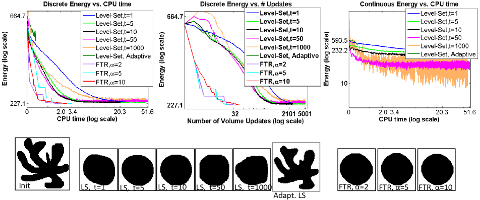
Figure 2: Volume constraint with boundary length regularization. We set the weights to $\lambda_{Length}=1$, $\lambda_{Volume}=10^{-4}$.

Some high-level conceptual differences between the level sets and trust region optimization frameworks are summarized in Figure 1. Standard level sets methods use fixed $\Delta t$ to make steps $-\Delta t\cdot\frac{\partial E}{\partial S}$ in the gradient descent direction. Trust region algorithm [13] moves to solution $S^{*}$ minimizing approximating functional $\tilde{E}(S)$ within a circle of given size $d$. The trust region size is adaptively changed from iteration to iteration based on the observed approximation quality. The blue line illustrates the spectrum of trust region moves for all values of $d$. Solution $\tilde{S}$ is the global minimum of approximation $\tilde{E}(S)$. For example, if $\tilde{E}(S)$ is a 2nd-order Taylor approximation of $E(S)$ at point $S_{0}$ then $\tilde{S}$ would correspond to a Newton’s step.

3 Experimental Comparison

In this section, we compare trust region and level sets frameworks in terms of practical efficiency, robustness and optimality. We selected several examples of segmentation energies with non-linear regional constraints. These include: 1) quadratic volume constraint, 2) shape prior in the form of $L_{2}$ distance between the target and the observed shape moments and 3) appearance prior in the form of either $L_{2}$ distance, Kullback-Leibler divergence or Bhattacharyya distance between the target and the observed color distributions.

In all the experiments below, we optimize energy of a general form $E(S)=R(S)+L(S)$. To compare optimization quality, we will plot energy values for the results of both level sets and trust region. Note that the Fast Trust Region (FTR) implementation uses a discrete formulation based on graph-cuts and level sets are a continuous framework. Thus, the direct comparison of their corresponding energy values should be done carefully. While numerical evaluation of the regional term $R(S)$ is equivalent in both methods, they use completely different numerical approaches to measuring length $L(S)$. In particular, level sets use the approximation of length given in (2.1), while the graph cut variant of trust region relies on integral geometry and Cauchy-Crofton formula popularized by [6].

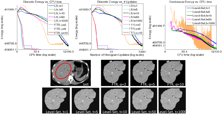
Figure 3: Shape prior constraint with length regularization and log-likelihood models. Target shape moments and appearance models are computed from the provided ellipse. We used 100 intensity bins, moments up to order $l=2$, $\lambda_{Length}=10$, $\lambda_{Shape}=0.01$ and $\lambda_{App}=1$. The continuous energy is plotted starting from $4^{th}$ iteration to reduce the range of the y-axis.

Since the energies are not comparable by its actual number, we study instead the robustness of each method independently and compare the resulting segmentation with one another. Note that level sets have much smaller oscillation for small time steps, which supports the theory of the CFL-conditions.

In each application below we examine the robustness of both trust region and level sets methods by varying the running parameters. In the trust region method we vary the multiplier $\alpha$ used to change the size of the trust region from one iteration to another. For the rest of the parameters we follow the recommendations of [13]. In our implementation of level sets we vary the time-step size $\Delta t$, but keep the parameters $\epsilon=1.5$ and $\mu=0.05$ fixed for all the experiments.

The top-left plots in figures 2-6 report energy $E(S)$ as a function of the CPU time. At the end of each iteration, both level sets and trust region require energy updates, which could be computationally expensive. For example, appearance-based regional functionals require re-evaluation of color histograms/distributions at each iteration. This is a time consuming step. Therefore, for completeness of our comparison, we report in the top-middle plots of each figure energy $E(S)$ versus the number of energy evaluations (number of updates) required during the optimization.

3.1 Volume Constraint

First, we perform image segmentation with a volume constraint with respect to a target volume $V_{0}$, namely,

$$R(S)=(\left\langle 1,S\right\rangle-V_{0})^{2}.$$

We choose to optimize this energy on a synthetic image without appearance term since the solution to this problem is known to be a circle. Figure 2 shows that both FTR and level sets converge to good solutions (nearly circle), with FTR being 25 times faster, requiring 150 times less energy updates and exhibiting more robustness to the parameters.

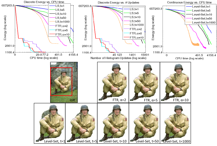
Figure 4: $L_{2}$ norm between the observed and target color bin counts with length regularization. We used 100 bins per channel, $\lambda_{App}=1$ and $\lambda_{Length}=1$.

3.2 Shape Prior with Geometric Shape Moments

Next, we perform image segmentation with a shape prior constraint in the form of $L_{2}$ distance between the geometric shape moments of the segment and a target. Our energy is defined as $E(S)=\lambda_{Shape}R(S)+\lambda_{Length}L(S)+\lambda_{App}D(S)$, where $D(S)$ is a standard log-likelihood unary term based on intensity histograms. In this case, $R(S)$ is given by

$$R(S)=\sum_{p+q\leq l}(\left\langle x^{p}y^{q},S\right\rangle-m_{pq})^{2},$$

with $m_{pq}$ denoting the target geometric moment of order $l=p+q$. Figure 3 shows an example of liver segmentation with the above shape prior constraint. The target shape moments as well as the foreground and background appearance models are computed from the user provided input ellipse as in [16, 13]. We used moments of up to order $l=2$ (including the center of mass and shape covariance but excluding the volume). Both trust region and level sets obtain visually pleasing solutions. The trust region method is two orders of magnitude faster and requires two orders of magnitude less energy updates (top-left and top-middle plots). Since the level sets method was forced to stop after 10000 iterations, we show the last solution available for each value of parameter $\Delta t$ . The actual convergence for this method would have taken more iterations. In this example, the oscillations of the energy are especially pronounced (top-right plot).

3.3 Appearance Prior

In the experiments below, we apply both methods to optimize segmentation energies where the goal is to match a given target appearance distribution using either the $L_{2}$ distance between the observed and target color bin counts, or the Kullback-Leibler divergence and Bhattacharyya distance between the observed and target color distributions. Here, our energy is defined as $E(S)=\lambda_{App}R(S)+\lambda_{Length}L(S)$. We assume $f_{i}$ is an indicator function of pixels belonging to bin $i$ and $q_{i}$ is the target count (or probability) for bin $i$. The target appearance distributions for the object and the background were obtained from the ground truth segments. We used 100 bins per color channel. The images in the experiments below are taken from [21].

$L_{2}$ distance constraint on bin counts:

Figure 4 shows results of segmentation with $L_{2}$ distance constraint between the observed and target bin counts regularized by length. The regional term in this case is

$$R(S)=\sqrt{\sum_{i=1}^{k}(\left\langle f_{i},S\right\rangle-q_{i})^{2}}.$$

Since the level sets method was forced to stop after 15000 iterations for values of $\Delta t=1,5$, we show the last solution available. Full convergence would have taken more iterations. For higher values of $\Delta t$, we show results at convergence. We observe two orders of magnitude difference between the trust region and level sets method in terms of the speed and the number of energy updates required.

Kullback-Leibler divergence:

Figure 5 shows results of segmentation with KL divergence constraint between the observed and target color distributions. The regional term in this case is given by

$$R(S)=\sum_{i=1}^{k}\frac{\left\langle f_{i},S\right\rangle}{\left\langle 1,S\right\rangle}\log\left(\frac{\left\langle f_{i},S\right\rangle}{\left\langle 1,S\right\rangle q_{i}}\right).$$

The level sets method converged for times steps $\Delta t=50$ and $1000$ , but was forced to stop for other values of the parameter after $10000$ iterations. We show the last solution available. Full convergence would have required more iterations. The trust region method obtains solutions that are closer to the ground truth, runs two order of magnitude faster and requires less energy updates.

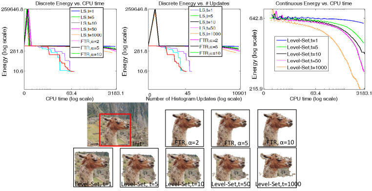
Figure 5: KL divergence between the observed and the target color distribution. We used 100 bins per channel, $\lambda_{App}=100$ and $\lambda_{Length}=0.01$. Continuous energy is plotted starting from forth iteration to reduce the range of the y-axis.

Bhattacharyya divergence:

Figure 6 shows results of segmentation with Bhattacharyya distance constraint between the observed and target color distributions. The regional term in this case is given by

$$R(S)=-\log\left(\sum_{i=1}^{k}\sqrt{\frac{\left\langle f_{i},S\right\rangle}{\left\langle 1,S\right\rangle}q_{i}}\right).$$

Also for this image, since the level sets method had not (yet) converged after 10000 iterations for any set of the parameters, we show the last solution available. Further increasing parameter $\Delta t$ would increase the oscillations of the energy (see top-right plot).

4 Conclusions

For relatively simple functionals (3), combining a few linear terms ($k$ is small), such as constraints on volume and low-order shape moments, the quality of the results obtained by both methods is comparable (visually and energy-wise). However, we observe that the number of energy updates required for level sets is two orders of magnitude larger than for trust region. This behavior is consistent with the corresponding CPU running time plots. The segmentation results on shape moments were fairly robust with respect to parameters (time step $\Delta t$ and multiplier $\alpha$) for both methods. The level sets results for volume constraints varied with the choice of $\Delta t$. In general, larger steps caused significant oscillations of the energy in level sets thereby affecting the quality of the result at convergence.

When optimizing appearance-based regional functionals with large number of histogram bins (corresponding to large $k$), level sets proved to be extremely slow. Convergence would require more than $10^{4}$ iterations (longer than 1 hour on our machine). In some cases, the corresponding results were far from optimal both visually and energy-wise. This is in contrast to the results by trust region approach, which consistently converged to plausible solutions with low energy in less than a minute or $100$ iterations.

We believe that our results will be useful for many practitioners in computer vision and medical imaging when selecting an optimization technique.

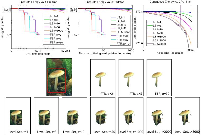
Figure 6: Bhattacharyya distance between the observed and the target color distribution. We used 100 bins per channel, $\lambda_{App}=1000$ and $\lambda_{Length}=0.01$.

References

- [1] A. Adam, R. Kimmel, and E. Rivlin. On scene segmentation and histograms-based curve evolution. IEEE Transactions on Pattern Analysis and Machine Intelligence (TPAMI), 31:1708–1714, 2009.
- [2] I. Ben Ayed, H. Chen, K. Punithakumar, I. Ross, and S. Li. Graph cut segmentation with a global constraint: Recovering region distribution via a bound of the Bhattacharyya measure. In IEEE Conf. on Computer Vision and Pattern Recognition (CVPR), pages 3288 – 3295, 2010.
- [3] I. Ben Ayed, S. Li, A. Islam, G. Garvin, , and R. Chhem. Area prior constrained level set evolution for medical image segmentation. In Proc. SPIE, Medical Imaging 2008: Image Processing, 2008.
- [4] I. Ben Ayed, S. Li, and I. Ross. A statistical overlap prior for variational image segmentation. International Journal of Computer Vision, 85(1):115–132, 2009.
- [5] S. Boyd and L. Vandenberghe. Convex Optimization. Cambridge University Press, 2004.
- [6] Y. Boykov and V. Kolmogorov. Computing Geodesics and Minimal Surfaces via Graph Cuts. In IEEE Int. Conf. on Computer Vision (ICCV), 2003.
- [7] Y. Boykov and V. Kolmogorov. An Experimental Comparison of Min-Cut/Max-Flow Algorithms for Energy Minimization in Vision. IEEE Transactions on Pattern Analysis and Machine Intelligence (TPAMI), 29(9):1124–1137, 2004.
- [8] V. Caselles, R. Kimmel, and G. Sapiro. Geodesic active contours. International Journal of Computer Vision, 22(1):61–79, 1997.
- [9] T. Chan and L. Vese. Active contours without edges. IEEE Transactions on Image Processing (TIP), 10(2):266–277, 2001.
- [10] V. Estellers, D. Zosso, R. Lai, S. Osher, J. P. Thiran, and X. Bresson. Efficient algorithm for level set method preserving distance function. IEEE Transactions on Image Processing (TIP), 21(12):4722–34, 2012.
- [11] A. Foulonneau, P. Charbonnier, and F. Heitz. Multi-reference shape priors for active contours. International Journal of Computer Vision, 81(1):68–81, 2009.
- [12] D. Freedman and T. Zhang. Active contours for tracking distributions. IEEE Transactions on Image Processing (TIP), 13:518 – 526, April 2004.
- [13] L. Gorelick, F. Schmidt, and Y. Boykov. Fast Trust Region for Segmentation. In IEEE Conf. on Computer Vision and Pattern Recognition (CVPR), June 2013.
- [14] L. Gorelick, R. Schmidt, Y. Boykov, A. Delong, and A. Ward. Segmentation with Non-Linear Regional Constraint via Line-Search cuts. In European Conf. on Computer Vision (ECCV), 2012.
- [15] J. Kim, V. Kolmogorov, and R. Zabih. Visual correspondence using energy minimization and mutual information. In IEEE Int. Conf. on Computer Vision (ICCV), pages 1033 – 1040, 2003.
- [16] M. Klodt and D. Cremers. A convex framework for image segmentation with moment constraints. In IEEE Int. Conf. on Computer Vision (ICCV), 2011.
- [17] C. Li, C. Xu, C. Gui, and M. D. Fox. Level set evolution without re-initialization: A new variational formulation. In IEEE Conf. on Computer Vision and Pattern Recognition (CVPR), pages 430–436, 2005.
- [18] O. V. Michailovich, Y. Rathi, and A. Tannenbaum. Image segmentation using active contours driven by the bhattacharyya gradient flow. IEEE Transactions on Image Processing (TIP), 16(11):2787–2801, 2007.
- [19] A. Mitiche and I. Ben Ayed. Variational and Level Set Methods in Image Segmentation. Springer, 2011.
- [20] S. Osher and R. Fedkiw. Level Set Methods and Dynamic Implicit Surfaces. Springer-Verlag, 2002.
- [21] C. Rother, V. Kolmogorov, and A. Blake. GrabCut: Interactive Foreground Extraction using Iterated Graph Cuts. In ACM SIGGRAPH, 2004.
- [22] C. Rother, V. Kolmogorov, T. Minka, and A. Blake. Cosegmentation of Image Pairs by Histogram Matching - Incorporating a Global Constraint into MRFs. In IEEE Conf. on Computer Vision and Pattern Recognition (CVPR), pages 993 – 1000, 2006.
- [23] J. A. Sethian. Level set Methods and Fast Marching Methods. Cambridge University Press, 1999.
- [24] O. J. Woodford, C. Rother, and V. Kolmogorov. A global perspective on MAP inference for low-level vision. In IEEE Int. Conf. on Computer Vision (ICCV), pages 2319 – 2326, 2009.
- [25] Y. Yuan. A review of trust region algorithms for optimization. In International Congress on Industrial and Applied Mathematics, 1999.