Querying Knowledge Graphs by Example Entity Tuples

Abstract

We witness an unprecedented proliferation of knowledge graphs that record millions of entities and their relationships. While knowledge graphs are structure-flexible and content-rich, they are difficult to use. The challenge lies in the gap between their overwhelming complexity and the limited database knowledge of non-professional users. If writing structured queries over “simple” tables is difficult, complex graphs are only harder to query. As an initial step toward improving the usability of knowledge graphs, we propose to query such data by example entity tuples, without requiring users to form complex graph queries. Our system, $\mathsf{GQBE}$ (Graph Query By Example), automatically derives a weighted hidden maximal query graph based on input query tuples, to capture a user’s query intent. It efficiently finds and ranks the top approximate answer tuples. For fast query processing, $\mathsf{GQBE}$ only partially evaluates query graphs. We conducted experiments and user studies on the large Freebase and DBpedia datasets and observed appealing accuracy and efficiency. Our system provides a complementary approach to the existing keyword-based methods, facilitating user-friendly graph querying. To the best of our knowledge, there was no such proposal in the past in the context of graphs.

I Introduction

There is an unprecedented proliferation of knowledge graphs that record millions of entities (e.g., persons, products, organizations) and their relationships. Fig.1 is an excerpt of a knowledge graph, in which the edge labeled founded between nodes Jerry Yang and Yahoo! captures the fact that the person is a founder of the company. Examples of real-world knowledge graphs include DBpedia [3], YAGO [25], Freebase [4] and Probase [31]. Users and developers are tapping into knowledge graphs for numerous applications, including search, recommendation and business intelligence.

Both users and application developers are often overwhelmed by the daunting task of understanding and using knowledge graphs. This largely has to do with the sheer size and complexity of such data. As of March 2012, the Linking Open Data community had interlinked over 52 billion RDF triples spanning over several hundred datasets. More specifically, the challenges lie in the gap between complex data and non-expert users. Knowledge graphs are often stored in relational databases, graph databases and triplestores (cf. [19] for a tutorial).

Figure 1: An Excerpt of a Knowledge Graph

Figure 2: Query Interface of $\mathsf{GQBE}$

In retrieving data from these databases, the norm is often to use structured query languages such as SQL, SPARQL, and those alike. However, writing structured queries requires extensive experiences in query language and data model and good understanding of particular datasets [12]. Graph data is not “easier” than relational data in either query language or data model. The fact it is schema-less makes it even more intangible to understand and query. If querying “simple” tables is difficult, aren’t complex graphs harder to query?

Figure 3: The Architecture and Components of $\mathsf{GQBE}$

Motivated by the aforementioned usability challenge, we build $\mathsf{GQBE}$  (Graph Query by Example), a system that queries knowledge graphs by example entity tuples instead of graph queries. Given a data graph and a query tuple consisting of entities, $\mathsf{GQBE}$ finds similar answer tuples. Consider the data graph in Fig.1 and an scenario where a Silicon Valley business analyst is interested in finding entrepreneurs who have founded technology companies head-quartered in California. Suppose she knows an example 2-entity query tuple such as $\langle\textsf{\scriptsize Jerry Yang},\textsf{\scriptsize Yahoo!}\rangle$ that satisfies her query intent. As the query interface in Fig. 2 shows, entering such an example tuple to $\mathsf{GQBE}$ is simple, especially with the help of user interface tools such as auto-completion in identifying the exact entities in the data graph. The answer tuples can be $\langle\textsf{\scriptsize Steve Wozniak},\textsf{\scriptsize Apple Inc.}\rangle$ and $\langle\textsf{\scriptsize Sergey Brin},\textsf{\scriptsize Google}\rangle$, which are founder-company pairs. If the query tuple consists of 3 or more entities (e.g., $\langle\textsf{\scriptsize Jerry Yang},\textsf{\scriptsize Yahoo!},$ $\textsf{\scriptsize Sunnyvale}\rangle$), the answers will be similar tuples of the same cardinality (e.g., $\langle\textsf{\scriptsize Steve Wozniak},\textsf{\scriptsize Apple Inc.},\textsf{\scriptsize Cupertino}\rangle$).

Our work is the first to query knowledge graphs by example entity tuples. The paradigm of query-by-example (QBE) has a long history in relational databases [35]. The idea is to express queries by filling example tables with constants and shared variables in multiple tables, which correspond to selection and join conditions, respectively. Its simplicity and improved user productivity make QBE an influential database query language. By proposing to query knowledge graphs by example tuples, our premise is that the QBE paradigm will enjoy similar advantages on graph data. The technical challenges and approaches are vastly different, due to the fundamentally different data models.

Substantial progress has been made on query mechanisms that help users construct query graphs or even do not require explicit query graphs. Such mechanisms include keyword search (e.g., [16]), keyword-based query formulation [24, 33], natural language questions [32], interactive and form-based query formulation [8, 13], and visual interface for query graph construction [6, 15]. Little has been done on comparison across these graph query mechanisms. While a usability comparison of these mechanisms and $\mathsf{GQBE}$ is beyond the scope of this paper, we note that they all have pros and cons and thus complement each other.

Particularly, QBE and keyword-based methods are adequate for different usage scenarios. Using keyword-based methods, a user has to articulate query keywords, e.g., “technology companies head-quartered in California and their founders” for the aforementioned analyst. Not only a user may find it challenging to clearly articulate a query, but also a query system might not return accurate answers, since it is non-trivial to precisely separate these keywords and correctly match them with entities, entity types and relationships. This has been verified through our own experience on a keyword-based system adapted from SPARK [22]. In contrast, a $\mathsf{GQBE}$ user only needs to know the names of some entities in example tuples, without being required to specify how exactly the entities are related. On the other hand, keyword-based querying is more adequate when a user does not know a few sample answers with respect to her query.

In the literature on graph query, the input to a query system in most cases is a structured query, which is often graphically presented as a query graph or pattern. Such is not what we refer to as query-by-example, because the query graphs and patterns are formed by using structured query languages or the aforementioned query mechanisms. For instance, $\mathsf{PathSim}$ [26] finds the top-k similar entities that are connected to a query entity, based on a user-defined meta-path semantics in a heterogeneous network. In [34], given a query graph as input, the system finds structurally isomorphic answer graphs with semantically similar entity nodes. In contrast, $\mathsf{GQBE}$ only requires a user to provide an entity tuple, without knowing the underlying schema.

There are several challenges in building $\mathsf{GQBE}$. Below we provide a brief overview of our approach in tackling these challenges. The ensuing discussion refers to the system architecture and components of $\mathsf{GQBE}$, as shown in Fig. 3.

(1) With regard to query semantics, since the input to $\mathsf{GQBE}$ is a query tuple instead of an explicit query graph, the system must derive a hidden query graph based on the query tuple, to capture user’s query intent. The query graph discovery component (Sec.III) of $\mathsf{GQBE}$ fulfills this requirement and the derived graph is termed a maximal query graph (MQG). The edges in MQG, weighted by several frequency-based and distance-based heuristics, represent important “features” of the query tuple to be matched in answer tuples. More concretely, they capture how entities in the query tuple (i.e., nodes in a data graph) and their neighboring entities are related to each other. Answer graphs matching the MQG are projected to answer tuples, which consist of answer entities corresponding to the query tuple entities. $\mathsf{GQBE}$ further supports multiple query tuples as input which collectively better capture the user intent.

(2) With regard to answer space modeling (Sec.IV), there can be a large space of approximate answer graphs (tuples), since it is unlikely to find answer graphs exactly matching the MQG. $\mathsf{GQBE}$ models the space of answer tuples by a query lattice formed by the subsumption relation between all possible query graphs. Each query graph is a subgraph of the MQG and contains all query entities. Its answer graphs are also subgraphs of the data graph and are isomorphic to the query graph. Given an answer graph, its entities corresponding to the query tuple entities form an answer tuple. Thus the answer tuples are essentially approximate answers to the MQG. For ranking answer tuples, their scores are calculated based on the edge weights in their query graphs and the match between nodes in the query and answer graphs.

(3) The query lattice can be large. To obtain top-k ranked answer tuples, the brute-force approach of evaluating all query graphs in the lattice can be prohibitively expensive. For efficient query processing (Sec.V), $\mathsf{GQBE}$ employs a top-$k$ lattice exploration algorithm that only partially evaluates the lattice nodes in the order of their corresponding query graphs’ upper-bound scores.

We summarize the contributions of this paper as follows:

• For better usability of knowledge graph querying systems, we propose a novel approach of querying by example entity tuples, which saves users the burden of forming explicit query graphs. To the best of our knowledge, there was no such proposal in the past.

• The query graph discovery component of $\mathsf{GQBE}$ derives a hidden maximal query graph (MQG) based on input query tuples, to capture users’ query intent. $\mathsf{GQBE}$ models the space of query graphs (and thus answer tuples) by a query lattice based on the MQG.

• $\mathsf{GQBE}$’s efficient query processing algorithm only partially evaluates the query lattice to obtain the top-k answer tuples ranked by how well they approximately match the MQG.

• We conducted extensive experiments and user study on the large Freebase and DBpedia datasets to evaluate $\mathsf{GQBE}$’s accuracy and efficiency (Sec.VI). The comparison with a state-of-the-art graph querying framework $\mathsf{NESS}$ [18] (using MQG as input) shows that $\mathsf{GQBE}$ is twice as accurate as $\mathsf{NESS}$ and outperforms $\mathsf{NESS}$ on efficiency in most of the queries.

II Problem Formulation

$\mathsf{GQBE}$ runs queries on knowledge data graphs. A data graph is a directed multi-graph $G$ with node set $V(G)$ and edge set $E(G)$. Each node $v$$\in$$V(G)$ represents an entity and has a unique identifier $id(v)$.  Each edge $e$=$(v_{i},v_{j})$$\in$$E(G)$ denotes a directed relationship from entity $v_{i}$ to entity $v_{j}$. It has a label, denoted as $label(e)$. Multiple edges can have the same label. The user input and output of $\mathsf{GQBE}$ are both entity tuples, called query tuples and answer tuples, respectively. A tuple $t$=$\langle v_{1},\ldots,v_{n}\rangle$ is an ordered list of entities (i.e., nodes) in $G$. The constituting entities of query (answer) tuples are called query (answer) entities. Given a data graph $G$ and a query tuple $t$, our goal is to find the top-k answer tuples $t^{\prime}$ with the highest similarity scores $\textsf{score}_{t}(t^{\prime})$.

Figure 4: Neighborhood Graph for $\langle\textsf{\scriptsize Jerry Yang},\textsf{\scriptsize Yahoo!}\rangle$

Figure 5: Two Query Graphs in Fig.4

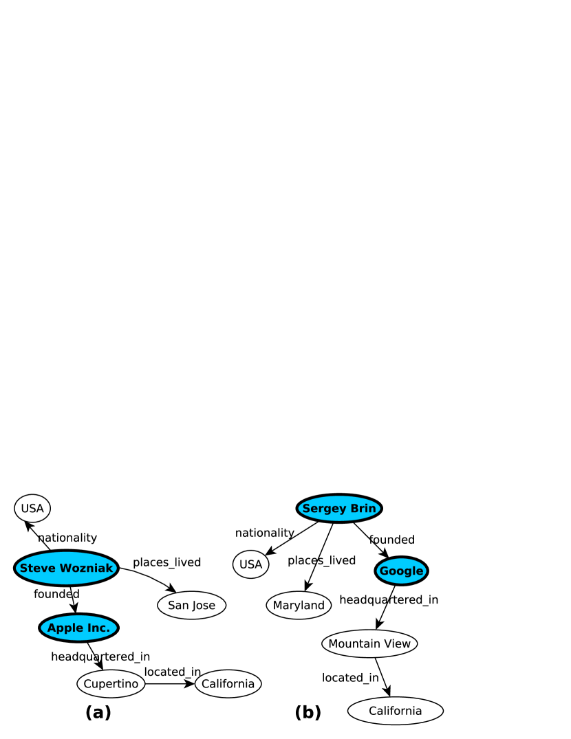
Figure 6: Two Answer Graphs for Fig.7(a)

Figure 7: Two Answer Graphs for Fig.7(b)

We define $\textsf{score}_{t}(t^{\prime})$ by matching the inter-entity relationships of $t$ and that of $t^{\prime}$, which entails matching two graphs constructed from $t$ and $t^{\prime}$, respectively. To this end, we define the neighborhood graph for a tuple, which is based on the concept of undirected path. An undirected path is a path whose edges are not necessarily oriented in the same direction. Unless otherwise stated, we will refer to undirected path simply as “path”. We consider undirected path because an edge incident on a node can represent an important relationship with another node, regardless of its direction. More formally, a path $p$ is a sequence of edges $e_{1},\ldots,e_{n}$ and we say each edge $e_{i}\in p$. The path connects two nodes $v_{0}$ and $v_{n}$ through intermediate nodes $v_{1},\ldots,v_{n-1}$, where either $e_{i}$=$(v_{i-1},v_{i})$ or $e_{i}$=$(v_{i},v_{i-1})$, for all $1$$\leq$$i$$\leq$$n$. The length of the path, $len(p)$, is $n$ and the endpoints of the path, $ends(p)$, are $\{v_{0},v_{n}\}$. Note that there is no undirected cycle in a path, i.e., the entities $v_{0},\ldots,v_{n}$ are all distinct.

Definition 1.

The neighborhood graph of query tuple $t$, denoted $H_{t}$, is the weakly connected subgraph of data graph $G$ that consists of all nodes reachable from at least one query entity by an undirected path of $d$ or less edges (including query entities themselves) and the edges on all such paths. The path length threshold, $d$, is an input parameter. More formally, the nodes and edges in $H_{t}$ are defined as follows:

$V(H_{t})=\{v\lvert v\in V(G)$ and $\exists p$ s.t. $ends(p)$=$\{v_{i},v\}$ where $v_{i}\in t\text{, }len(p)\leq d\}$;

$E(H_{t})=\{e\lvert e\in E(G)$ and $\exists p$ s.t. $ends(p)$=$\{v_{i},v\}$ where $v_{i}\in t,len(p)\leq d$, and $e\in p\}$.

Example 1 (Neighborhood Graph).

Given the data graph in Fig.1, Fig.4 shows the neighborhood graph for query tuple $\langle\textsf{\scriptsize Jerry Yang},\textsf{\scriptsize Yahoo!}\rangle$ with path length threshold $d$=2. The nodes in dark color are the query entities.

Intuitively, the neighborhood graph, by capturing how query entities and other entities in their neighborhood are related to each other, represents “features” of the query tuple that are to be matched in query answers. It can thus be viewed as a hidden query graph derived for capturing user’s query intent. We are unlikely to find query answers that exactly match the neighborhood graph. It is however possible to find exact matches to its subgraphs. Such subgraphs are all query graphs and their exact matches are approximate answers that match the neighborhood graph to different extents.

Definition 2.

A query graph $Q$ is a weakly connected subgraph of $H_{t}$ that contains all the query entities. We use $\mathcal{Q}_{t}$ to denote the set of all query graphs for $t$, i.e., $\mathcal{Q}_{t}$={$Q|Q$ is a weakly connected subgraph of $H_{t}$ s.t. $\forall v\in t$, $v\in V(Q)$}.

Continuing the running example, Fig.7 shows two query graphs for the neighborhood graph in Fig.4.

Echoing the intuition behind neighborhood graph, the definitions of answer graph and answer tuple are based on the idea that an answer tuple is similar to the query tuple if their entities participate in similar relationships in their neighborhoods.

Definition 3.

An answer graph $A$ to a query graph $Q$ is a weakly connected subgraph of $G$ that is isomorphic to $Q$. Formally, there exists a bijection $f$$:$$V(Q)$$\rightarrow$$V(A)$ such that:

• For every edge $e=(v_{i},v_{j})\in E(Q)$, there exists an edge $e^{\prime}=(f(v_{i}),f(v_{j}))\in E(A)$ such that $label(e)=label(e^{\prime})$;

• For every edge $e^{\prime}=(u_{i},u_{j})\in E(A)$, there exists $e=(f^{-1}(u_{i}),f^{-1}(u_{j}))\in E(Q)$ such that $label(e)=label(e^{\prime})$.

For a query tuple $t$=$\langle v_{1},\ldots,v_{n}\rangle$, the answer tuple in $A$ is $t_{A}$=$\langle f(v_{1}),\ldots,f(v_{n})\rangle$. We also call $t_{A}$ the projection of $A$.

We use $\mathcal{A}_{Q}$ to denote the set of all answer graphs of $Q$. We note that a query graph (tuple) trivially matches itself, therefore is not considered an answer graph (tuple).

Example 2 (Answer Graph and Answer Tuple).

Fig.7 and Fig.7 each show two answer graphs for query graphs Fig.7(a) and Fig.7(b), respectively. The answer tuples in Fig.7 are $\langle\textsf{\scriptsize Steve Wozniak}$, $\textsf{\scriptsize Apple Inc.}\rangle$ and $\langle\textsf{\scriptsize Sergey Brin},\textsf{\scriptsize Google}\rangle$. The answer tuples in Fig.7 are $\langle\textsf{\scriptsize Bill Gates},\textsf{\scriptsize Microsoft}\rangle$ and $\langle\textsf{\scriptsize Sergey Brin},\textsf{\scriptsize Google}\rangle$.

Definition 4.

The set of answer tuples for query tuple $t$ are $\{t_{A}|A$$\in$$\mathcal{A}_{Q},Q$$\in$$\mathcal{Q}_{t}\}$. The score of an answer $t^{\prime}$ is given by

$$\textsf{score}_{t}(t^{\prime})=\max_{A\in\mathcal{A}_{Q},Q\in\mathcal{Q}_{t}}\{{\textsf{score}_{Q}}(A)|t^{\prime}=t_{A}\}$$ (1)

The score of an answer graph $A$ (${\textsf{score}_{Q}}(A)$) captures $A$’s similarity to query graph $Q$. Its equation is given in Sec.IV-B.

The same answer tuple $t^{\prime}$ may be projected from multiple answer graphs, which can match different query graphs. For instance, Figs. 7(b) and 7(b), which are answers to different query graphs, have the same projection—$\langle\textsf{\scriptsize Sergey Brin}$, $\textsf{\scriptsize Google}\rangle$. By Eq. (1), the highest score attained by the answer graphs is assigned as the score of $t^{\prime}$, capturing how well $t^{\prime}$ matches $t$.

III Query Graph Discovery

III-A Maximal Query Graph

The concept of neighborhood graph $H_{t}$ (Def.1) was formed to capture the features of a query tuple $t$ to be matched by answer tuples. Given a well-connected large data graph, $H_{t}$ itself can be quite large, even under a small path length threshold $d$. For example, using Freebase as the data graph, the query tuple $\langle\textsf{\scriptsize Jerry Yang},\textsf{\scriptsize Yahoo!}\rangle$ produces a neighborhood graph with $800$K nodes and $900$K edges, for $d$=$2$. Such a large $H_{t}$ makes query semantics obscure, because there might be only few nodes and edges in it that capture important relationships in the neighborhood of $t$.

$\mathsf{GQBE}$’s query graph discovery component constructs a weighted maximal query graph (MQG) from the neighborhood graph $H_{t}$. MQG is expected to be drastically smaller than $H_{t}$ and capture only important features of the query tuple. We now define MQG and discuss its discovery algorithm.

Definition 5.

The maximal query graph $MQG_{t}$, given a parameter $m$, is a weakly connected subgraph of the neighborhood graph $H_{t}$ that maximizes total edge weight $\sum_{e}\textsf{w}(e)$ while satisfying (1) it contains all query entities in $t$ and (2) it has $m$ edges. The weight of an edge $e$ in $H_{t}$, $\textsf{w}(e)$, is defined in Sec.III-B.

There are two challenges in finding $MQG_{t}$ by directly going after the above definition. First, a weakly connected subgraph of $H_{t}$ with exactly $m$ edges may not exist for an arbitrary $m$. A trivial value of $m$ that guarantees the existence of the corresponding $MQG_{t}$ is $|E(H_{t})|$, because $H_{t}$ itself is weakly connected. This value could be too large, which is exactly why we aim to make $MQG_{t}$ substantially smaller than $H_{t}$. Second, even if $MQG_{t}$ exists for an $m$, finding it requires maximizing the total edge weight, which is a hard problem as given in Theorem 1.

Theorem 1.

The decision version of finding the maximal query graph $MQG_{t}$ for an $m$ is NP-hard.

Proof.

We prove the NP-hardness by reduction from the NP-hard constrained Steiner network (CSN) problem [20]. Given an undirected connected graph $G_{1}$=$(V,E)$ with non-negative weight $w(e)$ for every $e$$\in$$E$, a subset $V_{n}$$\subset$$V$, and a positive integer $m$, the CSN problem is to find a connected subgraph $G^{\prime}$=$(V^{\prime},E^{\prime})$ with the smallest total edge weight, where $V_{n}$$\subseteq$$V^{\prime}$ and $|E^{\prime}|$=$m$. The polynomial-time reduction from the CSN problem to the MQG problem is by transforming $G_{1}$ to $G_{2}$, where each edge $e$ is given an arbitrary direction and a new weight $w^{\prime}(e)$=$W$$-$$w(e)$, where $W$=$\sum_{e\in E}w(e)$. Let $V_{n}$ be the query tuple. The maximal query graph $MQG_{V_{n}}$ found from $G_{2}$ provides a CSN in $G_{1}$, by ignoring edge direction. This completes the proof.

Input: neighborhood graph $H_{t}$, query tuple $t$, an integer $r$

1

Output: maximal query graph $MQG_{t}$

2

3$m\leftarrow\frac{r}{\lvert t\lvert+1}$; $V(MQG_{t})\leftarrow\phi$; $E(MQG_{t})\leftarrow\phi$; $\mathcal{G}\leftarrow\phi$;

4foreach $v_{i}\in t$ do

5       $G_{v_{i}}\leftarrow$ use DFS to obtain the subgraph containing vertices (and their incident edges) that connect to other $v_{j}$ in $t$ only through $v_{i}$;

6       $\mathcal{G}\leftarrow\mathcal{G}\cup\{G_{v_{i}}\}$;

7      

8 $G_{core}\leftarrow$ use DFS to obtain the subgraph containing vertices and edges on undirected paths between query entities;

9 $\mathcal{G}\leftarrow\mathcal{G}\cup\{G_{core}\}$;

10 foreach $G\in\mathcal{G}$ do

11       $step\leftarrow 1$; $s_{1}\leftarrow 0$; $s\leftarrow m$;

12      while $s>0$ do

13             $M_{s}\leftarrow$ the weakly connected component found from the top-$s$ edges of $G$ that contains all of $G$’s query entities;

14            if $M_{s}$ exists then

15                   if $|E(M_{s})|=m$ then break;

16                  

17                  if $|E(M_{s})|<m$ then

18                         $s_{1}\leftarrow s$;

19                        if $step=-1$ then break;

20                        

21                  if $|E(M_{s})|>m$ then

22                         if $s_{1}>0$ then

23                               $s\leftarrow s_{1}$; break;

24                        $s_{2}\leftarrow s$; $step\leftarrow-1$;

25                  

26            $s\leftarrow s+step$;

27      

28      if $s=0$ then $s\leftarrow s_{2}$;

29      

30      $V(MQG_{t})\leftarrow V(MQG_{t})\cup V(M_{s})$;

31       $E(MQG_{t})\leftarrow E(MQG_{t})\cup E(M_{s})$;

32      

Algorithm 1 Discovering the Maximal Query Graph

Based on the theoretical analysis, we present a greedy method (Alg.1) to find a plausible sub-optimal graph of edge cardinality close to a given $m$. The value of $m$ is empirically chosen to be much smaller than $|E(H_{t})|$. Consider edges of $H_{t}$ in descending order of weight $\textsf{w}(e)$. We use $G_{s}$ to denote the graph formed by the top $s$ edges with the largest weights, which itself may not be weakly connected. We use $M_{s}$ to denote the weakly connected component of $G_{s}$ containing all query entities in $t$, if it exists. Our method finds the smallest $s$ such that $|E(M_{s})|$=$m$ (Line 1). If such an $M_{s}$ does not exist, the method chooses $s_{1}$, the largest $s$ such that $|E(M_{s})|$$<$$m$. If that still does not exist, it chooses $s_{2}$, the smallest $s$ such that $|E(M_{s})|$$>$$m$, whose existence is guaranteed because $|E(H_{t})|$$>$$m$. For each $s$ value, the method employs a depth-first search (DFS) starting from a query entity in $G_{s}$, if present, to check the existence of $M_{s}$ (Line 1).

The $M_{s}$ found by this method may be unbalanced. Query entities with more neighbors in $H_{t}$ likely have more prominent representation in the resulting $M_{s}$. A balanced graph should instead have a fair number of edges associated with each query entity. Therefore, we further propose a divide-and-conquer mechanism to construct a balanced $MQG_{t}$. The idea is to break $H_{t}$ into $n$$+$$1$ weakly connected subgraphs. One is the core graph, which includes all the $n$ query entities in $t$ and all undirected paths between query entities. Other $n$ subgraphs are for the $n$ query entities individually, where the subgraph for entity $v_{i}$ includes all entities (and their incident edges) that connect to other query entities only through $v_{i}$. The subgraphs are identified by a DFS starting from each query entity (Lines 1-1 of Alg.1). During the DFS from $v_{i}$, all edges on the undirected paths reaching any other query entity within distance $d$ belong to the core graph, and other edges belong to $v_{i}$’s individual subgraph. The method then applies the aforementioned greedy algorithm to find $n$$+$$1$ weakly connected components, one for each subgraph, that contain the query entities in corresponding subgraphs. Since the core graph connects all query entities, the $n$$+$$1$ components altogether form a weakly connected subgraph of $H_{t}$, which becomes the final $MQG_{t}$. For an empirically chosen small $r$ as the target size of $MQG_{t}$, we set the target size for each individual component to be $\frac{r}{n+1}$, aiming at a balanced $MQG_{t}$.

Complexity Analysis of Alg.1   In the aforementioned divide-and-conquer method, if on average there are $r^{\prime}$=$\frac{\lvert E(H_{t})\lvert}{n+1}$ edges in each subgraph, finding the subgraph by DFS and sorting its $r^{\prime}$ edges takes $O(r^{\prime}\log r^{\prime})$ time. Given the top-$s$ edges of a subgraph, checking if the weakly connected component $M_{s}$ exists using DFS requires $O(s)$ time. Suppose on average $c$ iterations are required to find the appropriate $s$. Let $m$=$\frac{r}{n+1}$ be the average target edge cardinality of each subgraph. Since the method initializes $s$ with $m$, the largest value $s$ can attain is $m$$+$$c$. So the time for discovering $M_{s}$ for each subgraph is $O(r^{\prime}\log r^{\prime}$$+$$c$$\times$$(m$$+$$c$)). For all $n$$+$$1$ subgraphs, the total time required to find the final $MQG_{t}$ is $O((n$$+$$1)\times(r^{\prime}\log r^{\prime}$$+$$c$$\times$$(m$$+$$c)))$. For the queries used in our experiments on Freebase, given an empirically chosen small $r$=$15$, $s$$\ll$$\lvert E(H_{t})\lvert$ and on average $c$=$22$.

III-B Edge Weighting

The definition of $MQG_{t}$ (Def.5) depends on edge weights. There can be various plausible weighting schemes. We propose a weighting function based on several heuristic ideas. The weight of an edge $e$ in $H_{t}$, $\textsf{w}(e)$, is proportional to its inverse edge label frequency ($\textsf{ief}(e)$) and inversely proportional to its participation degree ($\textsf{p}(e)$), given by

$$\textsf{w}(e)=\textsf{ief}(e)\;/\;\textsf{p}(e)$$ (2)

Inverse Edge Label Frequency   Edge labels that appear frequently in the entire data graph $G$ are often less important. For example, edges labeled founded (for a company’s founders) can be rare and more important than edges labeled nationality (for a person’s nationality). We capture this by the inverse edge label frequency.

$$\textsf{ief}(e)=\log\;(|E(G)|\;/\;\#label(e))$$ (3)

where $|E(G)|$ is the number of edges in $G$, and $\#label(e)$ is the number of edges in $G$ with the same label as $e$.

Participation Degree   The participation degree $p(e)$ of an edge $e$=$(u,v)$ is the number of edges in $G$ that share the same label and one of $e$’s end nodes. Formally,

$$\textsf{p}(e)=\lvert\ \{e^{\prime}\textrm{=}(u^{\prime},v^{\prime})\ |\ label(e)\textrm{=}label(e^{\prime}),u^{\prime}\textrm{=}u\vee v^{\prime}\textrm{=}v\}\ \lvert$$ (4)

While $\textsf{ief}(e)$ captures the global frequencies of edge labels, $\textsf{p}(e)$ measures their local frequencies—an edge is less important if there are other edges incident on the same node with the same label. For instance, employment might be a relatively rare edge globally but not necessarily locally to a company. Specifically, consider the edges representing the employment relationship between a company and its many employees and the edges for the board member relationship between the company and its few board members. The latter edges are more significant.

Note that $\textsf{ief}(e)$ and $\textsf{p}(e)$ are precomputed offline, since they are query-independent and only rely on the data graph $G$.

III-C Preprocessing: Reduced Neighborhood Graph

The discussion so far focuses on discovering $MQG_{t}$ from $H_{t}$. The neighborhood graph $H_{t}$ may have clearly unimportant edges. As a preprocessing step, $\mathsf{GQBE}$ removes such edges from $H_{t}$ before applying Alg.1. The reduced size of $H_{t}$ not only makes the execution of Alg.1 more efficient but also helps prevent clearly unimportant edges from getting into $MQG_{t}$.

Consider the neighborhood graph $H_{t}$ in Fig.4, based on the data graph excerpt in Fig.1. Edge $e_{1}$=(Jerry Yang, Stanford) and $label$($e_{1}$)=education. Two other edges labeled education, $e_{2}$ and $e_{3}$, are also incident on node Stanford. The neighborhood graph from a complete real-world data graph may contain many such edges for people graduated from Stanford University. Among these edges, $e_{1}$ represents an important relationship between Stanford and query entity Jerry Yang, while other edges represent relationships between Stanford and other entities, which are deemed unimportant with respect to the query tuple.

We formalize the definition of unimportant edges as follows. Given an edge $e$=$(u,v)\in E(H_{t})$, $e$ is unimportant if it is unimportant from the perspective of its either end, $u$ or $v$, i.e., $\text{if }e\in UE(u)\ \text{or}\ e\in UE(v)$. Given a node $v\in V(H_{t})$, $E(v)$ denotes the edges incident on $v$ in $H_{t}$. $E(v)$ is partitioned into three disjoint subsets—the important edges $IE(v)$, the unimportant edges $UE(v)$ and the rest—defined as follows:

$IE(v)$=

$\{e\in E(v)\ \lvert\ \exists v_{i}$$\in$$t,p\text{ s.t. }e$$\in$$p,ends(p)$=$\{v,v_{i}\},len(p)$$\leq$$d\}$;

$UE(v)$=

$\{e\in E(v)\ \lvert\ e$$\notin$$IE(v),\exists e^{\prime}$$\in$$IE(v)\text{ s.t. }label(e)$=$label(e^{\prime})$,

$(e$=$(u,v)\wedge e^{\prime}$=$(u^{\prime},v))\vee(e$=$(v,u)\wedge e^{\prime}$=$(v,u^{\prime}))\}$.
An edge $e$ incident on $v$ belongs to $IE(v)$ if there exists a path between $v$ and any query entity in the query tuple $t$, through $e$, with path length at most $d$. For example, edge $e_{1}$ in Fig.4 belongs to $IE(\textsf{\scriptsize Stanford})$. An edge $e$ belongs to $UE(v)$ if (1) it does not belong to $IE(v)$ (i.e., there exists no such aforementioned path) and (2) there exists $e^{\prime}\in IE(v)$ such that $e$ and $e^{\prime}$ have the same label and they are both either incoming into or outgoing from $v$. By this definition, $e_{2}$ and $e_{3}$ belong to $UE(v)$ in Fig.4, since $e_{1}$ belongs to $IE(v)$. In the same neighborhood graph, $e_{4}$ is in neither $IE(v)$ nor $UE(v)$.

All edges deemed unimportant by the above definition are removed from $H_{t}$. The resulting graph may not be weakly connected anymore and may have multiple weakly connected components.  Theorem 2 states that one of the components—called the reduced neighborhood graph, denoted $H^{\prime}_{t}$—contains all query entities in $t$. In other words, $H^{\prime}_{t}$ is the largest weakly connected subgraph of $H_{t}$ containing all query entities and no unimportant edges. Alg.1 is applied on $H^{\prime}_{t}$ (instead of $H_{t}$) to produce $MQG_{t}$. Since the techniques in the ensuing discussion only operate on $MQG_{t}$, the distinction between $H_{t}$ and $H^{\prime}_{t}$ will not be further noted.

Theorem 2.

Given the neighborhood graph $H_{t}$ for a query tuple $t$, the reduced neighborhood graph $H^{\prime}_{t}$ always exists.

Proof.

We prove by contradiction. Suppose that, after removal of all unimportant edges, $H_{t}$ becomes a disconnected graph, of which none of the weakly connected components contains all the query entities. The deletion of unimportant edges must have disconnected at least a pair of query entities, say, $v_{i}$ and $v_{j}$. By Def. 1, before removal of unimportant edges, $H_{t}$ must have at least a path $p$ of length at most $d$ between $v_{i}$ and $v_{j}$. By the definition of unimportant edges, every edge $e$=$(u,v)$ on $p$ belongs to both $IE(u)$ and $IE(v)$ and thus cannot be an unimportant edge. However, the fact that $v_{i}$ and $v_{j}$ become disconnected implies that $p$ consists of at least one unimportant edge which is deleted. This presents a contradiction and completes the proof.

III-D Multi-tuple Queries

The query graph discovery component of $\mathsf{GQBE}$ essentially derives a user’s query intent from input query tuples. For that, a single query tuple might not be sufficient. While the experiment results in Sec.VI show that a single-tuple query obtains excellent accuracy in many cases, the results also exhibit that allowing multiple query tuples often helps improve query answer accuracy. This is because important relationships commonly associated with multiple query tuples express the user intent more precisely. For instance, suppose a user has provided two query tuples together—$\langle\textsf{\scriptsize Jerry Yang},\textsf{\scriptsize Yahoo!}\rangle$ and $\langle\textsf{\scriptsize Steve Wozniak},\textsf{\scriptsize Apple Inc.}\rangle$. The query entities in both tuples share common properties such as places_lived in San Jose and headquartered_in a city in California, as shown in Fig.1. This might indicate that the user is interested in finding people from San Jose who founded technology companies in California.

Given a set of tuples $T$, $\mathsf{GQBE}$ aims at finding top-$k$ answer tuples similar to $T$ collectively. To accomplish this, one approach is to discover and evaluate the maximal query graphs (MQGs) of individual query tuples. The scores of a common answer tuple for multiple query tuples can then be aggregated. This has two potential drawbacks: (1) Our concern of not being able to well capture user intent still remains. If $k$ is not large enough, a good answer tuple may not appear in enough individual top-$k$ answer lists, resulting in poor aggregated score. (2) It can become expensive to evaluate multiple MQGs.

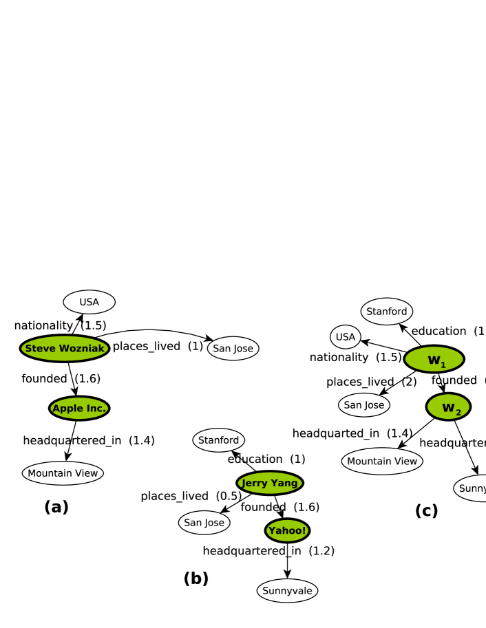
Figure 8: Merging Maximal Query Graphs

We approach this problem by producing a merged and re-weighted MQG that captures the importance of edges with respect to their presence across multiple MQGs. The merged MQG is then processed by the same method for single-tuple queries. $\mathsf{GQBE}$ employs a simple strategy to merge multiple MQGs. The individual MQG for a query tuple $t_{i}$=$\langle v_{1}^{i},v_{2}^{i},\ldots,v_{n}^{i}\rangle$$\in$$T$ is denoted $M_{t_{i}}$. A virtual MQG $M_{t_{i}}^{\prime}$ is created for every $M_{t_{i}}$ by replacing the query entities $v_{1}^{i},v_{2}^{i},\ldots,v_{n}^{i}$ in $M_{t_{i}}$ with corresponding virtual entities $w_{1},w_{2},\ldots,w_{n}$ in $M_{t_{i}}^{\prime}$. Formally, there exists a bijective function $g$$:$$V(M_{t_{i}})$$\rightarrow$$V(M_{t_{i}}^{\prime})$ such that (1) $g(v_{j}^{i})$=$w_{j}$ and $g(v)$=$v$ if $v$$\notin$$t_{i}$, and (2) $\forall e$=$(u,v)$$\in$$E(M_{t_{i}})$, there exists an edge $e^{\prime}$=$(g(u),g(v))$ $\in$$E(M_{t_{i}}^{\prime})$ such that $label(e)$=$label(e^{\prime})$; $\forall e^{\prime}$=$(u^{\prime},v^{\prime})$$\in$$E(M_{t_{i}}^{\prime})$, $\exists$$e$ =$(g^{-1}(u^{\prime}),g^{-1}(v^{\prime}))$$\in$$E(M_{t_{i}})$ such that $label(e)$=$label(e^{\prime})$.

The merged MQG is denoted $MQG_{T}$. It is produced by including vertices and edges in all $M_{t_{i}}^{\prime}$, merging identical virtual and regular vertices, and merging identical edges that bear the same label and the same vertices on both ends. Formally,

$$\textstyle V(MQG_{T})=\bigcup\limits_{t_{i}\in T}V(M_{t_{i}}^{\prime})\text{ and }E(MQG_{T})=\bigcup\limits_{t_{i}\in T}E(M_{t_{i}}^{\prime}).$$

The edge cardinality of $MQG_{T}$ might be larger than the target size $r$. Thus Alg.1 proposed in Sec.III-A is also used to trim $MQG_{T}$ to a size close to $r$. In $MQG_{T}$, the weight of an edge $e$ is given by $c*\textsf{w}_{max}(e)$, where $c$ is the number of $M_{t_{i}}^{\prime}$ containing $e$ and $\textsf{w}_{max}(e)$ is its maximal weight among all such $M_{t_{i}}^{\prime}$.

Example 3 (Merging Maximal Query Graphs).

Let Figs. 8 (a) and (b) be the $M_{t_{i}}$ for query tuples $\langle\textsf{\scriptsize Steve Wozniak},\textsf{\scriptsize Apple Inc.}\rangle$ and $\langle\textsf{\scriptsize Jerry Yang},\textsf{\scriptsize Yahoo!}\rangle$, respectively. Fig.8(c) is the merged $MQG_{T}$. Note that entities Steve Wozniak and Jerry Yang are mapped to $w_{1}$ in their respective $M_{t_{i}}^{\prime}$ (not shown, for its mapping from $M_{t_{i}}$ is simple) and are merged into $w_{1}$ in $MQG_{T}$. Similarly, entities Apple Inc. and Yahoo! are mapped and merged into $w_{2}$. The two founded edges, appearing in both individual $M_{t_{i}}$ and sharing identical vertices on both ends ($w_{1}$ and $w_{2}$) in the corresponding $M_{t_{i}}^{\prime}$, are merged in $MQG_{T}$. Similarly the two places_lived edges are merged. However, the two headquartered_in edges are not merged, since they share only one end ($w_{2}$) in $M_{t_{i}}^{\prime}$. The edges nationality and education, which appear in only one $M_{t_{i}}$, are also present in $MQG_{T}$. The number next to each edge is its weight.

In comparison to evaluating a single-tuple query, the extra overhead in handling a multi-tuple query includes creating multiple MQGs, which is $\lvert T\lvert$ times the average cost of discovering an individual MQG, and merging them, which is linear in the total edge cardinality of all MQGs.

IV Answer Space Modeling

Given the maximal query graph $MQG_{t}$ for a tuple $t$, we model the space of possible query graphs by a lattice. We further discuss the scoring of answer graphs by how well they match query graphs.

IV-A Query Lattice

Definition 6.

The query lattice $\mathcal{L}$ is a partially ordered set (poset) ($\mathcal{QG}_{t}$, $\prec$), where $\prec$ represents the subgraph-supergraph subsumption relation and $\mathcal{QG}_{t}$ is the subset of query graphs (Def.2) that are subgraphs of $MQG_{t}$, i.e., $\mathcal{QG}_{t}$$=$$\{Q|Q\in\mathcal{Q}_{t}\text{ and }Q\preceq MQG_{t}\}$. The top element (root) of the poset is thus $MQG_{t}$. When represented by a Hasse diagram, the poset is a directed acyclic graph, in which each node corresponds to a distinct query graph in $\mathcal{QG}_{t}$. Thus we shall use the terms lattice node and query graph interchangeably. The children (parents) of a lattice node $Q$ are its subgraphs (supergraphs) with one less (more) edge, as defined below.

$$\textsf{Children}(Q)=\{Q^{\prime}|Q^{\prime}\in\mathcal{QG}_{t},Q^{\prime}\prec Q,|E(Q)|\!-\!|E(Q^{\prime})|\!=\!1\}$$

$$\textsf{Parents}(Q)=\{Q^{\prime}|Q^{\prime}\in\mathcal{QG}_{t},Q\prec Q^{\prime},|E(Q^{\prime})|\!-\!|E(Q)|\!=\!1\}$$

The leaf nodes of $\mathcal{L}$ constitute of the minimal query trees, which are those query graphs that cannot be made any simpler and yet still keep all the query entities connected.

Definition 7.

A query graph $Q$ is a minimal query tree if none of its subgraphs is also a query graph. In other words, removing any edge from $Q$ will disqualify it from being a query graph—the resulting graph either is not weakly connected or does not contain all the query entities. Note that such a $Q$ must be a tree.

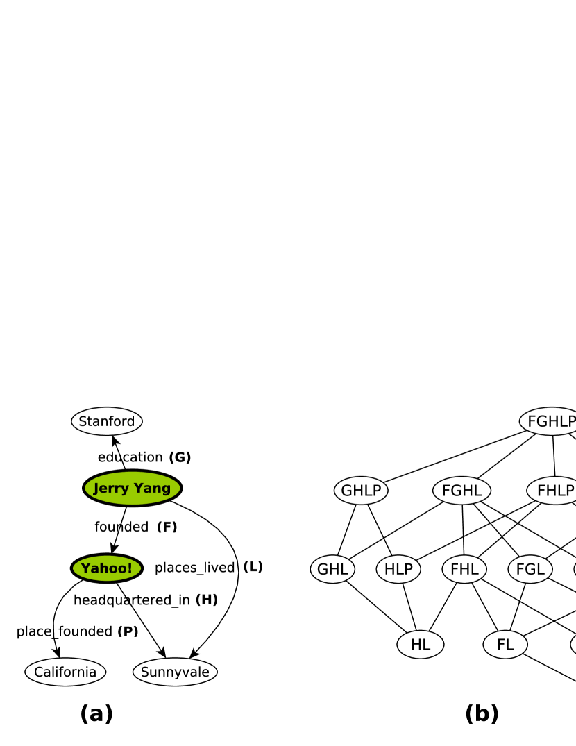
Figure 9: Maximal Query Graph and Query Lattice

Example 4 (Query Lattice and Minimal Query Tree).

Fig.9(a) shows a maximal query graph $MQG_{t}$, which contains two query entities in shaded circles and five edges $F,G,H,L,$ and $P$. Its corresponding query lattice $\mathcal{L}$ is in Fig.9(b). The root node of $\mathcal{L}$, denoted $FGHLP$, represents $MQG_{t}$ itself. The two bottom nodes, $F$ and $HL$, are the two minimal query trees. Each lattice node is a distinct subgraph of $MQG_{t}$. For example, the node $FLP$ represents a query graph with only edges $F,L$ and $P$. Note that there is no lattice node for $GLP$, which is not a valid query graph since it is not connected.

The construction of the query lattice, i.e., the generation of query graphs corresponding to its nodes, is integrated with its exploration. In other words, the lattice is built in a “lazy” manner—a lattice node is not generated until the query algorithm (Sec.V) must evaluate it. The lattice nodes are generated in a bottom-up way. A node is generated by adding exactly one appropriate edge to the query graph for one of its children. The generation of bottom nodes, i.e., the minimal query trees, is described below.

By definition, a minimal query tree can only contain edges on undirected paths between query entities. Hence, it must be a subgraph of the weakly connected component $M_{s}$ found from the core graph described in Sec.III-A. To generate all minimal query trees, our method enumerates all distinct spanning trees of $M_{s}$ by the technique in [10] and then trim them. Specifically, given one such spanning tree, all non-query entities (nodes) of degree one along with their edges are deleted. The deletion is performed iteratively until there is no such node. The result is a minimal query tree. Only distinct minimal query trees are kept. Enumerating all spanning trees in a large graph is expensive. However, in our experiments on the Freebase dataset, the $MQG_{t}$ discovered by the approach in Sec.III mostly contains less than $15$ edges. Hence, the $M_{s}$ from the core graph is also empirically small, for which the cost of enumerating all spanning trees is negligible.

IV-B Answer Graph Scoring Function

The score of an answer graph $A$ (${\textsf{score}_{Q}}(A)$) captures $A$’s similarity to the query graph $Q$. It is defined below and is to be plugged into Eq. (1) for defining answer tuple score.

$$\begin{aligned} {\textsf{score}_{Q}}(A)&={\textsf{s\_score}}(Q)+{\textsf{c\_score}_{Q}}(A)\\ {\textsf{s\_score}}(Q)&=\;\;\;\;\;\sum_{e\in E(Q)}{\textsf{w}(e)}\\ {\textsf{c\_score}_{Q}}(A)&=\!\!\!\!\!\!\sum_{\begin{subarray}{c}e=(u,v)\in E(Q)\\ e^{\prime}=(f(u),f(v))\in E(A)\end{subarray}}\!\!\!\!\!\!\!\!\!\!\!\!\textsf{match}(e,e^{\prime})\end{aligned}$$ (5)

In Eq. (5), ${\textsf{score}_{Q}}(A)$ sums up two components—the structure score of $Q$ (${\textsf{s\_score}}(Q)$) and the content score for $A$ matching $Q$ (${\textsf{c\_score}_{Q}}(A)$). ${\textsf{s\_score}}(Q)$ is the total edge weight of $Q$. It measures the important structure in $MQG_{t}$ that is captured by $Q$ and thus by $A$. ${\textsf{c\_score}_{Q}}(A)$ is the total extra credit for identical nodes among the matching nodes in $A$ and $Q$ given by $f$—the bijection between $V(Q)$ and $V(A)$ as in Def.3. For instance, among the $6$ pairs of matching nodes between Fig.7(a) and Fig.7(a), the identical matching nodes are USA, San Jose and California. The rationale for the extra credit is that although node matching is not mandatory, the more nodes are matched, the more similar $A$ and $Q$ are.

The extra credit is defined by the following function $\textsf{match}(e,e^{\prime})$. Note that it does not award an identical matching node excessively. Instead, only a fraction of $\textsf{w}(e)$ is awarded, where the denominator is either $|E(u)|$ or $|E(v)|$. ($E(u)$ are the edges incident on $u$ in $MQG_{t}$.) This heuristic is based on that, when $u$ and $f(u)$ are identical, many of their neighbors can be also identical matching nodes.

$$\textsf{match}(e,e^{\prime})\text{=}\begin{cases}\frac{\textsf{w}(e)}{\lvert{E(u)}\lvert}&\text{if }u\text{=}f(u)\\ \frac{\textsf{w}(e)}{\lvert{E(v)}\lvert}&\text{if }v\text{=}f(v)\\ \frac{\textsf{w}(e)}{min(\lvert{E(u)}\lvert,\lvert{E(v)}\lvert)}&\text{if }u\text{=}f(u),v\text{=}f(v)\\ 0&\text{otherwise}\end{cases}$$ (6)

In discovering $MQG_{t}$ from $H_{t}$ by Alg.1, the weights of edges in $H_{t}$ are defined by Eq. (2) which does not consider an edge’s distance from the query tuple. The rationale behind the design is to obtain a balanced $MQG_{t}$ which includes not only edges incident on query entities but also those in the larger neighborhood. For scoring answers by Eq. (5) and Eq. (6), however, our empirical observations show it is imperative to differentiate the importance of edges in $MQG_{t}$ with respect to query entities, in order to capture how well an answer graph matches $MQG_{t}$. Edges closer to query entities convey more meaningful relationships than those farther away. Hence, we define edge depth ($\textsf{d}(e)$) as follows. The larger $\textsf{d}(e)$ is, the less important $e$ is.

Edge Depth   The depth $\textsf{d}(e)$ of an edge $e$=$(u,v)$ is its smallest distance to any query entity $v_{i}\in t$, i.e.,

$$\textsf{d}(e)=\min_{v_{i}\in t}\min_{u,v}\{\textsf{dist}(u,v_{i}),\textsf{dist}(v,v_{i})\}$$ (7)

Here, $\textsf{dist}(.,.)$ is the shortest length of all undirected paths in $MQG_{t}$ between the two nodes.

In summary, $\mathsf{GQBE}$ uses Eq. (2) as the definition of $\textsf{w}(e)$ in weighting edges in $H_{t}$. After $MQG_{t}$ is discovered from $H_{t}$ by Alg.1, it uses the following Eq. (8) as the definition of $\textsf{w}(e)$ in weighting edges in $MQG_{t}$. Eq. (8) incorporates $\textsf{d}(e)$ into Eq. (2). The answer graph scoring functions Eq. (5) and Eq. (6) are based on Eq. (8).

$$\textsf{w}(e)=\textsf{ief}(e)\;/\;(\textsf{p}(e)\times\textsf{d}^{2}(e))$$ (8)

V Query Processing

The query processing component of $\mathsf{GQBE}$ takes the maximal query graph $MQG_{t}$ (Sec.III) and the query lattice $\mathcal{L}$ (Sec.IV) and finds answer graphs matching the query graphs in $\mathcal{L}$. Before we discuss how $\mathcal{L}$ is evaluated (Sec.V-B), we introduce the storage model and query plan for processing one query graph (Sec.V-A).

V-A Processing One Query Graph

The abstract data model of knowledge graph can be represented by the Resource Description Framework (RDF)—the standard Semantic Web data model. In RDF, a data graph is parsed into a set of triples, each representing an edge $e$=$(u,v)$. A triple has the form (subject, property, object), corresponding to ($u,label(e),v$). Among different schemes of RDF data management, one important approach is to use relational database techniques to store and query RDF graphs. To store a data graph, we adopt this approach and, particularly, the vertical partitioning method [1]. This method partitions a data graph into multiple two-column tables. Each table is for a distinct edge label and stores all edges bearing that label. The two columns are ($subj,obj$), for the edges’ source and destination nodes, respectively. For efficient query processing, two in-memory search structures (specifically, hash tables) are created on the table, using $subj$ and $obj$ as the hash keys, respectively. The whole data graph is hashed in memory by this way, before any query comes in.

Given the above storage scheme, to evaluate a query graph is to process a multi-way join query. For instance, the query graph in Fig.9(a) corresponds to SELECT F.subj, F.obj FROM F,G,H,L,P WHERE F.subj=G.sbj AND F.obj=H.subj AND F.subj=L.subj AND F.obj=P.subj AND H.obj=L.obj. We use right-deep hash-joins to process such a query. Consider the topmost join operator in a join tree for query graph $Q$. Its left operand is the build relation which is one of the two in-memory hash tables for an edge $e$. Its right operand is the probe relation which is a hash table for another edge or a join subtree for $Q^{\prime}$=$Q$$-$$e$ (i.e., the resulting graph of removing $e$ from $Q$). For instance, one possible join tree for the aforementioned query is $G$$\bowtie$$(F$$\bowtie$$(P$$\bowtie$$(H$$\bowtie$$L)))$. With regard to its topmost join operator, the left operand is $G$’s hash table that uses $G.sbj$ as the hash key, and the right operand is $(F$$\bowtie$$(P$$\bowtie$$(H$$\bowtie$$L)))$. The hash-join operator iterates through tuples from the probe relation, finds matching tuples from the build relation, and joins them to form answer tuples.

V-B Best-first Exploration of Query Lattice

Given a query lattice, a brute-force approach is to evaluate all lattice nodes (query graphs) to find all answer tuples. Its exhaustive nature leads to clear inefficiency, since we only seek top-k answers. Moreover, the potentially many queries are evaluated separately, without sharing of computation. Suppose query graph $Q$ is evaluated by the aforementioned hash-join between the build relation for $e$ and the probe relation for $Q^{\prime}$. By definition, $Q^{\prime}$ is also a query graph in the lattice, if $Q^{\prime}$ is weakly connected and contains all query entities. In other words, in processing $Q$, we would have processed one of its children query graph $Q^{\prime}$ in the lattice.

We propose Alg.2, which allows sharing of computation. It explores the query lattice in a bottom-up way, starting with the minimal query trees, i.e., the bottom nodes. After a query graph is processed, its answers are materialized in files. To process a query $Q$, at least one of its children $Q^{\prime}$=$Q$$-$$e$ must have been processed. The materialized results for $Q^{\prime}$ form the probe relation and a hash table on $e$ is the build relation.

While any topological order would work for the bottom-up exploration, Alg.2 employs a best-first strategy that always chooses to evaluate the most promising lattice node $Q_{best}$ from a set of candidate nodes. The gist is to process the lattice nodes in the order of their upper-bound scores and $Q_{best}$ is the candidate with the highest upper-bound score (Line 2). If processing $Q_{best}$ does not yield any answer graph, $Q_{best}$ and all its ancestors are pruned (Line 2) and the upper-bound scores of other candidate nodes are recalculated (Line 2). The algorithm terminates, without fully evaluating all lattice nodes, when it has obtained at least k answer tuples with scores higher than the highest possible upper-bound score among all unevaluated nodes (Line 2).

For an arbitrary query graph $Q$, its upper-bound score is given by the best possible score $Q$’s answer graphs can attain. Deriving such upper-bound score based on ${\textsf{score}_{Q}}(A)$ in Eq. (5) leads to loose upper-bound. ${\textsf{score}_{Q}}(A)$ sums up the structure score of $Q$ (${\textsf{s\_score}}(Q)$) and the content score for $A$ matching $Q$ (${\textsf{c\_score}_{Q}}(A)$). While ${\textsf{s\_score}}(Q)$ only depends on $Q$ itself, ${\textsf{c\_score}_{Q}}(A)$ captures the matching nodes in $A$ and $Q$. Without evaluating $Q$ to get $A$, we can only assume perfect $\textsf{match}(e,e^{\prime})$ in Eq. (5), which is clearly an over-optimism. Under such a loose upper-bound, it can be difficult to achieve an early termination of lattice evaluation.

To alleviate this problem, $\mathsf{GQBE}$ takes a two-stage approach. Its query algorithm first finds the top-$k^{\prime}$ answers ($k^{\prime}$$>$$k$) based on the structure score ${\textsf{s\_score}}(Q)$ only, i.e., the algorithm uses a simplified answer graph scoring function ${\textsf{score}_{Q}}(A)={\textsf{s\_score}}(Q)$. In the second stage, $\mathsf{GQBE}$ re-ranks the top-$k^{\prime}$ answers by the full scoring function Eq. (5) and returns the top-k answer tuples based on the new scores. Our experiments showed the best accuracy for $k$ ranging from $10$ to $25$ when $k^{\prime}$ was set to around $100$. Lesser values of $k^{\prime}$ lowered the accuracy and higher values increased the running time of the algorithm. In the ensuing discussion, we will not further distinct $k^{\prime}$ and $k$.

Below we provide the algorithm details.

V-C Details of the Best-first Exploration Algorithm

(1) Selecting ${\bf{Q}_{best}}$

At any given moment during query lattice evaluation, the lattice nodes belong to three mutually-exclusive sets—the evaluated, the unevaluated and the pruned. A subset of the unevaluated nodes, denoted the lower-frontier ($\mathcal{LF}$), are candidates for the node to be evaluated next. At the beginning, $\mathcal{LF}$ contains only the minimal query trees (Line 2 of Alg.2). After a node is evaluated, all its parents are added to $\mathcal{LF}$ (Line 2). Therefore, the nodes in $\mathcal{LF}$ either are minimal query trees or have at least one evaluated child:

$\mathcal{LF}=\{Q|\ Q\ \text{is not pruned},\textsf{Children}(Q)$$=$$\emptyset\text{ or }$

$(\exists Q^{\prime}\in\textsf{Children}(Q)\ \text{s.t.}\ Q^{\prime}\ \text{is evaluated})\}$.

To choose $Q_{best}$ from $\mathcal{LF}$, the algorithm exploits two important properties, dictated by the query lattice’s structure.

Property 1.

If $Q_{1}\prec Q_{2}$, then $\forall A_{2}\in\mathcal{A}_{Q_{2}}$, $\exists A_{1}\in\mathcal{A}_{Q_{1}}$ s.t. $A_{1}\prec A_{2}$ and $t_{A_{1}}$=$t_{A_{2}}$.

Proof.

If there exists an answer graph $A_{2}$ for a query graph $Q_{2}$, and there exists another query graph $Q_{1}$ that is a subgraph of $Q_{2}$, then there is a subgraph of $A_{2}$ that corresponds to $Q_{1}$. By Definition 3, that corresponding subgraph of $A_{2}$ is an answer graph to $Q_{1}$. Since the two answer graphs share a subsumption relationship, the projections of the two yield the same answer tuple.

Property 1 says, if an answer tuple $t_{A_{2}}$ is projected from answer graph $A_{2}$ to lattice node $Q_{2}$, then every descendent of $Q_{2}$ must have at least one answer graph subsumed by $A_{2}$ that projects to the same answer tuple. Putting it in an informal way, an answer tuple (graph) to a lattice node can always be “grown” from its descendant nodes and thus ultimately from the minimal query trees.

Property 2.

If $Q_{1}$$\prec$$Q_{2}$, then $\textsf{s\_score}(Q_{1})$$<$$\textsf{s\_score}(Q_{2})$.

Proof.

If $Q_{1}\prec Q_{2}$, then $Q_{2}$ contains all edges in $Q_{1}$ and at least one more. Thus the property holds by the definition of $\textsf{s\_score}(Q)$ in Eq. (5).

Property 2 says that, if a lattice node $Q_{2}$ is an ancestor of $Q_{1}$, $Q_{2}$ has a higher structure score. This can be directly proved by referring to the definition of $\textsf{s\_score}(Q)$ in Eq. (5).

For each unevaluated candidate node $Q$ in $\mathcal{LF}$, we define an upper-bound score, which is the best score $Q$’s answer tuples can possibly attain. The chosen node, $Q_{best}$, must have the highest upper-bound score among all the nodes in $\mathcal{LF}$. By the two properties, if evaluating $Q$ returns an answer graph $A$, $A$ has the potential to grow into an answer graph $A^{\prime}$ to an ancestor node $Q^{\prime}$, i.e., $Q$$\prec$$Q^{\prime}$ and $A$$\prec$$A^{\prime}$. In such a case, $A$ and $A^{\prime}$ are projected to the same answer tuple $t_{A}$=$t_{A^{\prime}}$. The answer tuple always gets the better score from $A^{\prime}$, under the simplified answer scoring function ${\textsf{score}_{Q}}(A)={\textsf{s\_score}}(Q)$, which Alg.2 adopts as mentioned in Sec. V-B. Hence, $Q$’s upper-bound score depends on its upper boundary— $Q$’s unpruned ancestors that have no unpruned parents.

Definition 8.

The upper boundary of a node $Q$ in $\mathcal{LF}$, denoted $\mathcal{UB}(Q)$, consists of nodes $Q^{\prime}$ in the upper-frontier ($\mathcal{UF}$) that subsume or equal to $Q$:

$$\mathcal{UB}(Q)=\{Q^{\prime}|\ Q^{\prime}\succeq Q,Q^{\prime}\in\mathcal{UF}\},\text{where}$$

$\mathcal{UF}$ is the set of unpruned nodes without unpruned parents: $\mathcal{UF}$$=$$\{Q|\ Q\ \text{is not pruned},\nexists Q^{\prime}\succ Q\ \text{s.t.}\ Q^{\prime}\ \text{is not pruned}\}$.

Definition 9.

The upper-bound score of a node $Q$ is the maximum score of any query graph in its upper boundary:

$$U(Q)=\operatorname*{max}_{Q^{\prime}\in\mathcal{UB}(Q)}\textsf{s\_score}(Q^{\prime})$$ (9)

Input: query lattice $\mathcal{L}$, query tuple $t$, and an integer $k$

1

Output: top-$k$ answer tuples

2

3lower frontier $\mathcal{LF}$ $\leftarrow$ leaf nodes of $\mathcal{L}$; Terminate $\leftarrow$ false;

4

5while not Terminate do

6       $Q_{best}\leftarrow$ node with the highest upper-bound score in $\mathcal{LF}$;

7       $\mathcal{A}_{Q_{best}}\leftarrow$ evaluate $Q_{best}$; (Sec.V-A)

8       if $\mathcal{A}_{Q_{best}}$=$\emptyset$ then

9             prune $Q_{best}$ and all its ancestors from $\mathcal{L}$;

10             recompute upper-bound scores of nodes in $\mathcal{LF}$ (Alg. 3);

11            

12       else

13            insert $\textsf{Parents}(Q_{best})$ into $\mathcal{LF}$;

14            

15      if top-$k$ answer tuples found [Theorem 4] then  Terminate$\leftarrow$true ;

16      

Algorithm 2 Best-first Exploration of Query Lattice

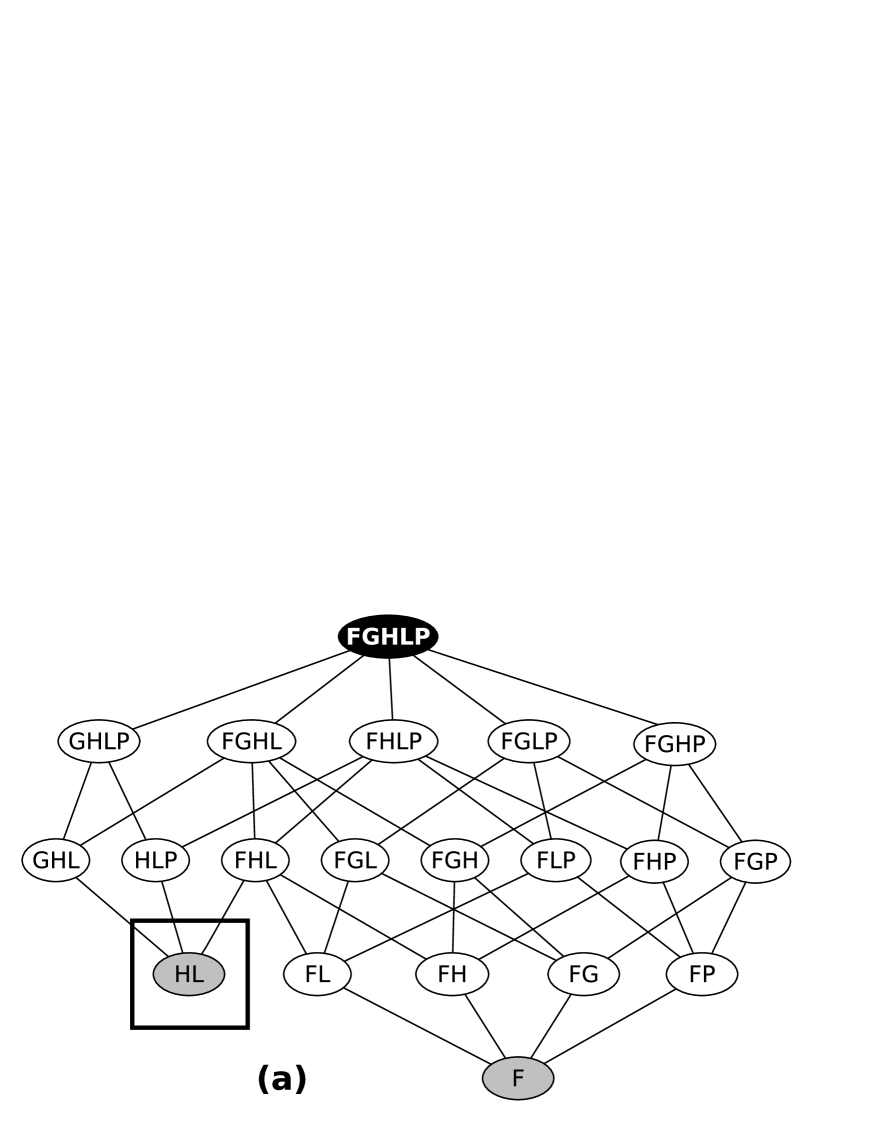
Figure 10: Evaluating Lattice in Figure 9(b)

Example 5 (Lattice Evaluation).

Consider the lattice in Fig.10(a) where the lightly shaded nodes belong to the $\mathcal{LF}$ and the darkly shaded node belongs to $\mathcal{UF}$. At the beginning, only the minimal query trees belong to the $\mathcal{LF}$ and the maximal query graph belongs to the $\mathcal{UF}$. If HL is chosen as $Q_{best}$ and evaluating it results in matching answer graphs, all its parents (GHL, HLP and FHL) are added to $\mathcal{LF}$ as shown in Fig.10(b). The evaluated node HL is represented in bold dashed node.

(2) Pruning and Lattice Recomputation

A lattice node that does not have any answer graph is referred to as a null node. If the most promising node $Q_{best}$ turns out to be a null node after evaluation, all its ancestors are also null nodes based on Property 3 below which follows directly from Property 1.

Property 3 (Upward Closure).

If $\mathcal{A}_{Q_{1}}=\emptyset$, then $\forall Q_{2}\succ Q_{1}$, $\mathcal{A}_{Q_{2}}=\emptyset$.

Proof.

Suppose there is a query node $Q_{2}$ such that $Q_{1}\prec Q_{2}$ and $\mathcal{A}_{Q_{1}}=\emptyset$, while $\mathcal{A}_{Q_{2}}\neq\emptyset$. By Property 1, for every answer graph $A$ in $\mathcal{A}_{Q_{2}}$, there must exist a subgraph of $A$ that belongs to $\mathcal{A}_{Q_{1}}$. This is a contradiction and completes the proof.

Input: query lattice $\mathcal{L}$, null node $Q_{best}$, and lower-frontier $\mathcal{LF}$

1

Output: $U(Q)$ for all $Q$ in $\mathcal{LF}$

2

3foreach $Q\in\mathcal{LF}$ do

4       $\mathcal{NB}\leftarrow\phi$; // set of new upper boundary candidates of $Q$.

5       foreach $Q^{\prime}\in\mathcal{UB}(Q)\cap\mathcal{UB}(Q_{best})$ do

6             $\mathcal{UB}(Q)\leftarrow\mathcal{UB}(Q)\setminus\{Q^{\prime}\}$;

7             $\mathcal{UF}\leftarrow\mathcal{UF}\setminus\{Q^{\prime}\}$;

8             $V(Q^{\prime\prime})\leftarrow V(Q^{\prime})$;

9             foreach $e\in E(Q_{best})\setminus E(Q)$ do

10                   $E(Q^{\prime\prime})\leftarrow E(Q^{\prime})\setminus\{e\}$;

11                   find $Q_{sub}$, the weakly-connected component of $Q^{\prime\prime}$, containing all query entities;

12                   $\mathcal{NB}\leftarrow\mathcal{NB}\cup\{Q_{sub}\}$;

13                  

14            

15      foreach $Q_{sub}\in\mathcal{NB}$ do

16             if $Q_{sub}\nprec$ (any node in $\mathcal{UF}$ or $\mathcal{NB}$) then

17                   $\mathcal{UB}(Q)\leftarrow\mathcal{UB}(Q)\cup\{Q_{sub}\}$, $\mathcal{UF}\leftarrow\mathcal{UF}\cup\{Q_{sub}\}$;

18            

19      recompute $U(Q)$ using Eq. (9);

Algorithm 3 Recomputing Upper-bound Scores

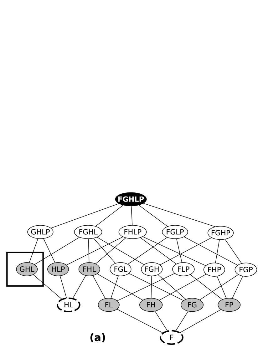
Figure 11: Recomputing Upper Boundary of Dirty Node $FG$

Based on Property 3, when $Q_{best}$ is evaluated to be a null node, Alg.2 prunes $Q_{best}$ and its ancestors, which changes the upper-frontier $\mathcal{UF}$. It is worth noting that $Q_{best}$ itself may be an upper-frontier node, in which case only $Q_{best}$ is pruned. In general, due to the evaluation and pruning of nodes, $\mathcal{LF}$ and $\mathcal{UF}$ might overlap. For nodes in $\mathcal{LF}$ that have at least one upper boundary node among the pruned ones, the change of $\mathcal{UF}$ leads to changes in their upper boundaries and, sometimes, their upper-bound scores too. We refer to such nodes as dirty nodes. The rest of this section presents an efficient method (Alg. 3) to recompute the upper boundaries, and if changed, the upper-bound scores of the dirty nodes.

Consider all the pairs $\langle Q,Q^{\prime}\rangle$ such that $Q$ is a dirty node in $\mathcal{LF}$, and $Q^{\prime}$ is one of its pruned upper boundary nodes. Three necessary conditions for a new candidate upper boundary node of $Q$ are that it is (1) a supergraph of $Q$, (2) a subgraph of $Q^{\prime}$ and (3) not a supergraph of $Q_{best}$. The subsumption relationships among these graphs can be visualized in a Venn diagram, as shown in Fig.12. If there are $q$ edges in $Q_{best}$ but not in $Q$ (the non-intersecting region of $Q_{best}$ in Fig.12), we create a set of $q$ distinct graphs $Q^{\prime\prime}$. Each $Q^{\prime\prime}$ contains all edges in $Q^{\prime}$ except exactly one of the aforementioned $q$ edges (Line 8 in Alg. 3). For each $Q^{\prime\prime}$, we find $Q_{sub}$ which is the weakly connected component of $Q^{\prime\prime}$ containing all the query entities (Lines 9-10).

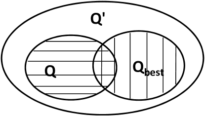
Figure 12: Venn Diagram of Edges

Lemma 1 and 2 show that $Q_{sub}$ must be one of the unevaluated nodes after pruning the ancestor nodes of $Q_{best}$ from $\mathcal{L}$.

Lemma 1.

$Q_{sub}$ is a query graph and it does not belong to the pruned nodes of lattice $\mathcal{L}$.

Proof.

$Q_{sub}$ is a query graph because it is weakly connected and it contains all the input entities. Suppose $Q_{sub}$ is a newly generated candidate upper boundary node from pair $\langle Q,Q^{\prime}\rangle$ and $Q_{sub}$ belongs to the pruned nodes of lattice $\mathcal{L}$. This can happen only due to one of the two reasons: 1) it is a supergraph of the current null node $Q_{best}$ or 2) it is an already pruned node. The former cannot happen since the construction mechanism of $Q_{sub}$ proposed ensures that it is not a supergraph of $Q_{best}$. the latter implies that $Q_{sub}$ was the supergraph of an previously evaluated null node (or $Q_{sub}$ itself was a null node). In this case, since $Q_{sub}\prec Q^{\prime}$, $Q^{\prime}$ would also have been pruned and thus could not have been part of the upper-boundary. Hence $\langle Q,Q^{\prime}\rangle$ cannot be a valid pair for recomputing the upper boundary if $Q_{sub}$ is a pruned node. This completes the proof.

Lemma 2.

$Q\preceq Q_{sub}$.

Proof.

Based on Alg. 3 described above, $Q^{\prime\prime}$ is the result of deleting one edge from $Q^{\prime}$ and that edge does not belong to $Q$. Therefore, $Q$ is subsumed by $Q^{\prime\prime}$. By the same algorithm, $Q_{sub}$ is the weakly connected component of $Q^{\prime\prime}$ that contains all the query entities. Since $Q$ already is weakly connected and contains all the query entities, $Q_{sub}$ must be a supergraph of $Q$.

If $Q_{sub}$ (a candidate new upper boundary node of $Q$) is not subsumed by any node in the upper-froniter or other candidate nodes, we add $Q_{sub}$ to $\mathcal{UB}$($Q$) and $\mathcal{UF}$ (Lines 11-13). Finally, we recompute $Q$’s upper-bound score (Line 14). Theorem 3 justifies the correctness of the above procedure.

Theorem 3.

If $Q_{best}$ is evaluated to be a null node, then Alg.3 identifies all new upper boundary nodes for every dirty node $Q$.

Proof.

For any dirty node $Q$, its original upper boundary $\mathcal{UB}(Q)$ consists of two sets of nodes: (1) nodes that are not supergraphs of $Q_{best}$ and thus remain in the lattice, (2) nodes that are supergraphs of $Q_{best}$ and thus are pruned. By the definition of upper boundary node, no upper boundary node of $Q$ can be a subgraph of any node in set (1). So any new upper boundary node of $Q$ must be a subgraph of a node $Q^{\prime}$ in set (2). For every pruned upper boundary node $Q^{\prime}$ in set (2), the algorithm enumerates all (specifically $q$) possible children of $Q^{\prime}$ that are not supergraphs of $Q_{best}$ but are supergraphs of $Q$. For each enumerated graph $Q^{\prime\prime}$, the algorithm finds $Q_{sub}$, which is the weakly connected component of $Q^{\prime\prime}$ containing all query entities. Thus all new upper boundary nodes of $Q$ are identified.

Example 6 (Recomputing Upper Boundary).

Consider the lattice in Fig.11(a) where nodes HL and F are the evaluated nodes and the lightly shaded nodes belong to the new $\mathcal{LF}$. If node GHL is the currently evaluated null node $Q_{best}$ and FGHLP is $Q^{\prime}$, let FG be the dirty node $Q$ whose upper boundary is to be recomputed. The edges in $Q_{best}$ that are not present in $Q$ are H and L. A new upper boundary node $Q^{\prime\prime}$ contains all edges in $Q^{\prime}$ excepting exactly either H or L. This leads to two new upper boundary nodes, FGHP and FGLP, by removing L and H from FGHLP, respectively. Since FGHP and FGLP do not subsume each other and are not subgraphs of any other upper-frontier node, they are now part of $\mathcal{UB}$($Q$) and the new $\mathcal{UF}$. Fig.11(b) shows the modified lattice where the pruned nodes are disconnected. FHLP is another node in $\mathcal{UF}$ that is discovered using dirty nodes such as FL and HLP.

Complexity Analysis of Alg.3   The query graphs corresponding to lattice nodes are represented using bit vectors since we exactly know the edges involved in all the query graphs. The bit corresponding to an edge is set if its present in the query graph. Identifying the dirty nodes, null upper boundary nodes and building a new potential upper boundary node using a pair of nodes $\langle Q,Q^{\prime}\rangle$, can be accomplished using bit operations and each step incurs $O(\lvert{E(MQG_{t})}\lvert)$ time. Finding the weakly connected component of a potential upper boundary using DFS takes $O(\lvert{E(Q^{\prime})}\lvert)$ time. If $\mathcal{L}_{n}$ is the set of all null nodes encountered in the lattice and there are $D_{p}$ such pairs for every null node and $q$ is the average number of potential new upper boundary nodes created per pair, the worst case time complexity of recomputing the upper-frontier is $O(\lvert\mathcal{L}_{n}\lvert\times D_{p}\times q\times\lvert{E(MQG_{t})}\lvert)$. Our experimental results show low average values of $\lvert\mathcal{L}_{n}\lvert$, $D_{p}$ and $q$ with $\lvert\mathcal{L}_{n}\lvert$ being only 1% of $\lvert\mathcal{L}\lvert$, $D_{p}$ around 8 and $q$ around 9. In practice, our upper-frontier recomputation algorithm quickly computes the dynamically changing lattice.

(3) Termination

After $Q_{best}$ is evaluated, its answer tuples are $\{t_{A}|A$$\in$$\mathcal{A}_{Q_{best}}\}$. For a $t_{A}$ projected from answer graph $A$, the score assigned by $Q_{best}$ to $A$ (and thus $t_{A}$) is $\textsf{s\_score}(Q_{best})$, based on ${\textsf{score}_{Q}}(A)$$=$${\textsf{s\_score}}(Q)$—the simplified scoring function adopted by Alg.2. If $t_{A}$ was also projected from already evaluated nodes, it has a current score. By Def.4, the final score of $t_{A}$ will be from its best answer graph. Hence, if $\textsf{s\_score}(Q_{best})$ is higher than its current score, then its score is updated. In this way, all found answer tuples so far are kept and their current scores are maintained to be the highest scores they have received. The algorithm terminates when the current score of the $k^{th}$ best answer tuple so far is greater than the upper-bound score of the next $Q_{best}$ chosen by the algorithm, by Theorem 4.

Theorem 4.

If the score of the current $k^{th}$ best answer tuple is greater than $U(Q_{best})$, then terminating the lattice evaluation guarantees that the current top-$k$ answer tuples have scores higher than $\textsf{s\_score}(Q)$ for any unevaluated query graph $Q$.

Proof.

Suppose, upon termination, there is an unevaluated query graph $Q$ whose $\textsf{s\_score}(Q)$ is greater than the score of the $k^{th}$ answer tuple. This implies that there exists some node in the lower-frontier whose upper-bound score is at least $\textsf{s\_score}(Q)$ and is thus greater than the score of the $k^{th}$ answer tuple. Since the termination condition precludes this, it is a contradiction to the initial assumption. We thus cannot have any unevaluated query graph whose structure score is greater than the $k^{th}$ answer tuple’s score upon termination.

VI Experiments

This section presents our experiment results on the accuracy and efficiency of $\mathsf{GQBE}$. The experiments were conducted on a double quad-core $24$ GB Memory $2.0$ GHz Xeon server.

Query	Query Tuple	Table Size
F1	$\langle$Donald Knuth, Stanford University, Turing Award$\rangle$	18
F2	$\langle$Ford Motor, Lincoln, Lincoln MKS$\rangle$	25
F3	$\langle$Nike, Tiger Woods$\rangle$	20
F4	$\langle$Michael Phelps, Sportsman of the Year$\rangle$	55
F5	$\langle$Gautam Buddha, Buddhism$\rangle$	621
F6	$\langle$Manchester United, Malcolm Glazer$\rangle$	40
F7	$\langle$Boeing, Boeing C-22$\rangle$	89
F8	$\langle$David Beckham, A. C. Milan$\rangle$	94
F9	$\langle$Beijing, 2008 Summer Olympics$\rangle$	41
F10	$\langle$Microsoft, Microsoft Office$\rangle$	200
F11	$\langle$Jack Kirby, Ironman$\rangle$	25
F12	$\langle$Apple Inc, Sequoia Capital$\rangle$	300
F13	$\langle$Beethoven, Symphony No. 5$\rangle$	600
F14	$\langle$Uranium, Uranium-238$\rangle$	26
F15	$\langle$Microsoft Office, C++$\rangle$	300
F16	$\langle$Dennis Ritchie, C$\rangle$	163
F17	$\langle$Steven Spielberg, Minority Report$\rangle$	40
F18	$\langle$Jerry Yang, Yahoo!$\rangle$	8349
F19	$\langle$C$\rangle$	1240
F20	$\langle$TomKat$\rangle$	16
D1	$\langle$Alan Turing, Computer Scientist$\rangle$	52
D2	$\langle$David Beckham, Manchester United$\rangle$	273
D3	$\langle$Microsoft, Microsoft Excel$\rangle$	300
D4	$\langle$Steven Spielberg, Catch Me If You Can$\rangle$	37
D5	$\langle$Boeing C-40 Clipper, Boeing$\rangle$	118
D6	$\langle$Arnold Palmer, Sportsman of the year$\rangle$	251
D7	$\langle$Manchester City FC, Mansour bin Zayed Al Nahyan$\rangle$	40
D8	$\langle$Bjarne Stroustrup, C++$\rangle$	964

TABLE I: Queries and Ground Truth Table Size

Datasets

The experiments were conducted over two large real-world knowledge graphs, the Freebase [4] and DBpedia [3] datasets. We preprocessed the graphs so that the kept nodes are all named entities (e.g., Stanford University) and abstract concepts (e.g., Jewish people). The resulting Freebase graph contains $28$M nodes, $47$M edges, and $5,428$ distinct edge labels. The DBpedia graph contains $759$K nodes, $2.6$M edges and $9,110$ distinct edge labels.

Methods Compared

$\mathsf{GQBE}$ was compared with a $\mathsf{Baseline}$ and $\mathsf{NESS}$ [18]. $\mathsf{NESS}$ is a graph querying framework that finds approximate matches of query graphs with unlabeled nodes which correspond to query entity nodes in MQG. Note that, like other systems, $\mathsf{NESS}$ must take a query graph (instead of a query tuple) as input. Hence, we feed the MQG discovered by $\mathsf{GQBE}$ as the query graph to $\mathsf{NESS}$. For each node $v$ in the query graph, a set of candidate nodes in the data graph are identified. Since, $\mathsf{NESS}$ does not consider edge-labeled graphs, we adapted it by requiring each candidate node $v^{\prime}$ of $v$ to have at least one incident edge in the data graph bearing the same label of an edge incident on $v$ in the query graph. The score of a candidate $v^{\prime}$ is the similarity between the neighborhoods of $v$ and $v^{\prime}$, represented in the form of vectors, and further refined using an iterative process. Finally, one unlabeled query node is chosen as the pivot $p$. The top-$k$ candidates for multiple unlabeled query nodes are put together to form answer tuples, if they are within the neighborhood of $p$’s top-$k$ candidates. Similar to the best-first method (Sec.V), $\mathsf{Baseline}$ explores a query lattice in a bottom-up manner and prunes ancestors of null nodes. However, differently, it evaluates the lattice by breadth-first traversal instead of in the order of upper-bound scores. There is no early-termination by top-k scores, as $\mathsf{Baseline}$ terminates when every node is either evaluated or pruned. We implemented $\mathsf{GQBE}$ and $\mathsf{Baseline}$ in Java and we obtained the source code of $\mathsf{NESS}$ from the authors.

Queries and Ground Truth

Two groups of queries are used on the two datasets, respectively. The Freebase queries F₁– F₂₀ are based on Freebase tables such as http:// www.freebase.com/view/computer/programming_language_designer?instances, except F₁ and F₆ which are from Wikipedia tables such as http://en.wikipedia.org/wiki/List_of_English_football_club_owners. The DBpedia queries D₁– D₈ are based on DBpedia tables such as the values for property is dbpedia-owl:author of on page http://dbpedia.org/page/Microsoft. Each such table is a collection of tuples, in which each tuple consists of one, two, or three entities. For each table, we used one or more tuples as query tuples and the remaining tuples as the ground truth for query answers. All the $28$ queries and their corresponding table sizes are summarized in Table I. They cover diverse domains, including people, companies, movies, sports, awards, religions, universities and automobiles.

Query Tuple	Top-$3$ Answer Tuples
	$\langle$D. Knuth, Stanford, V. Neumann Medal$\rangle$
$\langle$Donald Knuth, Stanford, Turing Award$\rangle$	$\langle$J. McCarthy, Stanford, Turing Award$\rangle$
	$\langle$N. Wirth, Stanford, Turing Award$\rangle$
	$\langle$David Filo, Yahoo!$\rangle$
$\langle$Jerry Yang, Yahoo!$\rangle$	$\langle$Bill Gates, Microsoft$\rangle$
	$\langle$Steve Wozniak, Apple Inc.$\rangle$
	$\langle$Java$\rangle$
$\langle$C$\rangle$	$\langle$C++$\rangle$
	$\langle$C Sharp$\rangle$

TABLE II: Case Study: Top-$3$ Results for Selected Queries

Sample Answers

Table II only lists the top-$3$ results found by $\mathsf{GQBE}$ for $3$ queries (F₁, F₁₈, F₁₉), due to space limitations.

(A) Accuracy Based on Ground Truth

We measured the accuracy of $\mathsf{GQBE}$ and $\mathsf{NESS}$ by comparing their query results with the ground truth. The accuracy on a set of queries is the average of accuracy on individual queries. The accuracy on a single query is captured by three widely-used measures [23], as follows.

• Precision-at-$k$ (P@$k$): the percentage of the top-$k$ results that belong to the ground truth.

• Mean Average Precision (MAP): The average precision of the top-$k$ results is AvgP$=$$\frac{\sum_{i=1}^{k}{\text{P}@i}\ \times\ rel_{i}}{\text{size of ground truth}}$, where $rel_{i}$ equals $1$ if the result at rank $i$ is in the ground truth and $0$ otherwise. MAP is the mean of AvgP for a set of queries.

• Normalized Discounted Cumulative Gain (nDCG): The cumulative gain of the top-$k$ results is DCG_k$=$$rel_{1}$$+$$\sum_{i=2}^{k}{\frac{rel_{i}}{\log_{2}(i)}}$. It penalizes the results if a ground truth result is ranked low. DCG_k is normalized by IDCG_k, the cumulative gain for an ideal ranking of the top-$k$ results. Thus nDCG_k$=$$\frac{\text{DCG}_{k}}{\text{IDCG}_{k}}$.

(a) P@$k$

(b) MAP

(c) nDCG

Figure 13: Accuracy of $\mathsf{GQBE}$ and $\mathsf{NESS}$ on Freebase Queries

Query	P@$k$	nDCG	AvgP	Query	P@$k$	nDCG	AvgP
D1	1.00	1.00	0.20	D2	1.00	1.00	0.04
D3	1.00	1.00	0.03	D4	0.80	0.94	0.19
D5	0.90	1.00	0.08	D6	1.00	1.00	0.04
D7	0.90	0.98	0.22	D8	1.00	1.00	0.01

TABLE III: Accuracy of $\mathsf{GQBE}$ on DBpedia Queries, $k$=$10$

Fig.13 shows these measures for different values of $k$ on the Freebase queries. $\mathsf{GQBE}$ has high accuracy. For instance, its P@$25$ is over $0.8$. The absolute value of MAP is not high, merely because Fig.13(b) only shows the MAP for at most top-$25$ results, while the ground truth size (i.e., the denominator in calculating MAP) for many queries is much larger. Moreover, $\mathsf{GQBE}$ outperforms $\mathsf{NESS}$ substantially, as its accuracy in all three measures is almost always twice as better. This is because $\mathsf{GQBE}$ gives priority to query entities and important edges in MQG, while $\mathsf{NESS}$ gives equal importance to all nodes and edges except the pivot. Furthermore, the way $\mathsf{NESS}$ handles edge labels does not explicitly require answer entities to be connected by the same paths between query entities.

Table III further shows the accuracy of $\mathsf{GQBE}$ on individual DBpedia queries at $k$=$10$. It exhibits high accuracy on all queries, including perfect precision in several cases.

Query	PCC	Query	PCC	Query	PCC	Query	PCC
F1	0.79	F2	0.78	F3	0.60	F4	0.80
F5	0.34	F6	0.27	F7	0.06	F8	0.26
F9	0.33	F10	0.77	F11	0.58	F12	undefined
F13	undefined	F14	0.62	F15	0.43	F16	0.29
F17	0.64	F18	0.30	F19	0.40	F20	0.65

TABLE IV: Pearson Correlation Coefficient (PCC) between $\mathsf{GQBE}$ and Amazon MTurk Workers, $k$=$30$

(B) Accuracy Based on User Study

We conducted an extensive user study through Amazon Mechanical Turk (MTurk, https://www.mturk.com/mturk/) to evaluate $\mathsf{GQBE}$’s accuracy on Freebase queries, measured by Pearson Correlation Coefficient (PCC). For each of the $20$ queries, we obtained the top-$30$ answers from $\mathsf{GQBE}$ and generated $50$ random pairs of these answers. We presented each pair to $20$ MTurk workers and asked for their preference between the two answers in the pair. Hence, in total, $20,000$ opinions were obtained. We then constructed two value lists per query, $X$ and $Y$, which represent $\mathsf{GQBE}$ and MTurk workers’ opinions, respectively. Each list has $50$ values, for the $50$ pairs. For each pair, the value in $X$ is the difference between the two answers’ ranks given by $\mathsf{GQBE}$, and the value in $Y$ is the difference between the numbers of workers favoring the two answers. The PCC value for a query is $(\text{E}(XY)-\text{E}(X)\text{E}(Y))/(\sqrt{\text{E}(X^{2})-(\text{E}(X))^{2}}\sqrt{\text{E}(Y^{2})-(\text{E}(Y))^{2}})$. The value indicates the degree of correlation between the pairwise ranking orders produced by $\mathsf{GQBE}$ and the pairwise preferences given by MTurk workers. The value range is from $-1$ to $1$. A PCC value in the ranges of [$0.5$,$1.0$], [$0.3$,$0.5$) and [$0.1$,$0.3$) indicates a strong, medium and small positive correlation, respectively [7]. PCC is undefined, by definition, when $X$ and/or $Y$ contain all equal values.

Table IV shows the PCC values for F₁-F₂₀. Out of the $20$ queries, $\mathsf{GQBE}$ attained strong, medium and small positive correlation with MTurk workers on $9$, $5$ and $3$ queries, respectively. Only query F₇ shows no correlation. Note that PCC is undefined for F₁₂ and F₁₃, because all the top-$30$ answer tuples have the same score and thus the same rank, resulting in all zero values in $X$, i.e., $\mathsf{GQBE}$’s list.

Query	Tuple1			Tuple2			Combined (1,2)			Tuple3			Combined (1,2,3)
	P@$k$	nDCG	AvgP	P@$k$	nDCG	AvgP	P@$k$	nDCG	AvgP	P@$k$	nDCG	AvgP	P@$k$	nDCG	AvgP
F1	0.36	0.76	0.32	0.36	1.00	0.50	0.12	0.38	0.02	0.36	0.73	0.22	0.12	0.49	0.02
F2	0.76	1.00	0.79	0.00	0.00	0.00	0.80	1.00	0.80	0.12	0.70	0.05	0.80	1.00	0.91
F4	0.32	0.73	0.09	0.40	0.65	0.08	1.00	1.00	0.45	N/A	N/A	N/A	N/A	N/A	N/A
F6	0.24	0.89	0.16	0.28	0.89	0.18	0.40	0.87	0.16	0.36	0.98	0.22	0.12	0.94	0.07
F8	0.92	0.79	0.20	1.00	1.00	0.27	0.96	0.98	0.24	0.48	0.86	0.08	1.00	1.00	0.27
F9	0.68	0.72	0.23	0.56	0.66	0.17	0.80	0.86	0.35	1.00	1.00	0.62	1.00	1.00	0.66
F17	0.32	1.00	0.33	0.64	0.83	0.25	0.32	1.00	0.32	0.56	0.84	0.23	0.68	1.00	0.46

TABLE V: Accuracy of $\mathsf{GQBE}$ on Multi-tuple Queries, $k$=$25$

Figure 14: Query Processing Time

Figure 15: Lattice Nodes Evaluated

(C) Accuracy on Multi-tuple Queries

We investigated the effectiveness of the multi-tuple querying approach (Sec.III-D). In aforementioned single-tuple query experiment (A), $\mathsf{GQBE}$ attained perfect P@$25$ for $13$ of the $20$ Freebase queries. We thus focused on the remaining $7$ queries. For each query, Tuple1 refers to the query tuple in Table I, while Tuple2 and Tuple3 are two tuples from its ground truth. Table V shows the accuracy of top-$25$ $\mathsf{GQBE}$ answers for the three tuples individually, as well as for the first two and three tuples together by merged MQGs, which are denoted Combined(1,2) and Combined(1,2,3), respectively. F₄ attained perfect precision after Tuple2 was included. Therefore, Tuple3 was not used for F₄. The results show that, in most cases, Combined(1,2) had better accuracy than individual tuples and Combined(1,2,3) further improved accuracy.

(D) Efficiency Results

We compared the efficiency of $\mathsf{GQBE}$, $\mathsf{NESS}$ and $\mathsf{Baseline}$ on Freebase queries. The total run time for a query tuple is spent on two components—query graph discovery and query processing. Fig.15 compares the three methods’ query processing time, in logarithmic scale. The figure shows the query processing time for each of the $20$ Freebase queries, and the edge cardinality of the MQG for each of those is shown below the corresponding query id. The query cost does not appear to increase by edge cardinality, regardless of the query method. For $\mathsf{GQBE}$ and $\mathsf{Baseline}$, this is because query graphs are evaluated by joins and join selectivity plays a more significant role in evaluation cost than number of edges. $\mathsf{NESS}$ finds answers by intersecting postings lists on feature vectors. Hence, in evaluation cost, intersection size matters more than edge cardinality. $\mathsf{GQBE}$ outperformed $\mathsf{NESS}$ on $17$ of the $20$ queries and was more than $3$ times faster in $10$ of them. It finished within $10$ seconds on $17$ queries. However, it performed very poorly on F$4$ and F$19$, which have $10$ and $7$ edges respectively. This indicates that the edges in the two MQGs lead to poor join selectivity. $\mathsf{Baseline}$ clearly suffered, due to its inferior pruning power compared to the best-first exploration employed by $\mathsf{GQBE}$. This is evident in Fig.15 which shows the numbers of lattice nodes evaluated for each query. $\mathsf{GQBE}$ evaluated considerably less nodes in most cases and at least $2$ times less on $11$ of the $20$ queries.

MQG discovery precedes the query processing step and is shared by all three methods. Column MQG₁ in Table VI lists the time spent on discovering MQG for each Freebase query. This time component varies across individual queries, depending on the sizes of query tuples’ neighborhood graphs. Compared to the values shown in Fig.15, the time taken to discover an MQG in average is comparable to the time spent by $\mathsf{GQBE}$ in evaluating it.

Query	MQG1	MQG2	Merge	Query	MQG1	MQG2	Merge
F1	73.141	73.676	0.034	F2	0.049	0.029	0.006
F3	12.566	4.414	0.024	F4	5.731	7.083	0.024
F5	9.982	2.522	0.079	F6	6.082	4.654	0.039
F7	0.152	0.107	0.007	F8	10.272	2.689	0.032
F9	62.285	2.384	0.041	F10	2.910	5.933	0.030
F11	59.541	65.863	0.032	F12	1.977	0.021	0.006
F13	9.481	5.624	0.034	F14	0.038	0.015	0.004
F15	0.154	5.143	0.021	F16	54.870	6.928	0.057
F17	60.582	69.961	0.041	F18	58.807	75.128	0.053
F19	0.224	0.076	0.003	F20	0.025	0.017	0.002

TABLE VI: Time for Discovering and Merging MQGs (secs.)

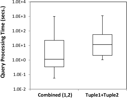
Figure 16: Query Processing Time of $2$-tuple Queries

Fig.16 shows the distribution of the $\mathsf{GQBE}$’s query processing time, in logarithmic scale, on the merged MQGs of 2-tuple queries in Table V, denoted by Combined(1,2). It also shows the distribution of the total time for evaluating the two tuples’ MQGs individually, denoted Tuple1+Tuple2. Combined(1,2) processes $10$ of the $20$ queries in less than a second while the fastest query for Tuple1+Tuple2 takes a second. This suggests that the merged MQGs gave higher weights to more selective edges, resulting in faster lattice evaluation. Meanwhile, these selective edges are also more important edges common to the two query tuples, leading to improved answer accuracy as shown in Table V. Table VI further shows the time taken to discover MQG₁ and MQG₂ for the two tuples, along with the time for merging them. The latter is negligible compared to the former.

VII Related Work

Lim et al. [21] use example tuples to find similar tuples in database tables that are coupled with ontologies. They do not deal with graph data and the example tuples are not formed by entities.

The goal of set expansion is to grow a set of objects starting from seed objects. Example systems include [30], [11], and the now defunct $\mathsf{Google\ Sets}$ and $\mathsf{Squared}$ services (http://en.wikipedia.org/wiki/List_of_Google_products). Chang et al. [5] identify top-k correlated keyword terms from an information network given a set of terms, where each term can be an entity. These systems, except [5], do not operate on data graphs. Instead, they find existing answers within structures in web pages such as HTML tables and lists. Furthermore, all these systems except $\mathsf{Google\ Squared}$ and [11] take a set of individual entities as input. $\mathsf{GQBE}$ is more general in that each query tuple contains multiple entities.

Several works [28, 17, 9] identify the best subgraphs/paths in a data graph to describe how several input nodes are related. The query graph discovery component of $\mathsf{GQBE}$ is different in important ways– (1) The graphs in [28] contain nodes of the same type and edges representing the same relationship, e.g., social networks capturing friendship between people. The graphs in $\mathsf{GQBE}$ and others [17, 9] have many different types of entities and relationships. (2) The paths discovered by their techniques only connect the input nodes. $\mathsf{REX}$ [9] has the further limitation of allowing only two input entities. Differently the maximal query graph in $\mathsf{GQBE}$ includes edges incident on individual query entities. (3) $\mathsf{GQBE}$ uses the discovered query graph to find answer graphs and answer tuples, which is not within the focus of the aforementioned works.

There are many studies on approximate/inexact subgraph matching in large graphs, such as $\mathsf{G}$-$\mathsf{Ray}$ [29], $\mathsf{TALE}$ [27] and $\mathsf{NESS}$ [18]. $\mathsf{GQBE}$’s query processing component is different from them on several aspects. First, $\mathsf{GQBE}$ only requires to match edge labels and matching node identifiers is not mandatory. This is equivalent to matching a query graph with all unlabeled nodes and thereby significantly increases the problem complexity. Only a few previous methods (e.g., $\mathsf{NESS}$ [18]) allow unlabeled query nodes. Second, in $\mathsf{GQBE}$, the top-k query algorithm centers around query entities. More specifically, the weighting function gives more importance to query entities and the minimal query trees mandate the presence of entities corresponding to query entities. On the contrary, previous methods give equal importance to all nodes in a query graph, since the notion of query entity does not exist there. Our empirical results show that this difference makes $\mathsf{NESS}$ produce less accurate answers than $\mathsf{GQBE}$. Finally, although the query relaxation DAG proposed in [2] is similar to $\mathsf{GQBE}$’s query lattice, the scoring mechanism of their relaxed queries is different and depends on XML-based relaxations.

VIII Conclusion

We introduce $\mathsf{GQBE}$, a system that queries knowledge graphs by example entity tuples. As an initial step toward better usability of graph query systems, $\mathsf{GQBE}$ saves users the burden of forming explicit query graphs. To the best of our knowledge, there has been no such proposal in the past. Its query graph discovery component derives a hidden query graph based on example tuples. The query lattice based on this hidden graph may contain a large number of query graphs. $\mathsf{GQBE}$’s query algorithm only partially evaluates query graphs for obtaining the top-k answers. Experiments on Freebase and DBpedia datasets show that $\mathsf{GQBE}$ outperforms the state-of-the-art system $\mathsf{NESS}$ on both accuracy and efficiency.

IX Acknowledgements

The authors would like to thank Mahesh Gupta for his valuable contributions in performing the experiments.

References

- [1] D. J. Abadi, A. Marcus, S. Madden, and K. J. Hollenbach. Scalable semantic web data management using vertical partitioning. In VLDB’07.
- [2] S. Amer-Yahia, N. Koudas, A. Marian, D. Srivastava, and D. Toman. Structure and content scoring for xml. In VLDB, 2005.
- [3] S. Auer, C. Bizer, G. Kobilarov, J. Lehmann, R. Cyganiak, and Z. Ives. DBpedia: A nucleus for a Web of open data. In ISWC, 2007.
- [4] K. Bollacker, C. Evans, P. Paritosh, T. Sturge, and J. Taylor. Freebase: a collaboratively created graph database for structuring human knowledge. In SIGMOD, pages 1247–1250, 2008.
- [5] L. Chang, J. X. Yu, L. Qin, Y. Zhu, and H. Wang. Finding information nebula over large networks. In CIKM, 2011.
- [6] D. H. Chau, C. Faloutsos, H. Tong, J. I. Hong, B. Gallagher, and T. Eliassi-Rad. GRAPHITE: A visual query system for large graphs. In ICDM Workshops, pages 963–966, 2008.
- [7] J. Cohen. Statistical Power Analysis for the Behavioral Sciences. Lawrence Erlbaum Associates, 1988.
- [8] E. Demidova, X. Zhou, and W. Nejdl. FreeQ: an interactive query interface for Freebase. In WWW, demo paper, 2012.
- [9] L. Fang, A. D. Sarma, C. Yu, and P. Bohannon. REX: explaining relationships between entity pairs. In PVLDB, pages 241–252, 2011.
- [10] H. N. Gabow and E. W. Myers. Finding all spanning trees of directed and undirected graphs. SIAM J. Comput., 7(3):280–287, 1978.
- [11] R. Gupta and S. Sarawagi. Answering table augmentation queries from unstructured lists on the web. In VLDB, pages 289–300, 2009.
- [12] H. V. Jagadish, A. Chapman, A. Elkiss, M. Jayapandian, Y. Li, A. Nandi, and C. Yu. Making database systems usable. In SIGMOD, 2007.
- [13] M. Jarrar and M. D. Dikaiakos. A query formulation language for the data web. TKDE, 24:783–798, 2012.
- [14] N. Jayaram, M. Gupta, A. Khan, C. Li, X. Yan, and R. Elmasri. GQBE: Querying knowledge graphs by example entity tuples. In ICDE (demo description), 2014 (to appear).
- [15] C. Jin, S. S. Bhowmick, X. Xiao, J. Cheng, and B. Choi. GBLENDER: Towards blending visual query formulation and query processing in graph databases. In SIGMOD, pages 111–122, 2010.
- [16] M. Kargar and A. An. Keyword search in graphs: Finding r-cliques. PVLDB, pages 681–692, 2011.
- [17] G. Kasneci, S. Elbassuoni, and G. Weikum. MING: mining informative entity relationship subgraphs. In CIKM, 2009.
- [18] A. Khan, N. Li, X. Yan, Z. Guan, S. Chakraborty, and S. Tao. Neighborhood based fast graph search in large networks. In SIGMOD’11.
- [19] A. Khan, Y. Wu, and X. Yan. Emerging graph queries in linked data. In ICDE, pages 1218–1221, 2012.
- [20] Z. Li, S. Zhang, X. Zhang, and L. Chen. Exploring the constrained maximum edge-weight connected graph problem. Acta Mathematicae Applicatae Sinica, 25:697–708, 2009.
- [21] L. Lim, H. Wang, and M. Wang. Semantic queries by example. In Proceedings of the 16th International Conference on Extending Database Technology (EDBT 2013), 2013.
- [22] Y. Luo, X. Lin, W. Wang, and X. Zhou. Spark: top-k keyword query in relational databases. In SIGMOD, 2007.
- [23] C. D. Manning, P. Raghavan, and H. Schtze. Introduction to Information Retrieval. Cambridge University Press, NY, USA, 2008.
- [24] J. Pound, I. F. Ilyas, and G. E. Weddell. Expressive and flexible access to web-extracted data: a keyword-based structured query language. In SIGMOD, pages 423–434, 2010.
- [25] F. M. Suchanek, G. Kasneci, and G. Weikum. YAGO: a core of semantic knowledge unifying WordNet and Wikipedia. In WWW, 2007.
- [26] Y. Sun, J. Han, X. Yan, P. S. Yu, , and T. Wu. PathSim: Meta path-based top-k similarity search in heterogeneous information networks. VLDB, 2011.
- [27] Y. Tian and J. M. Patel. TALE: A tool for approximate large graph matching. In ICDE, pages 963–972, 2008.
- [28] H. Tong and C. Faloutsos. Center-piece subgraphs: Problem definition and fast solutions. In KDD, pages 404–413, 2006.
- [29] H. Tong, C. Faloutsos, B. Gallagher, and T. Eliassi-Rad. Fast best-effort pattern matching in large attributed graphs. KDD, 2007.
- [30] R. C. Wang and W. W. Cohen. Language-independent set expansion of named entities using the web. In ICDM, pages 342–350, 2007.
- [31] W. Wu, H. Li, H. Wang, and K. Q. Zhu. Probase: a probabilistic taxonomy for text understanding. In SIGMOD, pages 481–492, 2012.
- [32] M. Yahya, K. Berberich, S. Elbassuoni, M. Ramanath, V. Tresp, and G. Weikum. Deep answers for naturally asked questions on the web of data. In WWW, demo paper, pages 445–449, 2012.
- [33] J. Yao, B. Cui, L. Hua, and Y. Huang. Keyword query reformulation on structured data. ICDE, pages 953–964, 2012.
- [34] X. Yu, Y. Sun, P. Zhao, and J. Han. Query-driven discovery of semantically similar substructures in heterogeneous networks. In KDD’12.
- [35] M. M. Zloof. Query by example. In AFIPS, 1975.