Dark soliton in quasi-one-dimensional Bose-Einstein condensates
with a Gaussian trap

Abstract

In this paper we study dark solitons in quasi-one-dimensional Bose-Einstein condensates (BECs) in presence of an anharmonic external potential. The theoretical model is based on the Muñoz-Mateo & Delgado (MMD) equation that describes cigar-shaped BECs with repulsive interatomic interactions. Since MMD equation presents a nonpolynomial form, the soliton-sound recombination cannot display the same pattern presented in the cubic model. We perform numerical simulations to compare both cases.

I Introduction

Solitons are localized structures that emerge from a perfect balance between the dispersive and nonlinear effects in the system Kivshar03 . In special, dark solitons are characterized by a depression in the ambient density and a phase slip. This type of soliton is divided into two classes: the black ones, for which the minimum density is zero, and the gray ones, for which the dip in the density is greater than zero. They were experimentally realized in nonlinear optics KrokelPRL88 , shallow liquids DenardoPRL90 , magnetic films ChenPRL93 , ultracold atomic Bose-Einstein condensates (BECs) BurgerPRL99 ; DenschlagSCI00 ; AndersonPRL01 , etc. In particular, BECs with repulsive interatomic interaction are prone to generation of dark solitons by various methods, e.g., by imprinting spatial phase distribution DenschlagSCI00 , by inducing density defects in BEC DuttonSCI01 , and by colision of two condensates ReinhardtJPB97 ; ScottJPB98 .

Differently from the case of attractive interatomic interaction, where bright solitons emerge without necessity of an external potential, due to the repulsive nature of atoms dark solitons requires an external confining potential. Indeed, the harmonic potentials were used in the experiments with BECs BurgerPRL99 ; DenschlagSCI00 ; AndersonPRL01 . Also, for zero temperature in 1D regime, dark solitons are stable and only solitons with zero velocity in the trap center do not move, otherwise they oscillate along the trap axis BurgerPRL99 ; BuschPRL00 . On the other hand, dark soliton propagating in an inhomogeneous condensate has also been predicted to be unstable to the emission of sound waves HuangPRA02 ; ParkerPRA10 . Recently, in Ref. ParkerPRA10 was shown that such anharmonicities could break the soliton-sound equilibrium and lead to the net decay of the soliton on a considerably shorter time scale than other dissipation mechanisms.

In this paper we study numerically the effects of soliton-sound recombination in presence of two different potentials: harmonic and Gaussian. Here, differently from Refs. ParkerPRA10 ; ParkerPRL03 ; ProukakisPRL04 , we will use the Muñoz-Mateo & Delgado (MMD) equation MMDPRA08 ; MateoPRA07 , which is an effective one-dimensional (1D) equation that governs the axial dynamics of mean-field cigar-shaped condensates with repulsive interatomic interactions, accounting accurately for the contribution from the transverse degrees of freedom. To obtain this equation, in Ref. MMDPRA08 the authors have used the standard adiabatic approximation and an accurate analytical expression for the corresponding local chemical potential in terms of the longitudinal density of the condensate, expression which determine the form of the nonlinearity MateoPRA07 (see next section).

The paper is organized as follows: in the next section we revisit the theoretical model to obtain the 1D reduction of 3D Gross-Pitaevskii equation according to Ref. MMDPRA08 ; in sec. III, we show the numerical procedure, considering the evolution of the “soliton part” and the “background part”, separately; the results are shown in sec. IV for different patterns of potential; comments and conclusion are displayed in sec. V.

II Theoretical Model

The behavior of the wave function $\Psi(\mathbf{r},t)$ of the BEC considering two-body interatomic interaction is well described by the 3D Gross-Pitaevskii (GP) equation Pethick02

$$i\hbar\frac{\partial\Psi}{\partial t}=-\frac{\hbar^{2}}{2m}\nabla^{2}\Psi+V(\mathbf{r})\Psi+gN|\Psi|^{2}\Psi,$$ (1)

where $N$ is the number of atoms in the BEC, $g=4\pi\hbar^{2}a/m$ is the interaction strength, $a$ is the s-wave scattering length, $m$ is the mass of the atomic specie, and $V(\mathbf{r})$ is the external potential. In a cigar-shaped configuration, i.e., when the frequency of transverse confinement is greater than the longitudinal one ($\omega_{\perp}\gg\omega_{x}$), the wave function can be considered with the form $\Psi(\mathbf{r},t)=\varphi(\mathbf{r_{\perp}};n(x,t))\phi(x,t),$ where $\varphi$ and $\phi$ are the transversal and longitudinal wave functions, $\mathbf{r_{\perp}}=(y,z)$, and $n(x,t)$ is the local density per unit length characterizing the axial configuration $n\equiv N\int d^{2}\mathbf{r_{\perp}}|\Psi|^{2}=N|\phi|^{2}$, since we have considered the wave function normalized to unity. In this scenario, cf. Ref. MMDPRA08 , the transversal wave function is adjusted instantaneously to the lowest-energy configuration compatible with the axial configuration at each instant of time (adiabatic approximation). Next, substituting the factorized wave function into the GPE, with the potential given by $V(\mathbf{r})=V_{\perp}(r_{\perp})+V_{x}(x)$, multiplying by $\varphi^{*}$ and integrating on the transverse coordinates $\mathbf{r_{\perp}}$, one obtains

$$i\hbar\frac{\partial\phi}{\partial t}=-\frac{\hbar^{2}}{2m}\frac{\partial^{2}\phi}{\partial x^{2}}+V_{x}\phi+\mu_{\perp}(n)\phi,$$ (2)

where we follow the definition of Ref. MMDPRA08 for the transversal chemical potential with the form

$$\mu_{\perp}\equiv\int d^{2}r_{\perp}\varphi^{*}\left[-\frac{\hbar^{2}}{2m}\nabla_{\perp}^{2}+V_{\perp}+ng|\varphi|^{2}\right]\varphi.$$ (3)

Then, one can find analytical solutions for $\mu_{\perp}$ in the Eq. (3) for the two limit cases $an\ll 1$ and $an\gg 1$, such that the dimensionless chemical potential takes the form $\overline{\mu}_{\perp}=1+2an$ (Gaussian approximation) and $\overline{\mu}_{\perp}=2\sqrt{an}$ (Thomas-Fermi approximation), respectively. According to Ref. MateoPRA07 , by using a suitable approximation scheme one can obtain $\overline{\mu}_{\perp}=\sqrt{1+4an}$, that provide the ground-state properties of any mean-field scalar Bose-Einstein condensate with short-range repulsive interatomic interactions, confined in arbitrary cigar-shaped cylindrically symmetric harmonic traps. In this case, we can conveniently rewrite the Eq. (2) in the dimensionless form

$$i\frac{\partial\psi}{\partial t}=-\frac{1}{2}\frac{\partial^{2}\psi}{\partial x^{2}}+\overline{V_{x}}\psi+\lambda\sqrt{1+\sigma|\psi|^{2}}\psi,$$ (4)

where we have considered $\phi=\psi/\sqrt{l_{x}}$, $t\rightarrow t/\omega_{x}$, $x\rightarrow xl_{x}$, $V_{x}=\hbar\omega_{x}\overline{V_{x}}$, $a=\overline{a}l_{x}$, and $\sigma=4\overline{a}N$, where $l_{x}=\sqrt{\hbar/m\omega_{x}}$ is the oscillator length in the axial direction and $\lambda=\omega_{\perp}/\omega_{x}\gg 1$.

The goal of the present paper is to study dark solitons in the MMD equation (4) considering two different patterns of potentials (harmonic and Gaussian) and comparing the results with the previous studies of the cubic model ParkerPRL03 ; ProukakisPRL04 ; ParkerJPB04 ; MuryshevPRL02 ; BrazhnyiPRA03 . We stress that the MMD equation (4) is the effective 1D equation that governs the axial dynamics of mean-field cigar-shaped condensates with repulsive interatomic interactions, which incorporate more accurately the contribution from the transverse degrees of freedom MMDPRA08 . Also, in this regime it is more accurate when compared with the 1D nonpolynomial Schrödinger equation obtained previously in Ref. SalasnichPRA04 .

III Numerical procedure

To solve Eq. (4) we will use a numerical method based on the split-step algorithm, which splits the time integration in two parts: one containing the dispersive term of (4) and the other with the nondispersive terms, and solving the two parts separately. More specifically, we will use the symmetric splitting method with second-order accuracy in time Yang10 . Also, we use a Crank-Nicholson algorithm to solve the dispersive term (for more details, see Ref. MuruganandamCPC09 ). Here, we have used the time and space steps $\Delta t=0.001$ and $\Delta x=0.04$, respectively.

We will use an approximated input state to solve numerically the nonpolynomial NLS equation (4). The method used to get this input state is similar to that studied in Ref. BrazhnyiPRA03 for the cubic nonlinear Schrödinger equation. To this end, we will consider the evolution of the “soliton part” and the “background part”, separately. Then, we will employ the following ansatz

$$\psi=\rho(x,t)\Phi(x,t),$$ (5)

where $\rho(x,t)$ is the inhomogeneous background and $\Phi(x,t)$ is the dark soliton solution (homogeneous background). Next, replacing the Eq. (5) into (4) one gets

$$i\rho_{t}\Phi+i\rho\Phi_{t} = -\frac{1}{2}\rho_{xx}\Phi-\rho_{x}\Phi_{x}-\frac{1}{2}\rho\Phi_{xx}$$ (6)

$$+ \overline{V_{x}}\rho\Phi+\lambda\sqrt{1+\sigma\rho^{2}|\Phi|^{2}}\rho\Phi.$$

We hope $\rho$ to be a nodeless background solution that satisfy the following equation

$$i\rho_{t}=-\frac{1}{2}\rho_{xx}+\overline{V_{x}}\rho+\lambda\sqrt{1+\sigma\rho^{2}|\Phi_{\infty}|^{2}}\rho,$$ (7)

where $|\Phi_{\infty}|$ is the absolute value of the function $\Phi$ with $x\rightarrow\pm\infty$. So, defining $\rho\equiv f(x,t)/|\Phi_{\infty}|$, we can rewrite the Eq. (7) without the dependence of $|\Phi_{\infty}|$, given by

$$if_{t}=-\frac{1}{2}f_{xx}+\overline{V_{x}}f+\lambda\sqrt{1+\sigma f^{2}}f.$$ (8)

Eq. (8) can be solved by using the imaginary time propagation method in which a stable (nodeless) solution with lower energy emerges (background).

Since the Eq. (7) is satisfied, Eq. (6) assumes the form

$$i\Phi_{t} = -\frac{1}{2}\Phi_{xx}-(\ln\rho)_{x}\Phi_{x}+\lambda\sqrt{1+\sigma\rho^{2}|\Phi|^{2}}\Phi$$

$$- \lambda\sqrt{1+\sigma\rho^{2}|\Phi_{\infty}|^{2}}\Phi.$$

The above equation can be conveniently rewrited such that

$$i\Phi_{t} = -\frac{1}{2}\Phi_{xx}+\lambda\sqrt{1+\sigma\rho_{0}^{2}|\Phi|^{2}}\Phi$$ (9)

$$- \lambda\sqrt{1+\sigma\rho_{0}^{2}|\Phi_{\infty}|^{2}}\Phi+R(\rho,\Phi),$$

where

$$R(\rho,\Phi) = -(\ln\rho)_{x}\Phi_{x}+\lambda\sqrt{1+\sigma\rho^{2}|\Phi|^{2}}\Phi$$ (10)

$$- \lambda\sqrt{1+\sigma\rho^{2}|\Phi_{\infty}|^{2}}\Phi+\lambda\sqrt{1+\sigma\rho_{0}^{2}|\Phi_{\infty}|^{2}}\Phi$$

$$- \lambda\sqrt{1+\sigma\rho_{0}^{2}|\Phi|^{2}}\Phi.$$

Note that the Eq. (9) takes the form of a homogeneous nonlinear equation when $R$ vanishes. Also, since the background $\rho$ does not change in the region of strong variation for $\Phi$, and vice-versa, we can consider

$$(\ln\rho)_{x}\Phi_{x}\simeq 0.$$ (11)

Fig. 1 shows a schematic representation of the regions of variation for each function.

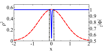
Figure 1: (Color online) Schematic representation of the regions of variation for each function. The “background solution” and the “soliton solution” are represented by dashed (red) and solid (blue) lines, respectively. Note that the left- and right-vertical curves in dash-dot (black) line delimit the region of variation of the two functions (approximately). While $\rho^{2}(x)$ varies on the outside, $|\Phi(x,0)|^{2}$ varies inside.

The result of Eq. (11) becomes exact for the limit cases $x\rightarrow\pm\infty$ ($\Phi_{\infty}$ constant) and $x\rightarrow 0$ (since the trap provides a background centered in $x=0$). Also, the Eq. (10) leads to a null result in these limit cases.

Now, defining $\mu=\lambda\sqrt{1+\sigma\rho_{0}^{2}|\Phi_{\infty}|^{2}}$ and assuming $R(\rho,\Phi)\simeq 0$ in (9), we will have

$$i\Phi_{t}+\mu\Phi=-\frac{1}{2}\Phi_{xx}+\lambda\sqrt{1+\sigma\rho_{0}^{2}|\Phi|^{2}}\Phi.$$ (12)

Next, using the rescaling $\Phi\equiv\widetilde{\Phi}/\rho_{0}$ one gets

$$i\widetilde{\Phi}_{t}+\mu\widetilde{\Phi}=-\frac{1}{2}\widetilde{\Phi}_{xx}+\lambda\sqrt{1+\sigma|\widetilde{\Phi}|^{2}}\widetilde{\Phi}.$$ (13)

Following, to solve the Eq. (13) we will use the ansatz

$$\widetilde{\Phi}=A(\zeta)e^{i\eta(\zeta)},$$ (14)

where $\zeta=x-vt$ with $v$ being the initial soliton velocity, and $A$ and $\eta$ are real functions. Inserting (14) in (13) we obtain the imaginary part satisfying

$$\eta_{\zeta}=v\left(1-\frac{A_{\infty}^{2}}{A^{2}}\right),$$ (15)

where $A_{\infty}$ is the value of $A(\zeta=\infty)$ and we have used $\lim_{\zeta\rightarrow\pm\infty}(\eta_{\zeta})=0$; the real part, considering the result of (15) evolves to

$$A_{\zeta\zeta}=-(v^{2}+2\mu)A+v^{2}\frac{A_{\infty}^{4}}{A^{3}}+2\lambda\sqrt{1+\sigma A^{2}}A.$$ (16)

The above equation can be reduced to a first order differential equation given by

$$A_{\zeta}=\pm\sqrt{2U+c_{1}},$$ (17)

where $U=-\frac{1}{2}(v^{2}+2\mu)A^{2}-(v^{2}A_{\infty}^{4}/2A^{2})+\frac{2\lambda}{3\sigma}(1+\sigma A^{2})^{3/2}$ and $c_{1}=2(v^{2}+\mu)A_{\infty}^{2}-\frac{4\lambda}{3\sigma}(1+\sigma A_{\infty}^{2})^{3/2}$, since we have consider $\lim_{\zeta\rightarrow\infty}(A_{\zeta})=0$. Now, considering $\lim_{\zeta\rightarrow\infty}(A_{\zeta\zeta})=0$ in Eq. (16) one obtains

$$A_{\infty}^{2}=\frac{1}{\sigma}\left(\frac{\mu^{2}}{\lambda^{2}}-1\right).$$ (18)

Note that for $A_{\infty}$ to be real one needs $\mu>\lambda$ ($\lambda$ is a positive constant as we had previously defined and $\sigma>0$). Also, the pattern of $U$ in (17) presents a local minimum corresponding to the value of $A_{\infty}$, such that $\left.U_{AA}\right|_{A_{\infty}}>0$ and consequently $\mu>v^{2}+\sqrt{v^{4}+\lambda^{2}}$. So, one gets a limit value for the chemical potential in function of the frequencies ratio $\lambda$ and the soliton velocity $v$.

Following, taken $\lim_{\zeta\rightarrow 0}\left(A^{2}\right)_{\zeta}=0$ in Eq. (17) we will obtain a quintic order equation in $A_{0}$, such that, by using the rescale $1+\sigma A_{0}^{2}\equiv\gamma^{2}$ one gets

$$a\gamma^{5}+b\gamma^{4}+c\gamma^{3}+d\gamma^{2}+e=0,$$ (19)

where $a=4\lambda^{5}$, $b=-3\lambda^{4}(v^{2}+2\mu)$, $c=-a$, $d=2\mu\lambda^{2}(3v^{2}\mu+3\lambda^{2}+\mu^{2})$, and $e=-\mu^{3}(3v^{2}\mu+2\lambda^{2})$. The Eq. (19) admit two solutions $\gamma=\gamma_{\infty}=\mu/\lambda$. In this case one can reduct the Eq. (19) for a third order equation given by $a^{\prime}\gamma^{3}+b^{\prime}\gamma^{2}+c^{\prime}\gamma+d^{\prime}=0$, with $a^{\prime}=4\lambda^{3}$, $b^{\prime}=\lambda^{2}(2\mu-3v^{2})$, $c^{\prime}=-2\lambda(3\mu v^{2}+2\lambda^{2})$, and $d^{\prime}=-\mu(3\mu v^{2}+2\lambda^{2})$. We have used the Cardano’s method to solve analytically this cubic equation. Indeed, the cubic equation has always one real positive root. We have used this root to get the value of $A_{0}$ and start a numerical method ($4^{th}$ order Runge-Kutta) to get the profiles of $A(\zeta)$ and $\eta(\zeta)$. So, Eq. (14) gives us the initial profile ($t=0$) of the homogeneous part of the ansatz (5). Note that the Eq. (5) takes the following form $\psi=f\widetilde{\Phi}/\rho_{0}|\Phi_{\infty}|$. Then, using our definition of $\mu$ we will have $\rho_{0}|\Phi_{\infty}|=\sqrt{(\mu/\lambda)^{2}-1}/\sqrt{\sigma}$ that is the transformation factor for the rescaled solutions. The last step consists in the use of $\psi(x,0)$ as the initial profile of the split-step algorithm to solve the Eq. (4).

IV Results

Next we will show the numerical results considering two different patterns of potential. In order to compare the results with the cubic case (Ref. ParkerPRA10 ), we will use here the expansion in first order

$$\lambda\sqrt{1+\sigma|\psi|^{2}}\simeq\lambda+(\lambda\sigma/2)|\psi|^{2}.$$ (20)

Note that in the cubic approximation the chemical potential is rescaled by $\lambda$, i.e., $\mu_{C}\equiv\mu-\lambda$, where $\mu_{C}$ ($\mu$) is the chemical potential for the cubic (nonpolynomial) case. Also, the cubic nonlinearity takes the corresponding relationship $\sigma_{C}=\lambda\sigma/2$. In the general case the two equalities above are not valid simultaneously due to the approximation (20). So, we will establish the equality between the nonlinearities, leaving aside the relationship between the chemical potentials to investigate in the next subsection the influence of a harmonic trap. We will name the cubic equation as 1D GP equation from now on.

IV.1 Harmonic trap

The standard case consists on the quadratic potential that confines the BEC

$$\overline{V_{x}}=x^{2}/2.$$ (21)

In this case a dark soliton (obtained following Eq. (5)) with an initial velocity at center of the BEC given by $v_{0}=0.5v_{l}$, where $v_{l}=\sqrt{\mu}$ and $v_{l}=\sqrt{\mu^{2}-\lambda^{2}}/\sqrt{2\mu}$ for the cubic and nonpolynomial case, respectively, evolves such that the velocity of dark soliton is reduced and the depth of the dark soliton is increased (reducing its velocity) until it touch the zero density. At this point, the velocity of the soliton changes its direction allowing an oscillatory pattern (like a particle in a harmonic oscillator). However, due to the soliton acceleration it emits a shock wave (sound wave). In the present case, the recombination soliton-sound maintains a stable solution.

Fig. 2(a) shows the renormalized density $|\psi|^{2}-f^{2}$ for the 1D GP equation as a function of time (similar results were verified for MMD). Sound waves are in light blur while the soliton position is in the dark trail. In Fig. 2(b) we display the temporal evolution of the soliton energy (see Appendix). The soliton position (as well as the mean position of the BEC, defined by $\overline{x}=\int_{-\infty}^{\infty}x|\psi|^{2}dx$) is coincident for both cases considering the parameters $\sigma_{C}=200$, $\sigma=2$ and $\lambda=200$. Note that the approximation (20) is more accurate for small values of $\sigma|\psi|^{2}$. So, the smaller $\sigma|\psi|^{2}$ is, since the relation $\sigma_{C}=\lambda\sigma/2$ is satisfied, better is the match for all calculated quantities comparing the results of the evolution in both models. This was confirmed in our numerical simulations. However, we stress that even considering the above relation between the nonlinearities, we need $\lambda\gg 1$ to be valid the 1D approximation.

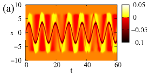
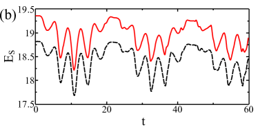
Figure 2: (Color online) Dark soliton dynamics in a harmonic trap. The renormalized density $|\psi|^{2}-f^{2}$ for the 1D GP equation are displayed in (a). The behavior of the dark soliton in the MMD equation is similar to the cubic case. (b) Soliton energy for the cubic in (red) solid line and nonpolynomial (black) dashed line, both in in units of $\hbar\omega_{z}\rho_{0}^{2}\xi$ (the dashed gray bars assist us to the visualization of the similar patterns). Here we have considered $v_{0}=0.5v_{l}$, where $v_{l}=\sqrt{\mu}$ and $v_{l}=\sqrt{\mu^{2}-\lambda^{2}}/\sqrt{2\mu}$ for the cubic and nonpolynomial case, respectively; $\sigma_{C}=200$, $\sigma=2$ and $\lambda=200$, providing $\mu_{C}\simeq 22.42$ (which is close to that used in Ref.ParkerPRA10 ) and $\mu-\lambda\simeq 21.76$.

In contrast with the above result, when considering $\sigma_{C}=2000$, $\sigma=100$ and $\lambda=40$, satisfying $\sigma_{C}=\lambda\sigma/2$, we have obtained a discrepant set of quantities. For example, the chemical potential is obtained to be $\mu_{C}=104$.00 and $\mu-\lambda=72.35$. Also, we have used the power spectrum of some functions to obtain the principal frequency contributions in these two cases. As expected, the oscillation frequency of the center of mass of the BEC is $\omega_{x}=1$ for the two cases. However, the oscillation frequencies for the solitonic position are $\omega_{C}\simeq 0.708$ and $\omega_{MMD}\simeq 0.72$. So, for the cubic case the relation $\omega_{x}/\omega_{C}=\sqrt{2}$ is satisfied while in the nonpolynomial case there is $2\%$ of error. This is also verified by using the energy oscillation.

Fig. 3(a) shows the input profiles for the two equations. Note that the solitonic profile seems similar but the background is more localized for the MMD equation. This evident contrast is verified in the energy scales displayed in Fig. 3(b) (left and right axis), as well as the difference between its oscillatory behaviors. The soliton positions for the two cases are shown in Fig. 3(c).

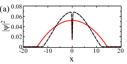
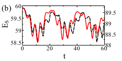
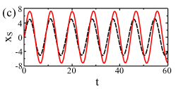
Figure 3: (Color online) Dark soliton dynamics in presence of an harmonic trap. (a) Input profiles. (b) Comparison between the energy values as function of time. Soliton energy values considering the MMD (GP) equation are displayed in left (right) axis. (c) Soliton position. The solid (red) lines represent the results for the GP equation while the results for the MMD equation is presented in dashed (black) lines. We have used $\sigma_{C}=2000$, $\sigma=100$ and $\lambda=40$.

IV.2 Gaussian trap

Here, we will consider a Gaussian trap of the form

$$\overline{V_{x}}=V_{0}\left[1-\exp\left(-x^{2}/2V_{0}\right)\right],$$ (22)

where $V_{0}$ is the depth of the trap. Firstly we want to know the influence of cutoff value $V_{0}$ to the soliton dynamics. To this end, we will fix a value for the nonlinearity in the 1D GP and MMD equations (namely, $\sigma_{C}=\lambda\sigma/2=1200$). Then, in this case the relation $\mu_{C}=\mu-\lambda$ will not be satisfied.

Since, by Thomas-Fermi approximation the BEC is concentrated in the region $\overline{V_{x}}<\mu-\lambda$, when $V_{0}<\mu-\lambda$ in (22), sound waves can scape of the trap. On the other hand, when $V_{0}\gg\mu-\lambda$, the sound waves are trapped and the potential is approximately harmonic in the BEC region.

These results are shown in Figs. 4(a) for $V_{0}=2\mu_{C}$ (trapped) and 4(b) for $V_{0}=\mu_{C}$ (sound escapes), considering the 1D GP equation. In Figs. 4(c) and 4(d) we display the rescaled soliton profile for the MMD equation considering $V_{0}=2\mu_{C}$ and $V_{0}=\mu_{C}$, respectively. Note that for $V_{0}=\mu_{C}$ ($\mu_{C}\simeq 61.19$) the sound escapes in the 1D GP equation but it does not escapes in the MMD equation. This is evident once we have abdicated to the equality for the chemical potential and its correct value in the MMD equation is to be $\mu-\lambda\simeq 51.29$ when we set $\sigma=40$ and $\lambda=60$, satisfying the relation $\sigma_{C}=\lambda\sigma/2$.

The temporal evolution of the rescaled soliton energies are shown in Figs. 4(e) and 4(f) for $V_{0}=2\mu_{C}$ and $V_{0}=\mu_{C}$, respectively. The results for the 1D GP equation are displayed in solid (black) lines while dashed (red) lines represent the MMD equation. It is clear by Fig. 4(f) the dissipative behavior when considering the cubic nonlinearity in opposition to the trapped form when the nonlinearity is nonpolynomial. For the latter, the soliton-sound recombination destroys the soliton faster than the dissipative case given by 1D GP equation. Also, in Fig. 4(e) one can see that the soliton lifetime is different in both cases, i.e., $t=235.8$ ($t\simeq 6.4$s) for the cubic case and $t>300$ ($t\gtrsim 8$s) for the nonpolynomial case.

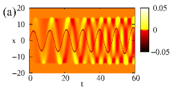
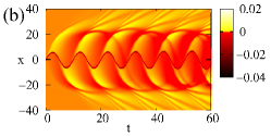
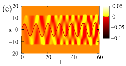
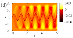
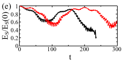
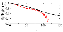
Figure 4: (Color online) Renormalized density profile of dark soliton ($|\psi|^{2}-f^{2}$) for the cubic (a) and (b) and nonpolynomial nonlinearity (c) and (d). We have used $\sigma_{C}=\lambda\sigma/2=1200$ ($\sigma=40$ and $\lambda=60$) with $V_{0}=2\mu_{C}$ in (a) and (c) and $V_{0}=\mu_{C}$ in (b) and (d). Evolution of the renormalized soliton energy $E_{S}/E_{s}(t=0)$ in a Gaussian trap for (e) $V_{0}=2\mu_{C}$ and (f) $V_{0}=\mu_{C}$. The results of the 1D GP and MMD equations are displayed in solid (black) and dashed (red) lines, respectively.

To verify the influence of $\lambda$ in the soliton-sound recombination we display in Fig. 5 the temporal evolution of the soliton energy $E_{S}$ for the nonpolynomial case, considering $\lambda=200$ in solid (black) line, $\lambda=100$ in dashed (red) line, and $\lambda=50$ in doted (green) line. We have used the gaussian depth $V_{0}=2(\mu-\lambda)$, with $\mu-\lambda=21.76$. Note that decreasing the value of $\lambda$ the lifetime of the soliton is increased. When $\lambda=200$, $\lambda=100$, and $\lambda=50$ the corresponding soliton lifetimes are $t\simeq 47.7\omega_{x}^{-1}$, $t\simeq 49.6\omega_{x}^{-1}$, and $t\simeq 54.1\omega_{x}^{-1}$, respectively. This accounts a difference of $\sim 13\%$ comparing the lifetime of the first and last cases.

We now attempt to the experimental parameters obtained in Ref. BeckerNP08 . In BeckerNP08 $\omega_{x}=2\pi\times 5.9\mathrm{Hz}$ and $\omega_{\perp}\sim 2\pi\times 109\mathrm{Hz}$, which leads to $\lambda\simeq 18.5$. The chemical potential is $\mu_{C}/k_{B}\simeq 20$ nK, where $k_{B}$ is the Boltzmann constant. In this case, one can estimate $\mu_{C}\simeq 70.6$ and consequently $\sigma_{C}\simeq 1136.02$ by using the relation $\mu_{C}=\sigma_{C}n_{0}$ with $n_{0}$ obtained through the profile obtained by propagation in imaginary time of the 1D GP equation with $V_{0}\gg\mu_{C}$ ($V_{0}=10\mu_{C}$). Following, using $\sigma_{C}$ and $\lambda$ given above we obtain numerically $\mu\simeq 63.4$ (for $V_{0}=10(\mu-\lambda)$).

Next, by using the value of $\mu_{C}$ given above we estimate using the profile obtained via the imaginary time propagation for the cubic equation ($V_{0}\gg\mu_{C}$), a density peak for the background and consequently the non-linearity intensity given by $\rho_{0}^{2}\simeq 6.2\times 10^{-2}$ and $\sigma_{C}\simeq 1118.5$, respectively. Also, through $\mu$ above, we obtain $\rho_{0}^{2}\simeq 8.3\times 10^{-2}$ and $\sigma\simeq 163.2$.

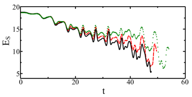
Figure 5: (Color online) Temporal evolution of the soliton energy $E_{S}$ for a Gaussian trap with cutoff $V_{0}=2(\mu-\lambda)$. Solid (black) line corresponds to $\lambda=200$, in dashed (red) line $\lambda=100$, and in doted (green) line $\lambda=50$. For all cases we have used $\mu-\lambda=21.76$.

V Conclusion

In conclusion, we have studied the soliton-sound interaction in the MMD equation, which is an effective 1D equation governing the axial dynamics of a cigar-shaped BEC with repulsive interatomic interactions, accounting accurately for the contribution from the transverse degrees of freedom. A significant differences has been observed when comparing the soliton dynamics in MMD and 1D GP equation. In particular, increasing the strength of the repulsive interatomic interaction the divergence between the results appears naturally. Also, the soliton-sound recombination presents an important hole in the lifetime of dark solitons, as shown in the literature ParkerJPB04 ; ParkerPRA10 ; ParkerPRL03 . When the perfect recombination does not occurs, for example in anharmonic traps like that presented here, the soliton can scape from the trap or simply to decay. This is in agreement with the results obtained in the present paper. We believe that this can motivate further investigations of soliton- or vortex-sound interactions in realistic systems with more dimensions.

Appendix: Dark soliton energy

In presence of a confining potential the energy of the solution is a finite constant. However, we want to compute only the contribution of the dark soliton energy. To this end, we will use the renormalized energy density, given by Kivshar03

$$\epsilon(\psi)=\frac{1}{2}|\psi_{x}|^{2}+\overline{V}|\psi|^{2}+\int_{f_{0}^{2}}^{|\psi|^{2}}[F(I)-F(f_{0}^{2})]dI,$$ (23)

where $F(I)=\sigma_{C}I$ and $F(I)=\lambda\sqrt{1+\sigma I}$ for the cubic and nonpolynomial NLS equation, respectively. In the case of cubic nonlinearity the Eq. (23) reduces to a similar form of Eq. (A2) of Ref. ParkerPRA10 . Next we will use the following definition for the soliton energy

$$E_{s}=\int_{x_{s}-x_{int}}^{x_{s}+x_{int}}\epsilon(\psi)dx-\int_{x_{s}-x_{int}}^{x_{s}+x_{int}}\epsilon(f)dx,$$ (24)

where $f$ is the time-independent background density in the absence of the soliton (i.e., the solution from the imaginary time propagation of the Eq.(8)) and $f_{0}$ denotes the peak condensate density at the center of the trap for purely harmonic confinement. Here, $x_{s}$ is the soliton position and $x_{int}$ is the domain of integration around the soliton position. To find $x_{int}$ we have varied its value until $E_{s}$ does not change anymore (we have stopped the variation of $x_{int}$ with a difference of energy of the order of $10^{-14}$). This value is compared to that obtained in Ref. ParkerPRA10 .

References

- (1) Y. S. Kivshar and G. P. Agrawal, Optical Solitons: From Fibers to Photonic Crystals (Academic Press, San Diego, USA, 2003).
- (2) D. Krökel, N. J. Halas, G. Giuliani, and D. Grischkowsky, Phys. Rev. Lett. 60, 29 (1988); G. A. Swartzlander, D. R. Andersen, J. J. Regan, H. Yin, and A. E. Kaplan, ibid. 66, 1583 (1991).
- (3) B. Denardo, W. Wright, S. Putterman, and A. Larraza, Phys. Rev. Lett. 64, 1518 (1990).
- (4) M. Chen, M. A. Tsankov, J. M. Nash, and C. E. Patton, Phys. Rev. Lett. 70, 1707 (1993).
- (5) S. Burger, S. Dettmer, W. Ertmer, K. Sengstock, A. Sanpera, G. V. Shlyapnikov, and M. Lewenstein, Phys. Rev. Lett. 83, 5198 (1999).
- (6) J. Denschlag, J. E. Simsarian, D. L. Feder, C. W. Clark, L. A. Collins, J. Cubizolles, L. Deng, E. W. Hagley, K. Helmerson, W. P. Reinhart, S. L. Rolston, B. I. Schneider, and W. D. Phillips, Science 287, 97 (2000).
- (7) B. P. Anderson, P. C. Haljan, C. A. Regal, D. L. Feder, L. A. Collins, C. W. Clark, and E. A. Cornell, Phys. Rev. Lett. 86, 2926 (2001).
- (8) Z. Dutton, M. Budde, C. Slowe, and L.V. Hau, Science 293, 663 (2001).
- (9) W. P. Reinhardt and C. W. Clark, J. Phys. B 30, L785 (1997).
- (10) T. F. Scott, R. J. Ballagh, and K. Burnett, J. Phys. B 31, L329 (1998).
- (11) Th. Busch and J. R. Anglin, Phys. Rev. Lett. 84, 2298 (2000).
- (12) G. Huang, J. Szeftel, and S. Zhu, Phys. Rev. A 65, 053605 (2002).
- (13) N. G. Parker, N. P. Proukakis, and C. S. Adams, Phys. Rev. A 81, 033606 (2010).
- (14) N. G. Parker, N. P. Proukakis, M. Leadbeater, and C. S. Adams, Phys. Rev. Lett. 90, 220401 (2003).
- (15) N. P. Proukakis, N. G. Parker, C. F. Barenghi, and C. S. Adams, Phys. Rev. Lett. 93, 130408 (2004).
- (16) A. Muñoz-Mateo and V. Delgado, Phys. Rev. A 77, 013617 (2008).
- (17) A. M. Mateo and V. Delgado, Phys. Rev. A 75, 063610 (2007); A. Muñoz-Mateo and V. Delgado, ibid. 74, 065602 (2006).
- (18) C. J. Pethick and H. Smith, Bose-Einstein Condensation in Dilute Gases (Cambridge University Press, Cambridge, 2002); L. Pitaevskii and S. Stringari, Bose-Einstein Condensation (Clarendon Press, Oxford, 2003).
- (19) N. G. Parker, N. P. Proukakis, C. F. Barenghi, and C. S. Adams, J. Phys. B: At. Mol. Opt. Phys. 37, S175 (2004).
- (20) A. Muryshev, G. V. Shlyapnikov, W. Ertmer, K. Sengstock, and M. Lewenstein, Phys. Rev. Lett. 89, 110401 (2002).
- (21) V. A. Brazhnyi and V. V. Konotop, Phys. Rev. A 68, 043613 (2003).
- (22) L. Salasnich, A. Parola, and L. Reatto, Phys. Rev. A 69, 045601 (2004).
- (23) J. Yang, Nonlinear Waves in Integrable and Nonintegrable Systems (Society for Industrial and Applied Mathematics SIAM, Philadelphia, 2010).
- (24) P. Muruganandam and S. K. Adhikari, Comput Phys. Commun 180, 1888 (2009).
- (25) C. Becker et al., Nature Phys. 4, 496 (2008).