The UM, a fully–compressible, non–hydrostatic, deep atmosphere GCM, applied to hot Jupiters.

We are adapting the Global Circulation Model (GCM) of the UK Met Office, the so–called Unified Model (UM), for the study of hot Jupiters. In this work we demonstrate the successful adaptation of the most sophisticated dynamical core, the component of the GCM which solves the equations of motion for the atmosphere, available within the UM, ENDGame (Even Newer Dynamics for General atmospheric modelling of the environment). Within the same numerical scheme ENDGame supports solution to the dynamical equations under varying degrees of simplification. We present results from a simple, shallow (in atmospheric domain) hot Jupiter model (SHJ), and a more realistic (with a deeper atmosphere) HD 209458b test case. For both test cases we find that the large–scale, time–averaged (over the 1200 days prescribed test period), dynamical state of the atmosphere is relatively insensitive to the level of simplification of the dynamical equations. However, problems exist when attempting to reproduce the results for these test cases derived from other models. For the SHJ case the lower (and upper) boundary intersects the dominant dynamical features of the atmosphere meaning the results are heavily dependent on the boundary conditions. For the HD 209458b test case, when using the more complete dynamical models, the atmosphere is still clearly evolving after 1200 days, and in a transient state. Solving the complete (deep atmosphere and non–hydrostatic) dynamical equations allows exchange between the vertical and horizontal momentum of the atmosphere, via Coriolis and metric terms. Subsequently, interaction between the upper atmosphere and the deeper more slowly evolving (radiatively inactive) atmosphere significantly alters the results, and acts over timescales longer than 1200 days.

1 Introduction

Observations made over the last 20 years have enabled the detection of several hundred exoplanets (the first around a Solar mass star by Mayor & Queloz, 1995) and several thousand candidate systems (identified, for instance, by the Kepler mission including the discovery of a system of six planets and a sub–Mercury sized planet, see Lissauer et al., 2011; Barclay et al., 2013, respectively). Surveys of variability (detecting planetary transits) and radial velocity have also provided estimates of the mass and orbital radii of these exoplanets. Such surveys are most sensitive to giant ($\sim$Jovian mass) planets which orbit close to their parent stars, experience intense radiation ($10^{3}-10^{5}$ times that received by Jupiter, exacerbating problems involved with simplified radiative transfer schemes), and are termed ‘hot Jupiters’. The strong tidal forces experienced by these planets is thought to lead to rapid synchronisation of their rotation period with their orbital period (with the adoption of a reasonable dissipation parameter). This ‘tidal–locking’ provides a strong constraint on the planetary rotation rate and means the planet has a permanent day and night side, experiencing net heating and cooling, respectively (see Baraffe et al., 2010, and references therein).

Furthermore, precise observations of the luminosity as a function of time and wavelength (transit spectroscopy) of a transiting star–planet system can be used to probe the planet’s atmospheric conditions (see Seager & Deming, 2010, for review). Observations of the primary eclipse (when the planet transits in front of the star) have provided the detection of specific species in the atmospheres of hot Jupiters (see for example Sing et al., 2011, 2012, who detected potassium and sodium, respectively, in the atmosphere of Xo–2b) as well as the detection of possible dust or hazes (for example as found in HD 189733b, Pont et al., 2012). Additionally observations of both the primary and secondary eclipses (when the planet moves behind the star) have allowed the derivation of day and night side atmospheric temperatures (for example $\sim$1250 K and $\sim$1000 K for HD 189733b as found by Knutson et al., 2007, 2009). Moreover, using the full orbital luminosity phase–curve, the atmospheric temperature as a function of planetary longitude can be inferred (see for example Knutson et al., 2007, 2009). Analysis of these temperature ‘maps’ has revealed offsets of the hottest part of the atmosphere or ‘hot spot’ (at a given depth) from the sub-stellar points. This offset was predicted by Showman & Guillot (2002) as a consequence of the expected fast circulations induced by the large–scale heating. The presence of such fast winds has been suggested for HD 209458b using Doppler shifting of molecular CO bands (Snellen et al., 2010), where $\sim$km s^-1 wind speeds were derived.

Although this is not a complete review of the observational results, the observations have produced several challenges for our theoretical models of planetary evolution. Many of these challenges require an understanding of the full three dimensional circulation, including the vertical transport. Firstly, comparison of the derived radii with the predictions of planetary interior models (as a function of age) has shown that some hot Jupiters appear inflated. Guillot & Showman (2002) suggested that the vertical transport of $\sim 1$ percent of the incident stellar flux, from the top of the atmosphere deep into the planet interior, could halt the planet’s gravitational contraction sufficiently to explain the observations. Showman & Guillot (2002) then suggested that the required levels of kinetic energy could be generated by the large–scale forcing expected in hot Jupiter atmospheres. Secondly, as is evident for Solar system planets, significant abundances of scattering particles can dominate the global heat balance of a planet’s atmosphere (see for discussion Sánchez-Lavega et al., 2004), which is difficult to capture using simplistic radiative transfer schemes.

The possible presence of scattering particles (suggested to be MgSiO₃ by Lecavelier Des Etangs et al., 2008) in the observable atmospheres of hot Jupiters requires they be supported against gravitational settling and/or be replenished via circulations. Therefore, vertical transport modeled over a large range of pressures is vital to interpreting these observations, in addition to a non-grey radiative transfer scheme. Finally, comparison of day and night side temperatures has revealed a possible dichotomy separating hot Jupiters with efficient heat redistribution (from day to night side), which are generally more intensely irradiated, from those exhibiting less efficient heat redistribution. The efficiency of redistribution has been linked to the existence of a region of the hot Jupiter upper atmosphere where temperature increases with height, a thermal inversion, as inferred from model fitting for HD 209458b (Knutson et al., 2008), and thereby the presence of absorbing substances such as VO and TiO (Hubeny et al., 2003; Fortney et al., 2008). A correct description of all these processes requires a non–grey radiative transfer scheme coupled to a dynamical model of the atmospheric redistribution.

The glimpses into the atmospheres of hot Jupiters provided by the observations, and the associated puzzles, have motivated the application of Global Circulation Models (GCMs), usually developed for the study of Earth’s weather and climate, to hot Jupiters. GCMs are generally comprised of many components or modules which handle different aspects of the atmosphere. Many of these components are highly optimised for conditions on Earth, for example treatments of the surface boundary layer. To apply GCMs to planets other than Earth adaptation of the most fundamental components i.e. treating radiative transfer and dynamical motions, is required. Further adaptations to more detailed atmospheric process can then occur when merited by observations.

GCMs have been successfully applied to model other Solar system planets (see for example models of Jupiter, Saturn, Mars and Venus: Yamazaki et al., 2004; Müller-Wodarg et al., 2006; Hollingsworth & Kahre, 2010; Lebonnois et al., 2011, respectively), but hot Jupiters present a very different regime. The latter receive significantly more radiation and rotate much more slowly than the giant planets in our Solar system. Therefore, the characteristic scales of atmospheric features such as the expected vortex size, the Rossby deformation radius and the elongation in the east–west direction of wind structures, the Rhines scale are both approximately the size of the planet (proportionally much larger than for Solar system planets, see Showman et al., 2011, for a review and comparison with Solar system planets). This effectively means that one might expect any ‘weather systems’, or jet structures (i.e. prevailing circumplanetary flows) to be comparable in size with the horizontal extent of the atmosphere. Despite the exotic nature of the flow regime, the adaptation of GCMs to hot Jupiters has met with success as, for example, several models have been able to demonstrate that offsets in the ‘hot spot’ are consistent with redistribution from zonal (longitudinal direction) winds (Showman et al., 2009; Dobbs-Dixon & Lin, 2008; Dobbs-Dixon, 2009). The progress of the modelling has been reviewed in Showman et al. (2008, 2011) and a useful summary of the different approaches taken can be found in Dobbs-Dixon & Agol (2012).

To interpret the observations of hot Jupiters the regime dictates the model should include solution to the full three–dimensional equations of motion for a rotating atmosphere coupled to a non–grey radiative transfer scheme. This will allow exploration of the consequences of realistic vertical transport and its interaction with the horizontal advection, and include the effect on the thermal balance of the atmosphere caused by frequency dependent opacities. Most GCMs applied to hot Jupiters solve the primitive equations of meteorology, involving the approximation of vertical hydrostatic equilibrium, and a ‘shallow–atmosphere’ (combining the constant gravity, ‘shallow–fluid’ and ‘traditional’ approximations, see Vallis, 2006; White et al., 2005).

The most sophisticated radiative transfer scheme within a GCM, applied to hot Jupiters, to date is that of Showman et al. (2009) which solves the primitive equations coupled to a simplified radiative transfer scheme based on the two-stream, correlated–$k$ method. However, the approximations involved in the primitive equations neglect the vertical acceleration of fluid parcels, and the effect of the vertical velocity on the horizontal momentum. More complete dynamical models, solving the full Navier–Stokes equations, have been applied to hot Jupiters by Dobbs-Dixon & Lin (2008); Dobbs-Dixon (2009); Dobbs-Dixon et al. (2010); Dobbs-Dixon & Agol (2012), but these models include a radiative transfer scheme more simplified than the method of Showman et al. (2009). Dobbs-Dixon et al. (2010) includes frequency dependent radiative transfer via the introduction of only three opacity bins (and generally runs for short elapsed model times). Dobbs-Dixon & Agol (2012) includes a treatment using a similar number of frequency bins to Showman et al. (2009), but simply average the opacity in each bin as opposed to generating opacities via the correlated–k method.

Therefore, calculations based on non–grey radiative transfer coupled to full three–dimensional equations of motion for a rotating atmosphere do not yet exist. Additionally, current models applied to hot Jupiters are still missing many other physical processes. Although not discussed in this paper, treatments of the magnetic fields, photochemistry and clouds or hazes, may well be required to create a model capable of meaningful predictions. We are beginning work on the incorporation of a photochemical network and the simple modelling of clouds into our model, but this will take some time to complete.

The ENDGame (Even Newer Dynamics for General atmospheric modelling of the environment) dynamical core (the part of the GCM solving the discretised fluid dynamics equations of motion) of the UK Met Office GCM, the Unified Model (UM) is based on the non–hydrostatic deep–atmosphere equations (Staniforth & Wood, 2003, 2008; Wood et al., 2013), and does not make the approximations incorporated in the primitive equations (White et al., 2005). The UM also includes a two–stream radiative transfer scheme with correlated–k method. This code has previously been adapted to studies of Jupiter (Yamazaki et al., 2004), but requires significant adaptation of the dynamical and radiative transfer schemes to be applied to hot Jupiters. We have previously presented the satisfactory completion of several Earth–like test cases of the dynamical core in Mayne et al. (2013). Now, we have completed the adaptation of the dynamical core, and in this work present the first hot Jupiter test cases. We have completed the Shallow–Hot Jupiter (SHJ, as prescribed in Menou & Rauscher, 2009) and the HD 209458b test case of Heng et al. (2011).

Adaptation of the radiative transfer scheme is nearing completion and coupled models will be presented in a future work. With this paper, we begin a series in which we will present the details of the model developments and testing of the UM, as it is adapted for the study of exoplanets, as well as scientific applications and results.

The structure of the paper is as follows. In Section 2 we detail the model used including the equations solved and highlight the important details of our boundary conditions and numerical scheme. We also discuss the effect of canonical simplifications made to the dynamical equations. Section 2 also includes an explanation of the parameterisations used and references to a more detailed description of the model and previous testing. Section 3 then describes the setups for two test cases we have run including the parameter values and temperature and pressure profiles. We also, in Section 3 demonstrate satisfactory completion of these tests. Section 4 highlights some problems with the test cases and discusses future work. Finally, in Section 5 we include a summary of our conclusions.

2 Model

The UM dynamical core called ENDGame is explained in detail in Wood et al. (2013). The code is based on the non–hydrostatic, deep–atmosphere (NHD) equations of motion for a planetary atmosphere (Staniforth & Wood, 2003, 2008), including a varying (with height) gravity and a geometric height vertical grid. Uniquely, the code allows solution to the non–hydrostatic shallow–atmosphere (NHS, Staniforth & Wood, 2003, 2008) equations, or just the simple assumption of a constant gravity (to create a quasi–NHD system), within the same numerical scheme.

2.1 Overview of the numerical scheme

The UM is a finite–difference code where the atmosphere is discretised onto a latitude–longitude grid (resolutions explained in Section 3), using a staggered Arakawa–C grid (Arakawa & Lamb, 1977) and a vertically staggered Charney–Phillips grid (Charney & Phillips, 1953). The code uses a terrain following height–based vertical coordinate.

The code is semi–Lagrangian and semi–implicit, where the latter is based on a Crank–Nicolson scheme. The code employs semi–Lagrangian advection where the values for advected quantities are derived at interpolated departure points, and are then used to calculate quantities within the Eulerian grid. For the semi–implicit scheme the temporal weighting between the $i$th and the $i+1$th state is set by the coefficient $\alpha$ which can vary between zero and one, and is set to 0.55 in this work. For each atmospheric timestep a nested iteration structure is used. The outer iteration performs the semi–Lagrangian advection (including calculation of the departure points), and values of the pressure increments from the inner iteration are back substituted to obtain updated values for each prognostic variable. The inner iteration solves the Helmholtz (elliptical) problem to obtain the pressure increments, and the Coriolis and nonlinear terms are updated.

The velocity components are staggered such that the meridional velocity is defined at the pole (see Mayne et al., 2013, for a more detailed explanation), but no other variable is stored at this location, thereby avoiding the need to solve for pressure at the poles of the latitude–longitude grid (Wood et al., 2013). Thuburn & Staniforth (2004) show that mass, angular momentum and energy are much more readily conserved with a grid staggered such that $v$ and not $u$ is held at the pole. The stability afforded by the spatial and temporal discretisation removes the need for an explicit polar filter (although our diffusion operator has some aspects in common with a polar filter, see discussion in Section 2.6). The code adopts SI units. A full description of the code can be found in Wood et al. (2013) and important features relating to the reproduction of idealised tests are reiterated in Mayne et al. (2013).

2.2 Previous Testing

The UM undergoes regular verification for the Earth system, and Wood et al. (2013) completes several tests from the Dynamical Core Model Intercomparison Project, and the deep–atmosphere baroclinic instability test (Ullrich et al., 2013), using the ENDGame dynamical core. We have also, as part of the adaptation to exoplanets completed several tests for an Earth–like model including the Held-Suarez test (Held & Suarez, 1994), the Earth-like test of Menou & Rauscher (2009) and the Tidally Locked Earth of Merlis & Schneider (2010), the results of which are presented in Mayne et al. (2013). Additionally, for each setup used we also complete a static, non–rotating, hydrostatic isothermal atmosphere test, ensuring that the horizontal and vertical velocities recorded are negligibly small and do not grow significantly with time (when run for a few million iterations).

For simulations we have performed, the longest of which is many millions of iterations, mass and angular momentum, are conserved to better than $\lesssim 0.05$% and $\sim 5$%, respectively. In the UM mass is conserved via a correction factor applied after each timestep (see Wood et al., 2013, for details).

2.3 Equations solved by the dynamical core

We model only a section, or spherical shell, of the total atmosphere and define the material below our inner boundary (discussed in more detail in Section 2.4) as the ‘planet’ and the subscript ${\rm p}$ denotes quantities assigned to this region. The dynamical core solves a set of five equations: one for each momentum component, a continuity equation for mass and a thermodynamical energy equation, which are closed by the ideal gas equation. These equations are (using the “Full” equation set, see Table 1 for explanation)

$$\frac{Du}{Dt}=\frac{uv\tan\phi}{r}-\frac{uw}{r}+fv-f^{\prime}w-\frac{c_{p}\theta}{r\cos\phi}\frac{\partial\Pi}{\partial\lambda}+\textbf{D}(u),$$ (1)

$$\frac{Dv}{Dt}=-\frac{u^{2}\tan\phi}{r}-\frac{vw}{r}-uf-\frac{c_{p}\theta}{r}\frac{\partial\Pi}{\partial\phi}+\textbf{D}(v),$$ (2)

$$\delta\frac{Dw}{Dt}=\frac{u^{2}+v^{2}}{r}+uf^{\prime}-g(r)-c_{p}\theta\frac{\partial\Pi}{\partial r},$$ (3)

$$\frac{D\rho}{Dt}=-\rho\left[\frac{1}{r\cos\phi}\frac{\partial u}{\partial\lambda}\right.+\frac{1}{r\cos\phi}\frac{\partial(v\cos\phi)}{\partial\phi}\left.+\frac{1}{r^{2}}\frac{\partial(r^{2}w)}{\partial r}\right],$$ (4)

$$\frac{D\theta}{Dt}=\frac{Q}{\Pi}+\textbf{D}(\theta),$$ (5)

$$\Pi^{\frac{1-\kappa}{\kappa}}=\frac{R\rho\theta}{p_{0}},$$ (6)

respectively. The coordinates used are $\lambda$, $\phi$, $r$ and $t$, which are the longitude, latitude (from equator to poles), radial distance from the centre of the planet and time. The spatial directions, $\lambda$, $\phi$ and $r$, then have associated wind components $u$ (zonal), $v$ (meridional) and $w$ (vertical). $c_{p}$ is the specific heat capacity, $R$ is the gas constant and $\kappa$ the ratio of the $R/c_{p}$. $\delta$ is a ‘switch’ (0 or 1) to enable a quasi–hydrostatic version of the equations (not used in this work but detailed in White et al., 2005). $p_{0}$ is a chosen reference pressure and $g(r)$ is the acceleration due to gravity at $(r)$ and is defined as

$$g(r)=g_{\rm p}\left(\frac{R_{\rm p}}{r}\right)^{2},$$ (7)

where $g_{\rm p}$ and $R_{\rm p}$ are the gravitational acceleration and radial position at the inner boundary. $f$ and $f^{\prime}$ are the Coriolis parameters defined as,

$$f=2\Omega\sin\phi,$$ (8)

and

$$f^{\prime}=2\Omega\cos\phi,$$ (9)

where $\Omega$ is the planetary rotation rate. $\rho$ and $\theta$ are the prognostic variables of density and potential temperature, respectively. $\Pi$ is the Exner pressure (or function). $\theta$ and $\Pi$ are then defined, in terms of the temperature, $T$ and pressure, $p$, as

$$\theta=T\left(\frac{p_{0}}{p}\right)^{\frac{R}{c_{p}}},\\$$ (10)

and

$$\Pi=\left(\frac{p}{p_{0}}\right)^{R/c_{p}}=\frac{T}{\theta},\\$$ (11)

respectively. The material derivative, $\frac{D}{Dt}$ is given by

$$\frac{D}{Dt}=\frac{\partial}{\partial t}+\frac{u}{r\cos\phi}\frac{\partial}{\partial\lambda}+\frac{v}{r}\frac{\partial}{\partial\phi}+w\frac{\partial}{\partial r}.\\$$ (12)

Finally, $Q$ and D are the heating rate and diffusion operator (note that diffusion is not applied to the vertical velocity), respectively. The heating, in this work, is applied using a temperature relaxation or Newtonian cooling scheme discussed in Section 2.7. The diffusion operator is detailed in Section 2.6.

2.3.1 Dynamical simplification and variants of the equations of motion

A quartet of self–consistent governing dynamical equations conserving axial angular momentum, energy and potential vorticity are described in detail in White et al. (2005). These are the hydrostatic primitive equations or (hydrostatic) primitive equations (HPEs), quasi–hydrostatic equations (QHEs), the non–hydrostatic shallow–atmosphere (NHS) equations and the non–hydrostatic deep–atmosphere (NHD) equations. For this work we, using ENDGame, solve the NHD (which are detailed in Section 2.3), the quasi–NHD (with a constant gravity) and the NHS equations. White et al. (2005) includes a full discussion of the assumptions made in each equation set, the most relevant (for this work) of which are included in Table 1 alongside the validity criteria, and an estimate for the validity on HD 209458b (an example hot Jupiter).

Table 1 also includes the short reference names we have used to describe each setup. We adopt the nomenclature of White et al. (2005), where the ‘shallow–atmosphere’ approximation implies constant gravity, in addition to the adoption of the ‘shallow–fluid’ and ‘traditional’ approximations. In this work we run simulations using the “Full” (NHD), “Deep” (quasi–NHD i.e. constant gravity) and “Shallow” (NHS) equations sets, where the primitive equations (HPEs) are included as illustrative of the codes we compare against. However, the GCMs we are comparing with use either pressure or $\sigma$ ($=p/p_{\rm surf}$, where $p_{\rm surf}$ is the pressure at the inner boundary, which is usually called the “surface” for terrestrial planets) as their vertical coordinate. The key point is that when we compare models using for instance the “Shallow” equations with the primitive equations, we are simply relaxing the assumption of hydrostatic equilibrium. Moving to the “Deep” equations then involves further relaxing the ‘shallow–fluid’ and ‘traditional’ approximation (but retaining a constant gravity) and finally, the “Full” equations include a further relaxation of the constant gravity approximation.

Table 1: Key assumptions in each equation set, the local name used to describe the set, and the validity, both in general and for HD 209458b. $\Phi$ and $G$ are the geopotential and gravitational constant respectively. $M_{\rm p}$ and $M_{\rm atm}$ are the total masses of the planet below the inner boundary, and of the atmosphere, respectively. $z$ is the vertical height from the inner boundary. $H$ and $L$ are the vertical and horizontal sizes of the atmospheric domain. Finally, $N$ is the buoyancy (or Brunt-Väisälä) frequency, $N=\sqrt{-\frac{g(r)}{\rho_{0}}\frac{\partial\rho(r)}{\partial r}}$). SI units are used unless otherwise stated.

Name				Approximation		Formal Condition	HD 209458b
Primitive{70mm[]	Shallow{60mm[]	Deep{30mm[]	Full{20mm[]	Spherical geopotentials(1)	$\Phi(\lambda,\phi,r)=\Phi(r)$	$\Omega^{2}r\ll g$(2)	$10^{-2}\ll 10^{1}$
				no self-gravity	$g(r)=\frac{GM_{\rm p}}{r^{2}}$	$M_{\rm atm}\ll M_{\rm p}$	$\sim 10^{23}\ll 10^{27}$
				constant gravity	$g(r)=g_{\rm p}=\frac{GM_{\rm p}}{R_{\rm p}^{2}}$	$z\ll R_{\rm p}$	{24mm[]$\sim 10^{7}<10^{8}$
				‘shallow–fluid’	$r\rightarrow R_{\rm p}$ & $\frac{\partial}{\partial r}\rightarrow\frac{\partial}{\partial z}$	$z\ll R_{\rm p}$
				‘traditional’	$\frac{uw}{r}$, $\frac{vw}{r}$, $2\Omega w\cos\phi$ $\rightarrow 0$	$N^{2}\gg\Omega^{2}$(3)	$\sim 10^{-5}\gg 10^{-10}$
					$\frac{u^{2}+v^{2}}{r}$, $2\Omega u\cos\phi$ $\rightarrow 0$
				hydrostasy	$\frac{\partial\Pi}{\partial r}=-\frac{g}{c_{p}\theta}$ or $\frac{\partial p}{\partial r}=-\rho g$	$H\ll L$	$\sim 10^{7}<10^{8}$

(1) For a full discussion on the impact of the spherical geopotentials approximation see White et al. (2008). (2) This condition neglects tidal deformation, essentially assuming the planetary gravitational field is well isolated (see discussion in text). (3) Condition from Phillips (1968), but may not be sufficient (see discussion in White & Bromley, 1995).

The assumptions pertaining to gravity require some explanation. Firstly, the gravitational potential of the planet is assumed to be well isolated from external gravity fields (this is not the case in some hot Jupiters, for instance Wasp–12, Li et al., 2010). Secondly, care must be taken over how to solve for the centrifugal force, and subsequently construct the gravitational potential.

When modelling the Earth the acceleration due to gravity can be measured at the surface, $g_{\rm p}$. This is in effect the acceleration due to the apparent gravity as it includes contributions from both the gravitational and centrifugal components . This combined gravitational and centrifugal potential, or geopotential is then, in most cases, assumed to be spherically symmetric. This means, however, that the divergence of the resulting combined potential is not zero, as should be the case (see White et al., 2008, for a detailed discussion of the spherical geopotentials approximation). Additionally, this spurious divergence in the combined potential is increased if one adopts a constant gravitational acceleration throughout the atmosphere, as opposed to allowing it to fall via an inverse square law (White & Wood, 2012).

Calculating the acceleration due to the gravitational potential only, and solving explicitly, as part of the dynamical equations, for the centrifugal component, however, introduces spurious motions. For example a modeled hydrostatically balanced and statically stable atmosphere, at rest, would subsequently have to adjust to the apparent gravity caused by the rotation, which generates a horizontal force, creating winds.

For hot Jupiters the acceleration due to gravity cannot be measured, and there is no surface, in the same sense as on Earth or any other terrestrial planet. Therefore a value for $g_{\rm p}$ must be estimated using measurements of the total mass of the planet, $M_{\rm p}$ (derived from radial velocity measurements), and assuming this to be contained within a radius, $R_{\rm p}$ (practically the smallest available radius derived from observations of the primary eclipse). The precision to which $g_{\rm p}$ is estimated, or quoted, is much lower than the magnitude of the expected effect of the centrifugal component. Therefore, although formally, we absorb the centrifugal term into the gravity field, due to its negligible, relative magnitude, we prefer to state that, dynamically we neglect this term. Finally, most GCMs also neglect the gravity of the atmosphere itself. For hot Jupiters, whether the gravitational potential of the atmosphere can be neglected depends on the distribution of mass between the atmosphere itself and the ‘planet’ below the inner boundary, whose mass defines $g_{\rm p}$. Formally,

$$g = \frac{GM(r)}{r^{2}}$$ (13)

$$= \frac{G}{r^{2}}\left[M_{\rm p}+M_{\rm atm}(r)\right]$$ (14)

$$= g_{\rm p}\left(\frac{R_{\rm p}}{r}\right)^{2}+\frac{GM_{\rm atm}(r)}{r^{2}}$$ (15)

$$\sim g_{\rm p}\left(\frac{R_{\rm p}}{r}\right)^{2}\mbox{,}\,M_{\rm atm}(r)\ll M_{\rm p},$$ (16)

where $M_{\rm atm}(r)=M(r)-M(R_{\rm p})$.

The momentum and continuity equations differ depending on the assumptions made in each of the cases shown in Table 1. White et al. (2005) explores, in detail, the form of the metric and differential operators. In Table 2 we express (in expanded form but omitting the diffusion terms) the relevant parts of the equations sets which are illustrative of the main differences, for the three equation sets we use (i.e. “Full”, “Deep” and “Shallow”), and also the primitive equations for comparison.

2.3.2 Consequences of approximations

Comparing the terms in the equations in Table 2 it is apparent that each progressive relaxation of an approximation acts to introduce extra ‘exchange’ terms (and alter existing ones), or terms in each momentum equation involving the other components of momenta. Focusing on the $u$ and $v$ components of Table 2 the “shallow–atmosphere” approximation neglects the terms $uw/r$ and $2\Omega w\cos\phi$, and alters the term $uv\tan\phi/r$. Clearly, regardless of whether $w$ is small compared to $u$, this assumption, by definition, eliminates the exchange of vertical and zonal momentum present in a real atmosphere (similarly for the $v$ component).

The omission of the metric and Coriolis terms is termed the ‘traditional’ approximation, as explained in Table 1. Critically, the physical justification for the adoption of this approximation is weak, and it is largely taken with the “shallow–fluid” approximation to enable conservation of angular momentum and energy, not for physically motivated reasons. We present, in Table 1 an expression for the validity of this expression, however, this is debatable and assumes a lack of planetary scale flows (see discussion in White & Bromley, 1995). Given that planetary scale flows are expected for hot Jupiters, this approximation may well prove crucial to the reliability of the results of hot Jupiter models. White & Bromley (1995) show that the term $2\Omega w\cos\phi$ in the zonal momentum equation may be neglected if $2\Omega H\cos\phi/U\ll 1$, which for HD 209458b gives $\sim 0.1\ll 1.0$, suggesting it is marginally valid only for the regions of peak zonal velocity.

The ‘traditional’ approximation also removes terms from the vertical momentum equation involving $u$ and $v$, further inhibiting momentum exchange. Previous attempts have been made to isolate the effect of this approximation (see for example Cho & Polichtchouk, 2011). Tokano (2013) show that GCMs adopting the primitive equations do not correctly represent the dynamics of Titan’s atmosphere (as well as indicating it may be problematic for Venus’s atmosphere). Although Tokano (2013) focus on the assumption of hydrostatic equilibrium, the term they indicate is dominant, $(u^{2}+v^{2})/r$, is neglected as part of the ‘traditional’ approximation. The lack of coupling between the vertical and horizontal momentum in the HPEs is exacerbated by the adoption of vertical hydrostatic equilibrium, which neglects the vertical acceleration of fluid parcels. Vertical velocities are still retained in the HPEs, derived from the continuity equation, but the lack of coupling between the vertical and horizontal components of momentum in the HPEs means these are unlikely to be realistic.

As discussed in Section 1 several key physical problems require a well modeled interaction of the vertical and horizontal circulations, and between the deep and shallow atmosphere. Modelling the atmosphere using the NHD equations therefore allows us to present a much more self–consistent and complete model of the atmospheric flow. However, vertical velocities are generally much smaller than the zonal or meridional flows (up to two orders of magnitude smaller, Showman & Guillot, 2002), and relaxation times (both radiative and dynamical) in the deeper atmospheres are generally orders of magnitude longer than those in the shallow atmosphere. Therefore, the effects of replacing the ‘exchange’ terms in the dynamical equations may only be appropriate for simulations run much longer than usual.

Additionally, the introduction of a non–constant (with height) gravity also subtly affects the stratification, and therefore the vertical transport. In an atmosphere in hydrostatic equilibrium the stratification is proportional to the gravitational acceleration, as the weight of the atmosphere above must be supported from below. Therefore, allowing gravity to vary (as described by Equation 7) from the value assumed at the ‘surface’ or inner boundary effectively weakens it throughout the atmosphere, and therefore weakens the stratification reducing its inhibiting effect on vertical motions. In our HD 209458b test case over the vertical domain $\Delta g/g\sim 0.2$.

In summary, the assumption of a ‘shallow–atmosphere’ which includes the ‘shallow–fluid’, ‘traditional’ and constant gravity approximations, effectively neglects exchange between the vertical and horizontal momentum, and is likely to inhibit vertical motions, or produce inconsistent vertical velocities. Yet, vertical transport and its interaction with the horizontal advection is believed to be critical to understanding the major scientific questions regarding hot Jupiter atmospheres. In this work we find that the results of the test case, when run using the less simplified dynamical model, diverge from the literature results. This divergence is caused by the improved representation of vertical motions and exchange between the horizontal and vertical components of momentum (discussed in more detail in Section 4).

Table 2: List of momenta and continuity equations (where we have expanded the material derivative, $\frac{D}{Dt}$, but omitted diffusion or damping terms) for each of the named equation sets with approximations detailed in Table 1. The values of $g$ and $g_{\rm p}$ are discussed in Section 2.3.

Variable		Material Derivative $\frac{D}{Dt}$				Terms					Name
$u$	{20mm[]	$\left[\frac{\partial u}{\partial t}\right.$	+$\frac{u}{r\cos\phi}\frac{\partial u}{\partial\lambda}$	$+\frac{v}{r}\frac{\partial u}{\partial\phi}$	$\left.+w\frac{\partial u}{\partial r}\right]=$	$+\frac{uv\tan\phi}{r}$	$-\frac{uw}{r}$	$+2\Omega v\sin\phi$	$-2\Omega w\cos\phi$	$-\frac{c_{p}\theta}{r\cos\phi}\frac{\partial\Pi}{\partial\lambda}$	Full & Deep
		$\left[\frac{\partial u}{\partial t}\right.$	+$\frac{u}{R_{\rm p}\cos\phi}\frac{\partial u}{\partial\lambda}$	$+\frac{v}{R_{\rm p}}\frac{\partial u}{\partial\phi}$	$\left.+w\frac{\partial u}{\partial z}\right]=$	$+\frac{uv\tan\phi}{R_{\rm p}}$		$+2\Omega v\sin\phi$		$-\frac{c_{p}\theta}{R_{\rm p}\cos\phi}\frac{\partial\Pi}{\partial\lambda}$	Shallow & Primitive
$v$	{20mm[]	$\left[\frac{\partial v}{\partial t}\right.$	+$\frac{u}{r\cos\phi}\frac{\partial v}{\partial\lambda}$	$+\frac{v}{r}\frac{\partial v}{\partial\phi}$	$\left.+w\frac{\partial v}{\partial r}\right]=$	$-\frac{u^{2}\tan\phi}{r}$	$-\frac{vw}{r}$	$-2\Omega u\sin\phi$		$-\frac{c_{p}\theta}{r}\frac{\partial\Pi}{\partial\phi}$	Full & Deep
		$\left[\frac{\partial v}{\partial t}\right.$	+$\frac{u}{R_{\rm p}\cos\phi}\frac{\partial v}{\partial\lambda}$	$+\frac{v}{R_{\rm p}}\frac{\partial v}{\partial\phi}$	$\left.+w\frac{\partial v}{\partial z}\right]=$	$-\frac{u^{2}\tan\phi}{R_{\rm p}}$		$-2\Omega u\sin\phi$		$-\frac{c_{p}\theta}{R_{\rm p}}\frac{\partial\Pi}{\partial\phi}$	Shallow & Primitive
$w$	{40mm[]	$\delta\left[\frac{\partial w}{\partial t}\right.$	+$\frac{u}{r\cos\phi}\frac{\partial w}{\partial\lambda}$	$+\frac{v}{r}\frac{\partial w}{\partial\phi}$	$\left.+w\frac{\partial w}{\partial r}\right]=$	$+\frac{u^{2}+v^{2}}{r}$		$+2\Omega u\cos\phi$	$-g(r)$	$-c_{p}\theta\frac{\partial\Pi}{\partial r}$	Full
		$\delta\left[\frac{\partial w}{\partial t}\right.$	+$\frac{u}{r\cos\phi}\frac{\partial w}{\partial\lambda}$	$+\frac{v}{r}\frac{\partial w}{\partial\phi}$	$\left.+w\frac{\partial w}{\partial r}\right]=$	$+\frac{u^{2}+v^{2}}{r}$		$+2\Omega u\cos\phi$	$-g_{\rm p}$	$-c_{p}\theta\frac{\partial\Pi}{\partial r}$	Deep
		$\delta\left[\frac{\partial w}{\partial t}\right.$	+$\frac{u}{R_{\rm p}\cos\phi}\frac{\partial w}{\partial\lambda}$	$+\frac{v}{R_{\rm p}}\frac{\partial w}{\partial\phi}$	$\left.+w\frac{\partial w}{\partial z}\right]=$				$-g_{\rm p}$	$-c_{p}\theta\frac{\partial\Pi}{\partial z}$	Shallow
		$0=$							$-g_{\rm p}$	$-c_{p}\theta\frac{\partial\Pi}{\partial z}$	Primitive
$\rho$	{20mm[]	$\left[\frac{\partial\rho}{\partial t}\right.$	+$\frac{u}{r\cos\phi}\frac{\partial\rho}{\partial\lambda}$	$+\frac{v}{r}\frac{\partial\rho}{\partial\phi}$	$\left.+w\frac{\partial\rho}{\partial r}\right]=$	$-\rho\left[\frac{1}{r\cos\phi}\frac{\partial u}{\partial\lambda}\right.$		$+\frac{1}{r\cos\phi}\frac{\partial(v\cos\phi)}{\partial\phi}$		$\left.+\frac{1}{r^{2}}\frac{\partial(r^{2}w)}{\partial r}\right]$	Full & Deep
		$\left[\frac{\partial\rho}{\partial t}\right.$	+$\frac{u}{R_{\rm p}\cos\phi}\frac{\partial\rho}{\partial\lambda}$	$+\frac{v}{R_{\rm p}}\frac{\partial\rho}{\partial\phi}$	$\left.+w\frac{\partial\rho}{\partial z}\right]=$	$-\rho\left[\frac{1}{R_{\rm p}\cos\phi}\frac{\partial u}{\partial\lambda}\right.$		$+\frac{1}{R_{\rm p}\cos\phi}\frac{\partial(v\cos\phi)}{\partial\phi}$		$\left.+\frac{\partial w}{\partial z}\right]$	Shallow & Primitive

2.4 Boundary conditions

A full discussion of the boundary conditions used is presented in Wood et al. (2013), here we emphasis a few key characteristics. Given that hot Jupiters do not have a solid surface, we impose an inner boundary, which is frictionless (placed at $R_{\rm p}$). The inner and outer boundaries are rigid and impermeable (to ensure energy and axial momentum conservations, Staniforth & Wood, 2003). As the boundaries are rigid they nonphysically act to reflect vertically propagating waves, such as acoustic or gravity waves, back into the domain. This is usually only significant during an initial ‘spin–up’ period as initial transients are produced, in particular waves generated by the adjustment of the mass distribution in the atmosphere. To solve this problem the UM incorporates, into the upper boundary, a damping region (termed a ‘sponge’ layer) high up at the top of the atmosphere to mitigate the spurious reflection of vertical motions at the upper boundary. Vertical damping of vertical velocities is incorporated using the formulation of Melvin et al. (2010) (which follows Klemp & Dudhia, 2008),

$$w^{t+\Delta t}=w^{t\*}-R_{w}\Delta tw^{t+\Delta t},\\$$ (17)

where $w^{t}$ and $w^{t+\Delta t}$ are the vertical velocities at the current and next timestep, and $\Delta t$ the length of the timestep. The spatial extent and value of the damping coefficient ($R_{w}$) is then determined by the equation

$$R_{w}=\begin{cases}{\rm C}\sin^{2}\left(0.5\pi(\eta-\eta_{\rm s})\left(\frac{1.0}{1.0-\eta_{\rm s}}\right)\right)\mbox{,}\,&\eta\geq\eta_{\rm s}\\ 0\mbox{,}\,&\eta<\eta_{\rm s},\\ \end{cases}$$ (18)

where, given the absence of orography, $\eta=z/H$ (i.e. non–dimensional height), $\eta_{\rm s}$ is the start height for the top level damping (set to $\eta_{\rm s}=0.75$) and $C$ is a coefficient. The value of $C$ is minimized for a given run. Usually, in Earth based studies one would place the sponge layer high above (or below) the region where the atmospheric flow is most active (i.e. the region of interest). However, for these test cases the top boundary intersects fast flowing features, and the sponge layer will potentially alter our solution there. While it may alter the solution this is more desirable than reflecting vertically propagating waves, artificially, back into the domain. The values assigned to the sponge layer are stated in Section 3.2. It is important to note that the damping coefficient $C$ represents the maximum damping present at the top boundary. Equation 18 reduces the damping $\propto\sin^{2}$ as we move down from the upper boundary, meaning the practical damping felt by the vertical velocities reduces significantly from $C$.

2.5 Vertical coordinate and model comparison

In contrast to most other GCMs applied to hot Jupiters, which use $\sigma$ or pressure as the vertical coordinate, the UM uses geometric height coordinates. Ostensibly the choice of vertical coordinates should not alter the solution to a given equation set. However, due to large horizontal gradients in pressure, expected in the lower pressure regions of hot Jupiter atmospheres, surfaces of constant height do not align with surfaces of constant pressure (isobars). Therefore, to compare our model to a pressure–based model we must overcome three problems, namely, matching the boundary conditions and model domain, matching the vertical resolutions and comparing the results consistently.

Generally, for both height–based and pressure–based models the inner boundary is at a set geopotential, and therefore (given the canonical assumption of spherical geopotentials) a fixed radial position, $r$. In general, as the inner boundary is deeper in the atmosphere pressure will not change significantly with time or horizontal position. Therefore, practically, if we set the pressure on our inner boundary to the value used in the pressure–based model our inner boundary conditions will be similar. However, for the upper boundary we use a constant height surface and pressure–based models use a constant pressure surface.

The strong contrast in temperatures expected between the day and night side of hot Jupiters leads, in the upper atmosphere where the radiative timescale is short, to a significant gradient in pressure at a given height. At a given height the atmosphere will be hotter with higher pressure on the day side and cooler with lower pressures on the night side. If we are to completely capture the domain of a pressure–based code, we must set the position of our upper boundary so as to capture the minimum required pressure on the day side, and this height surface will sample lower pressures as it moves to the night side. This effectively means that we include an extra region of the atmosphere, over the domain modeled by a pressure–based code, being the region of the night side atmosphere at pressures lower than the minimum sampled by the pressure–based code (and by the height of our boundary on the higher pressure day side). The pressures, temperatures and densities of this material should, however, be small and therefore its dynamical effect be negligible (i.e. its angular momentum and kinetic energy contribution), as is shown by the agreement of our results with those from a pressure–based code (see Sections 3.1.2 and 3.2.2). However, we do have to alter the formulation of the radiative–equilibrium temperature–pressure ($T-p$) profiles in this region for stability (see Section 3.2), from that presented in Heng et al. (2011).

Additionally, as the pressure at a given height in an atmosphere will fluctuate in time it is impossible to exactly match the distribution of levels in a pressure–based models with one, such as the UM, based on geometric height. To provide a mapping between height and approximate pressure (or more specifically $\sigma$), for the SHJ test case we have completed a simulation using a uniform distribution of levels with an upper boundary high enough to capture the lowest required pressure. We then zonally and temporally–average the pressure structure. This allows us to distribute levels in height so as to sample $\sigma$ evenly, however, as the pressure will fluctuate we have increased the number of vertical levels (compared to the literature cases) to compensate. For HD 209458b, we have used uniform (in height) levels but, again, have increased the number relative to Heng et al. (2011) to compensate. We have altered our vertical resolution and level distributions and show in Section 3.2.2 that it has a negligible effect on the results of the HD 209458b test case.

Finally, to aid comparison of our results with literature pressure (or $\sigma$)–based models, we have interpolated the prognostic variables onto a pressure grid at each output. Horizontal averaging has then been performed along isobaric surfaces and the plots are presented with $\sigma$ or pressure as the vertical coordinate.

2.6 Diffusion, dissipation and artificial viscosity

In physical flows eddies and turbulence can cause cascades of kinetic energy from large–scale flows to smaller scales. At the smallest scales the kinetic energy is converted to thermal energy, heating the gas, due to the molecular viscosity of the gas. The resolutions possible with current models of planetary atmospheres (and other astrophysical models) do not reach the scales associated with molecular viscosity, and so a numerical scheme is required to mimic this dissipative process, as previously explained by many authors (Cooper & Showman, 2005; Cho et al., 2008; Menou & Rauscher, 2009; Heng et al., 2011; Bending et al., 2013). Some effective dissipation is provided by “numerical viscosity” inherent to the computational scheme itself. However, explicit schemes are included in different codes (both astrophysical and meteorological) to varying levels of accuracy or sophistication, and using differing nomenclature.

Many astrophysical codes include an “artificial viscosity”, where the controlling parameter can be altered to set the level of eddy or turbulent dissipation. Correctly formulated, an artificial viscosity includes the conversion of kinetic energy to heat via terms appearing in the momentum and thermal energy equation. For GCMs, and in meteorology, the term “dissipation” represents a similar scheme where losses of kinetic energy are accounted for in the thermal energy equation. Another scheme also regularly used in GCMs, is termed “diffusion”, in this case a similar approach is used to remove kinetic energy, but this is not accounted for in the thermal energy equation. Such diffusion can be viewed as a numerical tool to remove grid scale noise. Although the operational version of the ENDGame dynamical core includes no explicit diffusion, in our case, as with many other GCMs, we have incorporated a diffusion scheme. Whichever scheme is used the loss of kinetic energy can affect the characteristic flow and the maximum velocities achieved (Heng et al., 2011; Li & Goodman, 2010).

It is possible to use known flows, such as in the boundary layer on Earth, to tune the form of this dissipation but this is not possible for hot Jupiters (see discussion in Li & Goodman, 2010). Therefore, we do not “tune” our diffusion scheme to achieve a required wind speed, but for each of our test cases keep the diffusion constant for all simulations. Essentially, diffusion is used to provide numerical stability, although it will affect the results. Therefore, as with all other studies, the magnitude of our wind velocities are not robust predictions of the flow on a given hot Jupiter, rather the relative flows and patterns are the features to be interpreted. The scalar form of the diffusion operator $\textbf{D}(X)$ (which operates along $\eta$, or height as we have no orography, layers), is given by:

$$\textbf{D}(X)=\left(\frac{1}{r^{2}\cos\phi}\frac{\partial\eta}{\partial r}\right)\\ \left\{\frac{\partial}{\partial\lambda}\left[\frac{K_{\lambda}}{\cos\phi}\frac{\partial r}{\partial\eta}\frac{\partial}{\partial\lambda}\left(X\right)\right]+\frac{\partial}{\partial\phi}\left[K_{\phi}\cos\phi\frac{\partial r}{\partial\eta}\frac{\partial}{\partial\phi}\left(X\right)\right]\right\},\\$$ (19)

where $X$ is the quantity to be diffused and $K_{\lambda}$ is given by

$$\frac{K_{\lambda}}{\cos\phi}=Kr^{2}\Delta\lambda^{2}\frac{\sin^{2}\left(\frac{\pi}{2}\cos\phi_{p}\right)}{\sin^{2}\left(\frac{\pi}{2}\cos\phi\right)}$$ (20)

where $\phi_{p}=(\pi/2)-(\Delta\Phi/2)$ is the latitude of the row closest to the pole and $K_{\phi}=K_{\lambda}\left(\phi=0\right)(\Delta\phi^{2}/\Delta\lambda^{2})$. The value of $K$ is stated for each simulation in Table 3. In practice, as a further approximation, the diffusion operator is applied separately to each component of the vector field, as shown in Equations 6 in Section 2.3. The construction of the diffusion operator allows the damping of the same physical scales as one approaches the equator (in practice this means that there is very little diffusion applied away from the polar regions and that small scale waves that could accumulate in the polar regions are removed) and also allows for variable resolution.

Usually, polar filtering is achieved by applying multiple passes of an operator similar to that in Equation LABEL:diffusion_eqn from $\sim\pm 85^{\circ}$ to the poles, damping only in the zonal direction (as this is the scale which decreases towards the poles). In contrast, our diffusion operator is applied once across the entire globe and in both the zonal and meridional direction. We do not require an explicit polar filter, as used in other GCMs or previous versions of the UM. This is due to the changes in numerical scheme and the fact that our diffusion scheme will apply some damping, although significantly reduced, as would result from application of a polar filter. The diffusion is applied directly to the $u$, $v$ and $\theta$ fields for the SHJ test case (Menou & Rauscher, 2009, apply diffusion to relative vorticity and temperature using a $\sigma$ vertical coordinate). Whereas for the HD 209458b test case it is only applied to the $u$ and $v$ fields (Heng et al., 2011, apply diffusion to the $u$, $v$ and $T$ fields, again using a $\sigma$ vertical coordinate). One would ideally prefer to apply diffusion to the potential temperature for the HD 209458b test case, to match more closely the diffusion scheme of Heng et al. (2011). However, firstly our results show some divergence from the results of Heng et al. (2011) when also applying diffusion to $\theta$, as shown and discussed in Section 4.2. Secondly, it is not actually clear that diffusing potential temperature along constant height surfaces (our scheme) is analogous to diffusing temperature along constant pressure surfaces (scheme of Heng et al., 2011). We postpone a more complete discussion of this effect for a later work (Mayne et al, in preparation), and simply note here that the choice of diffusion scheme, target fields, and its interaction with the choice of vertical coordinate can potentially alter the results.

2.7 Radiative transfer

Radiative transfer, for these tests, has been parameterised using a Newtonian cooling scheme (as used for many models of hot Jupiters, e.g. Cooper & Showman, 2005; Menou & Rauscher, 2009; Heng et al., 2011). The heating rate in the thermodynamic equation stated in Section 2.3 is,

$$Q=Q_{\rm Newton}=-\Pi\left(\frac{\theta-\theta_{\rm eq}}{\tau_{\rm rad}}\right),$$ (21)

where $\tau_{\rm rad}$ the characteristic radiative or relaxation timescale. $\theta_{\rm eq}$ is the equilibrium potential temperature and is derived from the equilibrium temperature ($T_{\rm eq}$) profile using

$$\theta_{\rm eq}^{i}=\frac{T_{\rm eq}}{\Pi^{i}},$$ (22)

where superscript $i$ denotes the current timestep. Practically, the potential temperature is adjusted explicitly within the semi–Lagrangian scheme using

$$\theta^{i+1}=\theta_{D}^{i}-\frac{\Delta t}{\tau_{\rm rad}}\left(\theta^{i}-\theta_{\rm eq}^{i}\right)_{D},$$ (23)

where the superscript $i+1$ denotes the next timestep and $\Delta t$ is the length of the timestep. The subscript $D$ denotes a quantity at the departure point of the fluid element (see explanation in Section 2.1 and Wood et al., 2013, for a full discussion)

We are currently completing the development of a two–stream, correlated–k radiative transfer scheme. This will allow us to run more realistic models and avoid the problems associated with simplified radiative transfer schemes (for instance the omission of thermal re–emission of heated gas, and the separation between the temperature adjustment and heat capacity of a given atmospheric fluid elements, see Showman et al., 2009, for discussion).

3 Test cases

We have performed simulations of a generic SHJ (that prescribed in Menou & Rauscher, 2009) and HD 209458b (as prescribed in Heng et al., 2011). Table 3 lists the general parameters common for all of the SHJ or HD 209458b simulations.

Table 3: Value of the general (i.e. set for a given test case) parameters for the test cases.

Quantity	SHJ	HD 209458b
Horizontal resolution	$144_{\lambda}$, $90_{\phi}$
Standard vertical resolution	32	66
Timestep (s)	1200
Run length (Earth days)	1200
Sampling rate, $\Delta t_{\rm s}$ (days)	10
Initial inner boundary pressure, $p_{\rm s}$ (Pa)	$1\times 10^{5}$	$220\times 10^{5}$
Radiative timescale, $\tau_{\rm rad}$ (s)	$\frac{\pi}{\Omega_{\rm p}}\sim 1.5\times 10^{5}$	Iro et al. (2005), where $p<10\times 10^{5}$ Pa ($\sim 1\times 10^{3-8}$)
		$\infty$, where $p\geq 10\times 10^{5}$ Pa
Initial temperature profile	Isothermal $1800$ K	$\frac{T_{\rm day}+T_{\rm night}}{2}$
Equator–pole temperature difference, $\Delta T_{\rm EP}$ (K)	300	{50mm[Modified Iro et al. (2005) profiles]
Equatorial surface temperature, $T_{\rm surf}$ (K)	1600
Lapse rate, $\Gamma_{\rm trop}$ (Km-1)	$2\times 10^{-4}$
Location of stratosphere ($z_{\rm stra}$, m & $\sigma_{\rm stra}$)	$2\times 10^{6}$, $\sim 0.12$
Tropopause temperature increment , $\Delta T_{\rm strat}$ (K)	10
Rotation rate, $\Omega$ (s-1)	$2.1\times 10^{-5}$	$2.06\times 10^{-5}$
Radius, $R_{\rm p}$ (m)	$10^{8}$	$9.44\times 10^{7}$
Radius to outer boundary (m)	$3.29698\times 10^{6}$	$1.1\times 10^{7}$
Surface gravity, $g_{\rm p}$ (ms-2)	8	9.42
Specific heat capacity (constant pressure), $c_{\rm p}$ (Jkg-1K-1)	13226.5	14308.4
Ideal gas constant, $R$ (Jkg-1K-1)(1)	3779	4593
$K$, diffusion coefficient	0.495	0.158

(1) The $R$ value is varied between simulations to attempt to represent differences in the molecular weight of the modeled portion of the atmosphere.

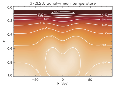
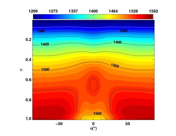
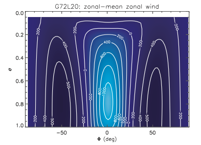
For each simulation we have followed Held & Suarez (1994) and Heng et al. (2011) and run the simulations for 1200 days (here, and throughout this work, ‘days’ refers to Earth days). The first 200 days are then discarded to allow for initial transients and ‘spin–up’, which is sufficient to span several relaxation times for the entire atmosphere in the SHJ case and for the upper atmosphere down to a pressure of $\sim 10^{5}$ Pa (or a few bar) for HD 209458b (using the radiative timescale of Iro et al., 2005). For the HD 209458b test case 1200 days is only sufficient to span $\sim 1$ radiative relaxation time throughout the radiative zone. Additionally, as the HD 209458b test case also includes a radiatively inactive region a significantly longer time is required to reach a statistical steady state (for example Cooper & Showman, 2005, found after 5000 days the atmosphere had reached a steady state down to $3\times 10^{5}$ Pa or $\sim$3 bar). The issue of whether the simulation has reached a statistically steady state will be discussed in more detail in Section 4.2. The solution from 200 to 1200 days is then used to create zonally and temporally averaged temperature and zonal wind plots, which we term ‘zonal mean’ plots (in a similar vein to Heng et al., 2011).

As discussed in section 2.5, to aid comparison with previous works we present plots using $\sigma$ (SHJ) and $\log(p)$ (HD 209458b) as our vertical coordinate, which we have created by interpolating the values from the geometric grids onto the isobaric surface required. The plots (throughout this work, for example Figure 1) feature contour lines (solid for positive and dashed for negative) that have been chosen, where applicable, to match those in Heng et al. (2011). These are complemented by colour scales, where a greater number of divisions (than the line contours) are used to aid qualitative interpretation of the data. The colour scales chosen have mostly been selected to match standard colour schemes in meteorology (i.e. blue–red for temperature). For wind plots we have adopted a blue–white–red colour scale where blue is retrograde or downdraft, i.e. negative wind, red is prograde or updraft, i.e. positive wind and white is positioned at zero.

3.1 Shallow–Hot Jupiter

3.1.1 Test case setup

The SHJ test is that prescribed by Menou & Rauscher (2009), a thin layer of a hypothetical tidally locked Jovian planet down to a depth of $1\times 10^{5}$ Pa or 1 bar. The equilibrium temperature profile is,

$$T_{\rm eq}=T_{\rm vert}+\beta_{\rm trop}\Delta T_{\rm EP}\cos(\lambda-180^{\circ})\cos(\phi),\\$$ (24)

where $T_{\rm vert}$ is given by,

$$T_{\rm vert}=\begin{cases}T_{\rm surf}-\Gamma_{\rm trop}(z_{\rm stra}+\frac{z-z_{\rm stra}}{2})\\ +\left(\left[\frac{\Gamma_{\rm trop}(z-z_{\rm stra})}{2}\right]^{2}+\Delta T_{\rm strat}^{2}\right)^{\frac{1}{2}}\mbox{,}\,&z\leq z_{\rm stra}\mbox{,}\\ T_{\rm surf}-\Gamma_{\rm trop}z_{\rm stra}+\Delta T_{\rm strat}\mbox{,}\,&z>z_{\rm stra}\mbox{.}\end{cases}$$

and $\beta_{\rm trop}$ is defined as

$$\beta_{\rm trop} =\begin{cases}\sin\frac{\pi(\sigma-\sigma_{\rm stra})}{2(1-\sigma_{\rm stra})}\mbox{,}\,&z\leq z_{\rm stra}\,\mbox{ or }\,\sigma\geq\sigma_{\rm stra}\mbox{,}\\ 0\mbox{,}\,&z>z_{\rm stra}\,\mbox{ or }\,\sigma<\sigma_{\rm stra}\mbox{.}\end{cases}$$

The values for the parameters featured in these equations are presented in Table 3. The radiative relaxation timescale throughout the entire atmosphere is set to $\tau_{\rm rad}=\pi/\Omega_{\rm p}\sim 1.731$ days.

We have run this test case using the “Full”, “Deep” and “Shallow” equation sets (see Table 1 for explanation), with the rest of the setup the same for each simulation. The number of vertical levels is 32 and the level top is placed at $3.29698\times 10^{6}$ m, no sponge layer was necessary and the diffusion has been applied to $u$, $v$ and $\theta$.

We started the atmosphere initially at rest and in vertical hydrostatic equilibrium using an isothermal temperature profile set at $1800$ K as used by Heng et al. (2011).

3.1.2 Results

The resulting flow and temperature of the “Shallow” SHJ test case at the $\sigma=0.675$ surface after 346 days, as well as the zonal mean plots are shown alongside the figures from Heng et al. (2011) (using their finite–grid model) in Figure 1. We present the instantaneous temperature field at $\sigma=0.675$ instead of the quoted value of 0.7 in Heng et al. (2011) as this quoted value does not represent the actual value of the surface, but the half–level just above it (i.e. at lower sigma and greater height). Therefore, the real $\sigma$ value is half the vertical resolution below the quoted $\sigma$ value (see Mayne et al., 2013, for a full discussion of this in regards to Earth–like tests).

Figure 1 shows that, qualitatively, we match the broad characteristics of the flow. Figure 2 then shows the same plots but for the “Full” case (the “Deep” case is omitted as it is virtually identical to the “Full”). Figure 2 shows an atmospheric structure broadly consistent with both the “Shallow” case and that of Heng et al. (2011). As the atmosphere of the SHJ is only $1\times 10^{5}$ Pa or 1 bar in extent its height is $\sim 4\times 10^{6}$m, and as the planetary radius is $R_{\rm p}=10^{8}$ (see Table 3), it is unsurprising that no difference is found when relaxing the ‘shallow–atmosphere’ approximation (see Table 1). Indeed the resulting flow is very similar in all cases. Some slight differences are present which will be discussed briefly in Section 4.1, but for now we move on to a more physically interesting test case.

Figure 1: Figure showing the solutions to the SHJ test case. Left panels are figures reproduced from Heng et al. (2011) using the finite–difference model (reproduced by permission of Oxford University Press), and the right panels are results from this work for the “Shallow” case (see Table 1 for explanation). The top row shows the temperature field at $\sigma=0.675$ and 346 days. The middle and bottom rows show the zonal mean plots for temperature and wind respectively (i.e. zonally and temporally, from 200-1200 days, averaged).

Figure 2: Figure matching those described in Figure 1 but for the “Full” case (see Table 1 for explanation).

3.2 HD 209458b

3.2.1 Test case setup

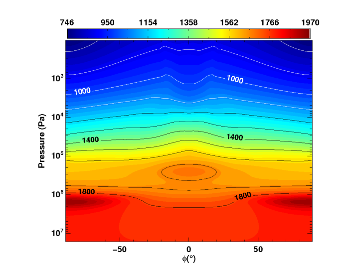
The test case for HD 209458b is a slightly adjusted version of that prescribed in Heng et al. (2011) (similar to that described in Rauscher & Menou, 2010), where the temperature and relaxation profiles are taken from the radiative equilibrium models of Iro et al. (2005). The domain encompasses a radiatively inactive region from $2.2\times 10^{7}$ to $1\times 10^{6}$ Pa (or 220 to 10 bar) (where $\tau_{\rm rad}=\infty$, termed ‘inactive’ in Heng et al., 2011) with a radiative zone above this.

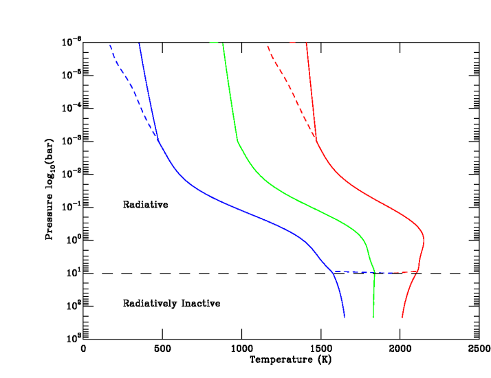
As discussed in Section 2.5 due to the horizontal gradients in pressure in the upper atmosphere, as we are using a height based approach and matching a test case performed in pressure coordinates we are including, necessarily, an extra section of computational domain i.e. the low pressure night side region. We found for our non–hydrostatic code the model was extremely unstable on the night side in this very cool low pressure region, leading to exponential growth of vertical velocities under small perturbations. Additionally, we found that the discontinuities in temperature across the $1\times 10^{6}$ Pa (or 10 bar) boundary found in the profile described in Heng et al. (2011) also led to instability (as discussed in Rauscher & Menou, 2010). Therefore, we have slightly adjusted the profiles of Heng et al. (2011). The most significant change, a modest heating of around 150 K, is performed in the region above $10^{-3}$ bar. This region is not included in the model of Heng et al. (2011), as their upper boundary is placed at this pressure. The altered temperature profiles are shown in Equations 27 and 28 and plotted in Figure 3 (with the radiative and radiatively inactive regions also indicated).

$$T_{\rm night}=\begin{cases}T_{\rm night}^{\prime}\rvert^{p_{\rm high}}+100{\rm K}\left(1.0-e^{-(\log(p)-\log(p_{\rm high}))}\right)\mbox{,}\,&p\geq p_{\rm high}\\ {\rm MAX}\left(T_{\rm night}^{\prime}\rvert^{p_{\rm low}}\times e^{0.10(\log(p)-\log(p_{\rm low}))},250\right)\mbox{,}\,&p<p_{\rm low}\\ T_{\rm night}^{\prime}\rvert^{p}\,&\mbox{otherwise}\end{cases}$$ (27)

$$T_{\rm day}=\begin{cases}T_{\rm day}^{\prime}\rvert^{p_{\rm high}}-120.0{\rm K}\left(1.0-e^{-(\log(p)-\log(p_{\rm high}))}\right)\mbox{,}\,&p\geq p_{\rm high}\\ {\rm MAX}\left(T_{\rm day}^{\prime}\rvert^{p_{\rm low}}\times e^{0.015(\log(p)-\log(p_{\rm low}))},1000\right)\mbox{,}\,&p<p_{\rm low}\\ T_{\rm day}^{\prime}\rvert^{p}\,&\mbox{otherwise}\end{cases}$$ (28)

$T_{\rm day}$ and $T_{\rm night}$ are the day and night side temperature profiles and $p$ is the pressure. $T_{\rm night}^{\prime}$ and $T_{\rm day}^{\prime}$ are the polynomial fits of Heng et al. (2011) to the day and night side profiles of Iro et al. (2005), and $p_{\rm low}$ and $p_{\rm high}$ are $100$ and $1\times 10^{6}$ Pa respectively (or $1\times 10^{-3}$ and $10$ bar).

Figure 3: Temperature–pressure profiles used for HD 209458b. The solid lines are from this work, and the dashed lines are the polynomial fits of Heng et al. (2011) to the models of Iro et al. (2005). The blue lines are the night side profiles, the red lines the day side profiles (i.e. $T_{\rm night}$ and $T_{\rm day}$, respectively) and the green line is the initial profile. The horizontal dashed line demarks the radiatively inactive and radiative regions.

The resulting profiles in Equations 27 and 28 are then combined to create a temperature map of the planet’s atmosphere using,

$$T_{\rm eq}=\\ \begin{cases}\left[T_{\rm night}^{4}+(T_{\rm day}^{4}-T_{\rm night}^{4})\cos(\lambda-180^{\circ})\cos\phi\right]^{\frac{1}{4}}\mbox{,}\,&90^{\circ}\leq\lambda\leq 270^{\circ}\\ T_{\rm night}\mbox{,}\,&\mbox{otherwise.}\\ \end{cases}$$ (29)

We have run this test case using the “Full”, “Deep” and “Shallow” equations sets with the top boundary placed at $1.1\times 10^{7}$ m and use 66 vertical levels (distributed uniformly in height). For this test case we require a sponge layer and minimise this for each simulation, where $\eta_{\rm s}=0.75$ in all cases. $C$ is 0.20 for both the “Deep” and “Shallow” case but 0.15 for the “Full” case. The effect of both the sponge layer and the use of uniform vertical levels (as opposed to those sampling, for instance, uniform $\log(p)$) have been explored and are briefly discussed in 4.2.

Each of the simulations has been initialised in hydrostatic equilibrium using a temperature profile midway between the day and night profiles (i.e. $(T_{\rm day}+T_{\rm night})/2$) and zero initial winds. As we are trying reproduce the results of a test case, we postpone a detailed exploration of the effect of varying initial conditions for later work (Mayne et al, in preparation).

3.2.2 Results

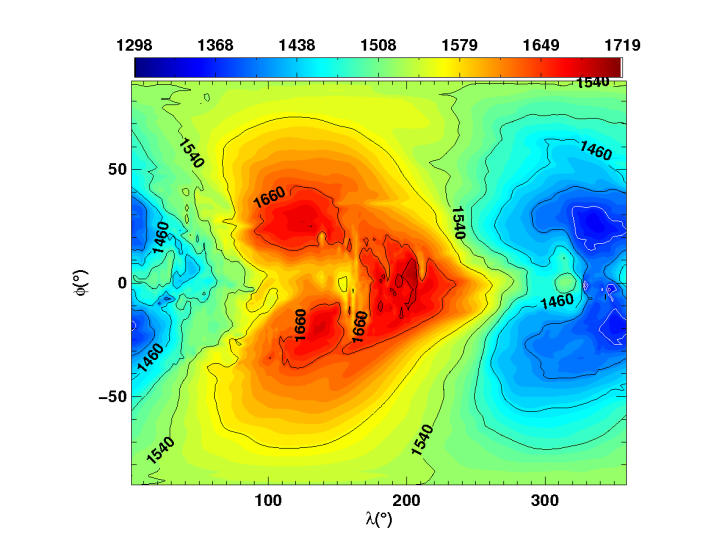
In general our resulting large–scale, long–term flows and those of Heng et al. (2011) for HD 209458b are qualitatively very similar.

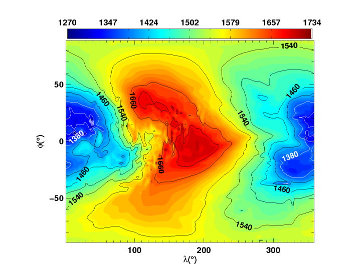
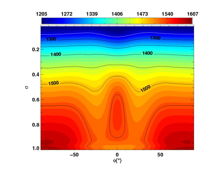
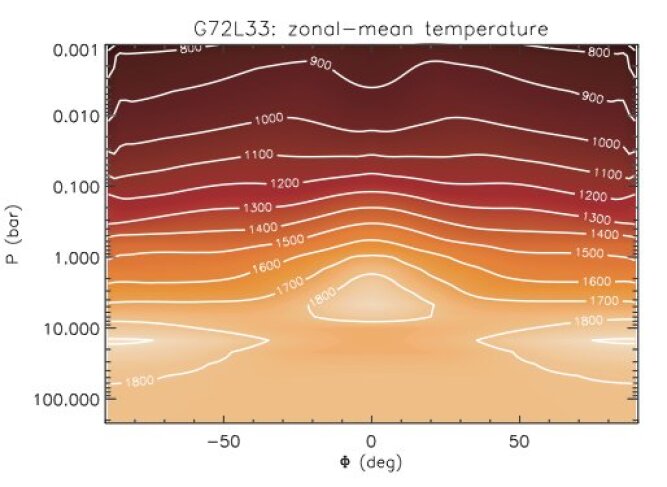
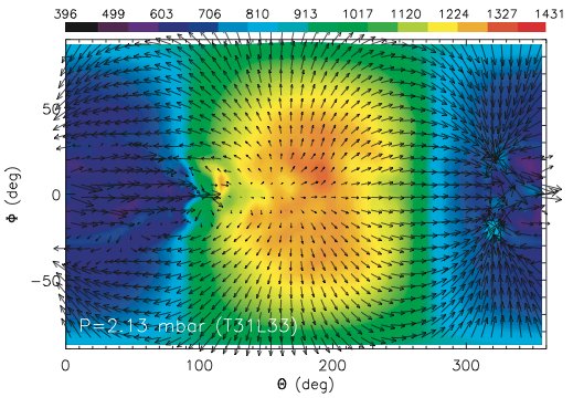
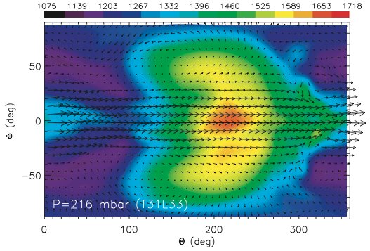
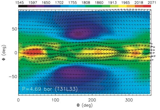
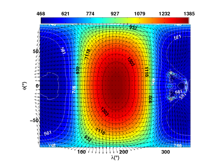
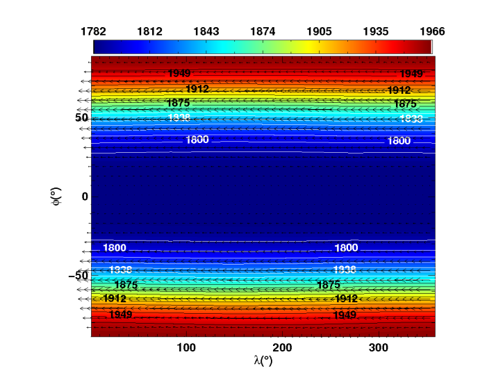
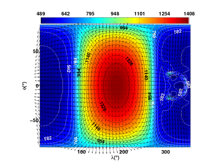
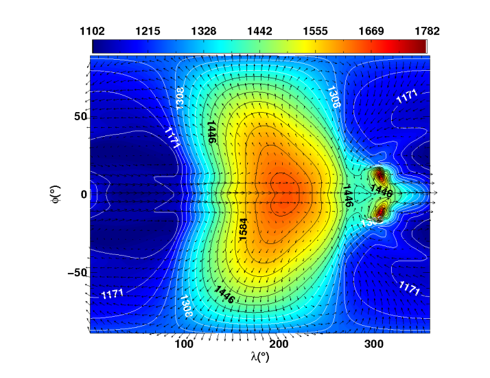
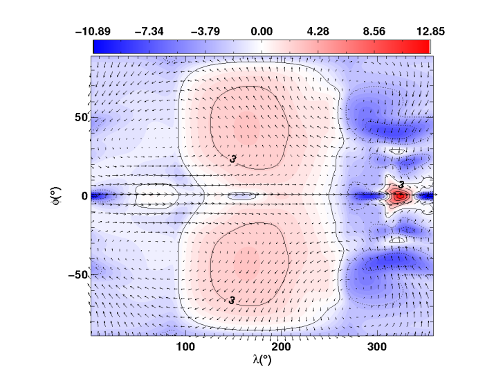
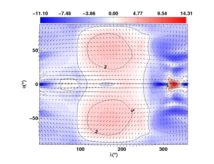
In order to aid comparison Figure 4 reproduces the results of Heng et al. (2011). Figure 4 shows snapshots of temperature and horizontal velocity for the same pressure levels (i.e. 213, 21 6000, 4.69$\times 10^{5}$ and 21.9$\times 10^{5}$ Pa) as in Heng et al. (2011) at 1200 days as found using their spectral code. Figure 4 also shows the zonal mean plots for the finite difference model of Heng et al. (2011). The same plots for our “Shallow” case are presented in Figure 5. We note that Heng et al. (2011) uses the pressure unit of bar, whereas we use SI units, Pa (where $1$ bar is $1\times 10^{5}$ Pa).

Figure 4: Figure showing results for the HD 209458b test case reproduced from Heng et al. (2011) (reproduced by permission of Oxford University Press). The top row shows the zonal mean plots (i.e. zonally and temporally, from 200-1200 days, averaged, using bar as the unit of pressure) of temperature (left) and zonal wind (right). The middle and bottom rows show the temperature (colour) and horizontal velocities (vectors) at pressures 213 (middle left), 21 600 (middle right), 4.69$\times 10^{5}$ (bottom left) and 21.9$\times 10^{5}$ Pa (bottom right) after 1200 days.

Figure 5: Figure matching those described in Figure 4 but for our “Shallow” case. The zonal mean plots present pressure in Pa (SI unit, where $1$ bar=$1\times 10^{5}$ Pa).

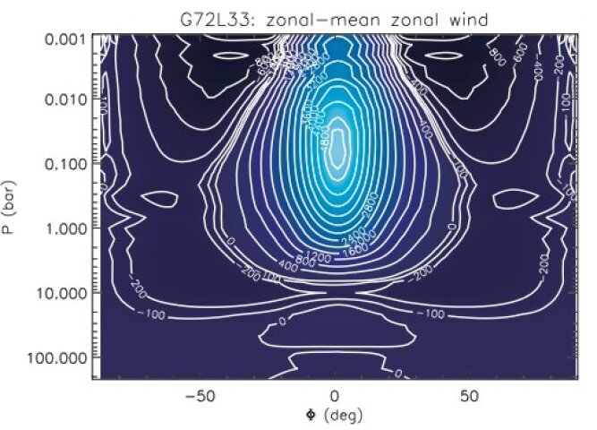
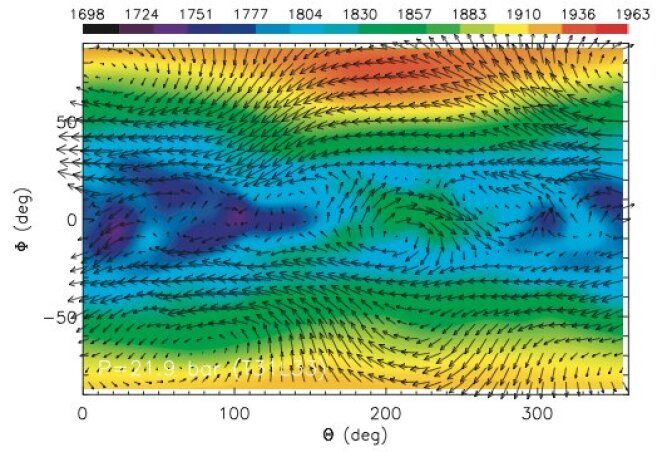
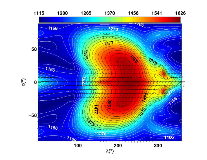
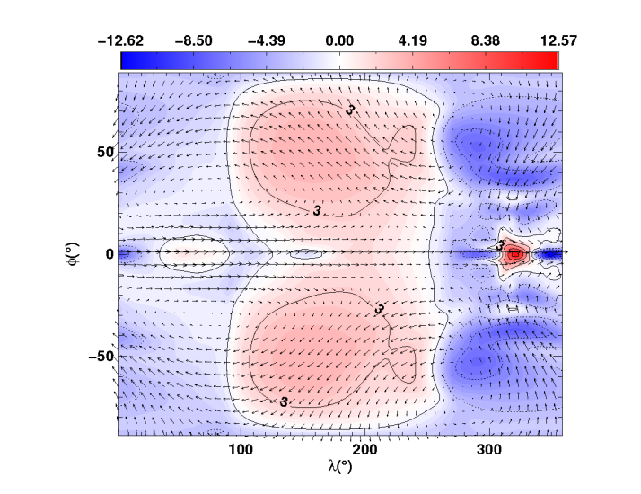
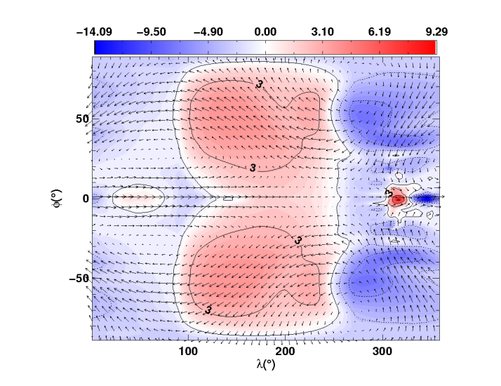
Figures 6 and 7 show the same plots as Figures 4 and 5 but for the “Deep” and “Full” cases, respectively. Comparing the results of Heng et al. (2011) reproduced in Figure 4 with our own results shown in Figures 5, 6 and 7, shows good, qualitative, agreement. In all cases we produce a wide, in latitude, prograde equatorial jet extending throughout the upper atmosphere from about $5\times 10^{5}$ Pa ($5$ bar) to $100$ Pa (or 1 mbar), flanked by retrograde winds. The temperature distribution also matches across the radiative zone. The jet does sharpen slightly, in latitude, and move to higher altitudes and lower pressures, as well as reducing in magnitude, when moving to the more sophisticated equation sets (i.e. “Shallow” to “Full”).

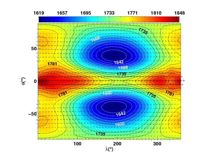
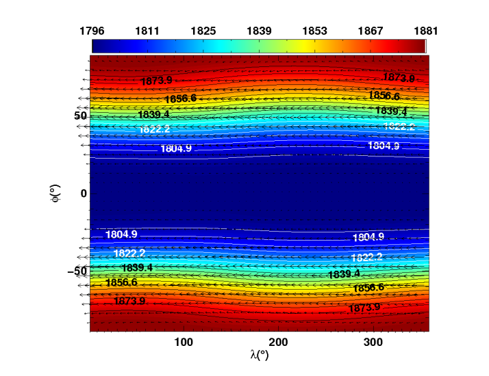
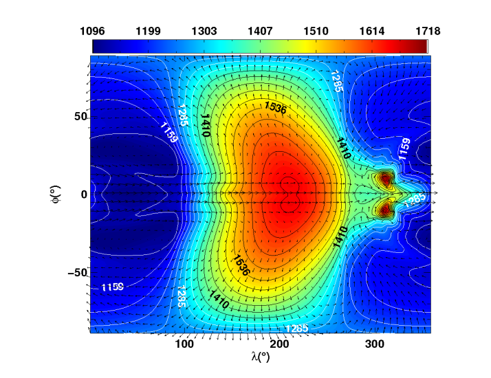
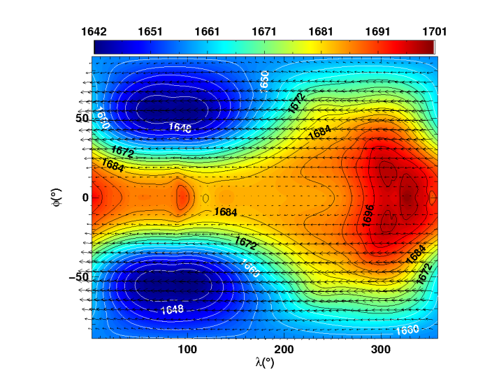
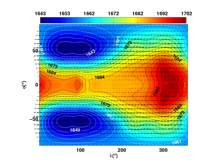
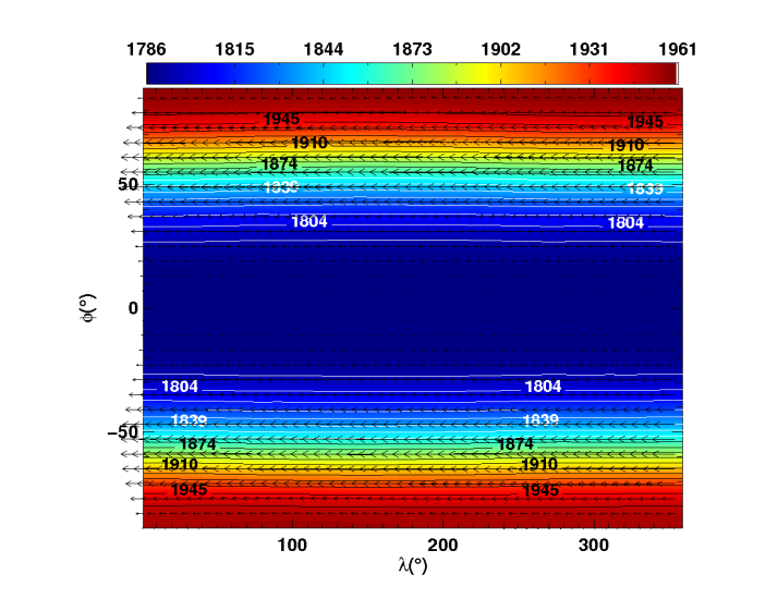
The instantaneous slices through the atmosphere at 213 and 21 600 Pa are also consistent across the figures presented. The 213 and 21 600 Pa isobaric surfaces exhibit diverging flow at the lower pressures and the development of a circumplanetary jet, with an associated shift in the temperature distribution at the higher pressure of the two surfaces. The temperature distributions also show little variation ($\Delta T\lesssim 150$K) across all simulations, which is unsurprising given the short radiative timescale at these pressures. At the higher pressure of 21.9$\times 10^{5}$ Pa the flow, morphologically, is still very similar, however the flow of Heng et al. (2011) appears less coherent. Additionally, slightly larger differences in temperature (than those found at the lower pressures) across the simulations appear, for the deepest isobaric surface. The pole, at depths, in the radiatively inactive region appears to become warmer as we move to the more complete (i.e. “Deep” and “Full”) dynamical equations.

The isobaric slice which shows the most difference between simulations is at 4.69$\times 10^{5}$ Pa. Here the flow morphology of the instantaneous field at 1200 days is quite different across the simulations, as is the associated temperature structure. Both the “Deep” and “Full” cases show a counter rotating, or westward moving flow at all latitudes. There is also a shift in the temperature distribution, with the regions of lowest temperature shifted to lower longitudes (i.e. westward). Despite the differences in the instantaneous slices at 4.69$\times 10^{5}$ Pa, the overall flow morphology is qualitatively very similar through each of simulations. Moreover, the time averaged flow and temperature structure, for all simulations, shows very little difference, despite the differences in numerical scheme, initial conditions and the equations solved.

Figure 6: Figure matching those described in Figure 4 but for our “Deep” case. The zonal mean plots present pressure in Pa (SI unit, where $1$ bar=$1\times 10^{5}$ Pa).

Figure 7: Figure matching those described in Figure 4 but for our “Full” case. The zonal mean plots present pressure in Pa (SI unit, where $1$ bar=$1\times 10^{5}$ Pa).

In Figure 8 we present the results from a subset of the simulations we have run demonstrating the relative invariance of the derived flow structure for this test case, over 1200 days. Here we term the standard simulations as those presented in Figures 5, 6 and 7. We have then run a set of simulations where we have changed individual parameters or settings to explore their effect, using each of the “Shallow” and “Full” equation sets. Here we present only a subset in order to sample the whole ‘parameter space’ with as few figures as possible.

As discussed in Section 2.6 we apply diffusion to the $u$ and $v$ fields only for this test case, in order to simply reproduce a more consistent result with that of Heng et al. (2011). The top left panel for Figure 8 shows the results for a simulations with exactly the same setup as the “Shallow” case shown in the top right panel of Figure 5, but with diffusion additionally applied to the $\theta$ field. The jet structure still persists but has shifted to higher pressures, sharpened in latitude and diminished, slightly diverging from the results of Heng et al. (2011) (as discussed in Section 2.6). This change is likely due to the effect of diffusion of the potential temperature on the baroclinically unstable regions flanking the equatorial jet. The details and changes in the underlying mechanism which ‘pumps’ the jet will be explored in a future publication (Mayne et al, in preparation). Despite the differences, the flanking retrograde jets are still present and the relative prograde to retrograde motions are similar to the previous simulations.

As mentioned in Section 2.5 we also adopt uniformly distributed (in geometric height) vertical levels for our standard HD 209458b simulations, as opposed to those uniform in $\log(p)$ (as adopted by Heng et al., 2011). The top right panel of Figure 8 shows the resulting flow for a simulations matching the “Full” case presented in the top right panel of Figure 7 but with only the vertical level distribution altered. The non-uniform level distribution used has been chosen to sample the local minimum atmospheric scaleheight. At each height, starting at the inner boundary, the smallest scaleheight (usually on the cooler night side) was found and three levels were placed within this scaleheight. The process was repeated till the height domain of the atmosphere ($1.1\times 10^{7}$ m) was reached (and resulted in a total of 78 vertical levels, compared to 66 for the standard simulations). Again, a similar flow morphology is found with a prograde jet flanked by retrograde jets, with only a modest sharpening of the jet apparent when compared to the standard “Full” case.

Finally, we have also, as detailed in Section 2.4 included a sponge layer in our upper boundary condition. Therefore, to explore the effect of this damping we have run two further simulations. The bottom right panel of Figure 8 shows a simulations where only the upper boundary has been altered from the standard “Full” case presented in Figure 7, and is placed at $1.25\times 10^{7}$ m above the inner boundary (using 80 vertical levels to retain a similar vertical resolution). As we increase the size of the domain, our upper boundary moves to lower pressures, however, in Figure 8 we only present the vertical section of the domain matching that encompassed by the standard “Full” case to aid comparison. For this simulation the damping layer only becomes non–negligible for pressure lower than $<100$ Pa, i.e. above the plotted region. As before, the flow does not diverge significantly from what one would expect of the simulations both of Heng et al. (2011) and others in this work.

Secondly, in the bottom left panel we present a simulation matching the standard “Shallow” case, presented in top right panel of Figure 5, except the upper boundary has been placed at $6.7\times 10^{6}$ m above the inner boundary (using 40 vertical levels, again to retain a similar vertical resolution), and does not include a damping layer in the upper boundary condition. Once more, the flow is approximately what one might expect from inspection of our standard case and those of Heng et al. (2011). The results presented in the bottom panels of Figure 8 indicate that the damping layer is not significantly altering our results besides its inclusion being physically preferable (by preventing reflection of gravity waves back into the domain at the upper boundary).

Figure 8 represents only a subset of the simulations we have run to explore the sensitivity to the parameters and numerical choices. However, all of the simulations not presented here show a similar qualitative flow structure, i.e. a prograde equatorial jet flanked by retrograde winds, over the 1200 day test period.

Figure 8: Figure showing the insensitivity of the zonally and temporally averaged zonal wind (ms^-1) to the different modelling choices. The simulations in the left panels use the “Shallow” and the right panels the “Full” equation set. The top left panel shows a simulations where diffusion is applied to $\theta$ in addition to $u$ and $v$. The top right panel shows a simulations with non–uniform vertical level placement to optimise sampling of the local scaleheight. The bottom left panel shows the results when the atmospheric height is decreased from $H=1.1\times 10^{7}$ m to $H=6.7\times 10^{6}$ m, and the bottom right panel when it is increased to $1.25\times 10^{7}$ m (although only the overlapping pressure domain of these simulations with that of the models in Heng et al. (2011), shown in Figure 4, is displayed to aid comparison).

The key conclusion one can draw from these results is that the general atmospheric structure is relatively invariant over 1200 days under a range of model choices. Therefore, the resulting zonal mean diagnostics plots for the HD 209458b test case (as presented in Heng et al., 2011) are qualitatively very similar for all models. When comparing our “Shallow” case with the primitive model of Heng et al. (2011) the agreement suggests that, for this test, the relaxation of the hydrostatic approximation and change in vertical coordinate (from $\sigma$ to height) is unimportant. Furthermore, although deviation is present in the snapshots and detail of the jet structures, further relaxation of the ‘shallow–fluid’ and ‘traditional’ approximations does not significantly alter the results (our “Deep” case). Finally, the additional relaxation of the constant gravity assumption (as represented by our “Full” case) also does not cause the long–term, large–scale atmospheric structure to change dramatically (i.e. the zonal mean plots). We have also shown that the results are relatively invariant to our numerical choices associated with diffusion, vertical resolution (and level placement) and the upper boundary sponge or damping layer. However, again slight differences in the detail of the flow structures are apparent.

4 Discussion

Despite the general concordance of our results with literature results, and across our different model types, some differences are apparent which we briefly discuss in this section. The zonal and temporal averaging involved in the zonal mean plots is intended to provide a robust way to compare the long–term and large–scale structure of the model atmospheres. Therefore, by design these plots are relatively insensitive to the more detailed differences in the atmospheres.

4.1 Shallow–Hot Jupiter

As discussed in Section 3 we have placed our vertical levels for the SHJ test case at positions emulating the $\sigma$ levels described in Heng et al. (2011). This process involved running a SHJ test case, with uniformly distributed vertical levels, to completion and zonally and temporally averaging the pressure structure to provide a mapping from height to pressure. During this process, the largest $\sigma$ value, i.e. the level closest to the inner boundary, leads to a very small (in vertical size) grid cell, which, even with a semi–implicit scheme, led to a numerical instability of the vertical velocity. Therefore, the lowest level was adjusted to create a larger (in vertical extent) bottom cell more numerically stable for a non–hydrostatic code.

Although our results for the SHJ are qualitatively similar to those of Heng et al. (2011) some differences are apparent. Most notably, perhaps, is the fact that our jets (prograde or retrograde) do not intersect either the boundary. No sponge layer is incorporated in the upper boundary for this test, but the result is unchanged when it is. This slight discrepancy between our results and those of Menou & Rauscher (2009) and Heng et al. (2011) is most likely caused by differences in domain or boundary conditions, as both boundaries intersect the flow features we are trying to capture. In this respect, i.e. likely dependency of the results on the domain and boundary conditions, the SHJ test is a poor benchmark.

4.2 HD 209458b

As explained in Sections 2.3.2 and 3, the prescribed test duration of 1200 days is only sufficient to span approximately one relaxation time for the deeper regions of the radiative zone. This, in addition to the fact it includes a radiatively inactive region which can only reach a relaxed or steady state through dynamical processes, suggests that 1200 days is insufficient for this case to reach a statistical steady state. Models based on the primitive equations have already shown that the deeper atmosphere will not reach a steady state in 1200 days. Both Cooper & Showman (2005) and Rauscher & Menou (2010) present evidence indicating that the atmosphere down to only $\sim 3\times 10^{5}$ Pa (or $\sim$3 bar) had relaxed in their models after 5000 and $\sim$600 days, respectively. Rauscher & Menou (2010) additionally, explicitly show that the kinetic energy is still evolving in the deeper regions of their modeled atmosphere after 1200 days. Additionally, models from the literature which include a more complete dynamical description, have been run for much shorter times than 1200 days. For example Dobbs-Dixon et al. (2010) run their simulations, which include the full dynamical equations, for only $\sim$ 100 days.

As suggested by Showman & Guillot (2002) a downward flux of kinetic energy was found in models of HD 209458b by Cooper & Showman (2005), therefore energy is transported into the deeper radiatively inactive region. Energy is also injected by the compressional heating. As discussed in Section 2.3.2 if one compares the equation sets used in our different models, as presented in Table 2, the terms affected as we move from a “Shallow” to a “Deep” and on to a “Full” equation set involve ‘exchange’ between the components of momentum, and importantly the vertical and horizontal components. Moreover, relaxing the constant gravity assumption, in particular, acts to weaken the stratification of the atmosphere. Therefore, it is plausible that as one moves to a more complete dynamical description, one allows the transfer of energy and momentum between the upper radiative atmosphere with short relaxation time (see discussion in Section 2.3), with both the deeper longer timescale radiative and the even deeper radiatively inactive regions.

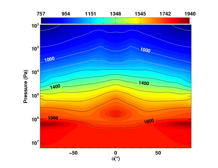
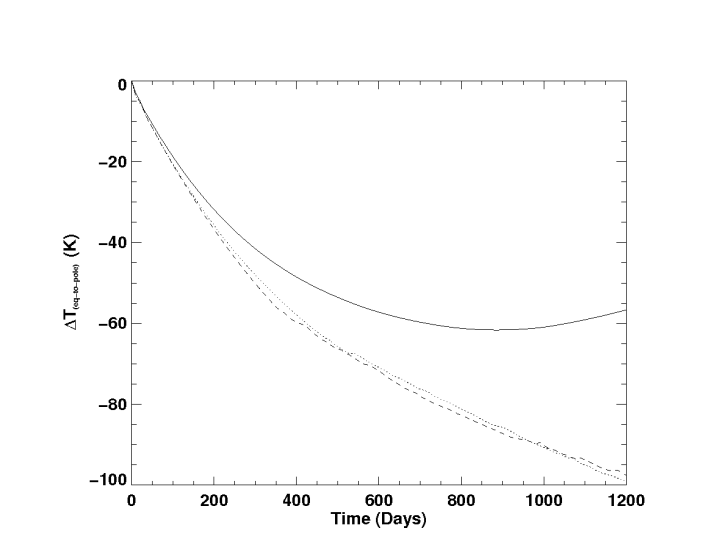
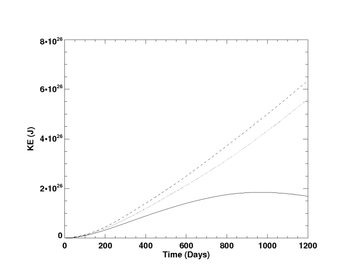
A retrograde flow in the deep region of the atmosphere must arise through an equatorward meridional flow (by conservation of angular momentum) or by vertical transport of angular momentum by waves or eddies, and must be accompanied by a warming of the polar regions relative to the equator (by thermal wind balance), which itself can only arise through a meridional circulation with descent near the poles and ascent near the equator. Figure 9 shows the vertically and zonally averaged equator–to–pole temperature difference (in the sense $T_{\rm equator}-T_{\rm pole}$), and total kinetic energy, for the radiatively inactive region (i.e. $p\geq 1\times 10^{6}$ Pa or 10 bar), for the HD 209458b test case and each equation set. Figure 9 shows evidence that the latitudinal temperature gradient in the deep atmosphere, and the kinetic energy, are approaching a steady state in the “Shallow” case. However, for both the “Deep” and “Full” cases the average latitudinal temperature gradient and total kinetic energy, are both still increasing by the end of the simulation. Additionally, Figure 9 shows that the average temperature difference between the equator and pole is larger in the “Deep” and “Full” cases than in the “Shallow” case, as is the total kinetic energy, in the radiatively inactive region. Figure 9, therefore, gives a strong indication both that the more simplified equation sets poorly represent the dynamical evolution of the deep atmosphere, and that the more sophisticated cases require a longer time to reach a statistically steady state.

The radiative timescale at the bottom of the radiative zone is $\tau_{\rm rad}\sim 500$ days, for HD 209458b. Therefore, given that below this the radiative timescale is infinite one would expect the timescale for relaxation of the radiatively inactive region to be $>>500$ days. The total elapsed time for the test cases performed in this work is 1200 days, suggesting it is unlikely the deep atmosphere will reach a relaxed state (an estimate supported by the data presented in Figure 9). Given that the angular momentum, and kinetic energy budget of the atmosphere can potentially be dominated by the deepest regions of the atmosphere, and the relaxation time of the deeper layers is long (compared to model elapsed times), it suggests that partially relaxed solutions to the entire atmospheric flow may not be persistent equilibrium states. It has been shown, for models solving the HPEs, that the results of such simulations are invariant to initial conditions (for discussion see Liu & Showman, 2012). However, as discussed in Section 2.3.2 the NHD equations include terms which act to exchange momentum between the vertical and horizontal motion. This exchange couples the shallow and deep atmosphere over long timescales meaning invariance to initial conditions cannot be proven until a statistical steady state throughout the model domain is reached. The alteration of the flow as the deeper layers become activated may lead to the establishment of a different equilibrium state (multiple equilibria are discussed in Liu & Showman, 2012), or it may move through a transient phase.

Problematically, for models such as the UM, and more specifically the ENDGame dynamical core, which solve the NHD equations, the interaction with the deeper layers is extremely slow and therefore exploration of this element may require huge computer resources (i.e. long integration times as mentioned in Showman et al., 2008). As a note of warning Viallet & Hameury (2008) demonstrate that for simulations of dwarf novae, where one side is strongly irradiated by the primary star, divergent flow is found, but no statistical steady state has been reached.

Figure 9: Figure showing the zonally and vertically averaged equator–to–pole temperature difference (top panel), and total kinetic energy (bottom panel) for the radiatively inactive region (i.e. $p\geq 1\times 10^{6}$ Pa or 10 bar), for the HD 209458b test case. The “Shallow”, “Deep” and “Full” cases are shown as the solid, dotted and dashed lines, respectively.

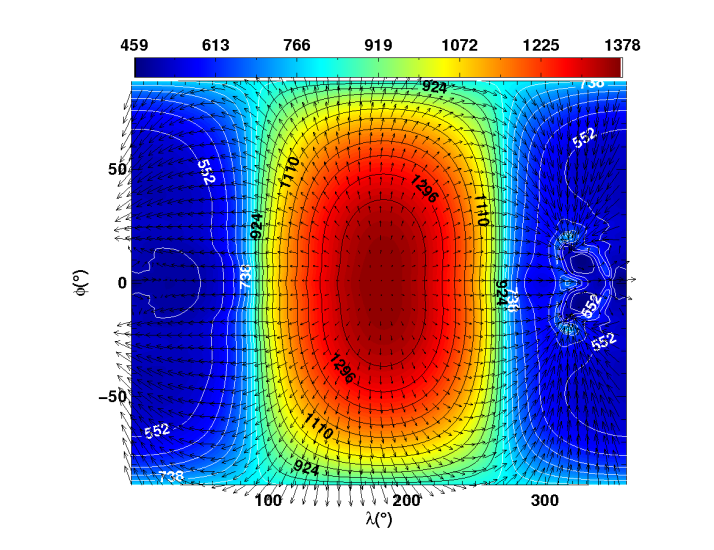
For our simulations, the zonal mean plots all show a prograde equatorial jet, demonstrating insensitivity of the mechanism which produces this feature to the dynamical equations used, over 1200 days. However, given that the radiatively inactive region, for the “Deep” and “Full” cases is clearly still evolving, one might expect the lower pressure regions of the atmosphere to also demonstrate evolution. The zonal mean plots show that the prograde equatorial jet is thinned (in latitude), contracted in height and diminished in magnitude, in the “Deep” and “Full” cases when compared to the “Shallow” case. Looking in detail at the time evolution of the flow one finds a largely invariant structure throughout most of the atmosphere in the “Shallow” case, where exchange between the vertical and horizontal momentum is inhibited. However, both the “Deep” and “Full” cases exhibit a varying large–scale flow structures. Figure 10 shows slices through the “Full” case at $1\times 10^{5}$ Pa (or 1 bar) at 100, 400, 800 and 1200 days (top left, top right, bottom left and bottom right panels, respectively).

The slices in Figure 10 show horizontal velocity (vectors) and the vertical velocity (colour scale). In this case (as is evident to a lesser degree in the “Deep” case) the large–scale flow is clearly still evolving. As the simulations runs the eastward jet, which is ‘spun–up’ in the first tens of days, gradually degrades and westward flow encroaches across the equator. This effect is seen, to differing degrees, throughout the atmosphere and leads to the thinning and diminishing of the jet when performing a zonal average. It is intriguing, that the departure of our results from the results of Heng et al. (2011) is most apparent when the constant gravity approximation is relaxed. This change acts to weaken the stratification and thereby increase the efficiency of vertical transport via, for instance, gravity waves.

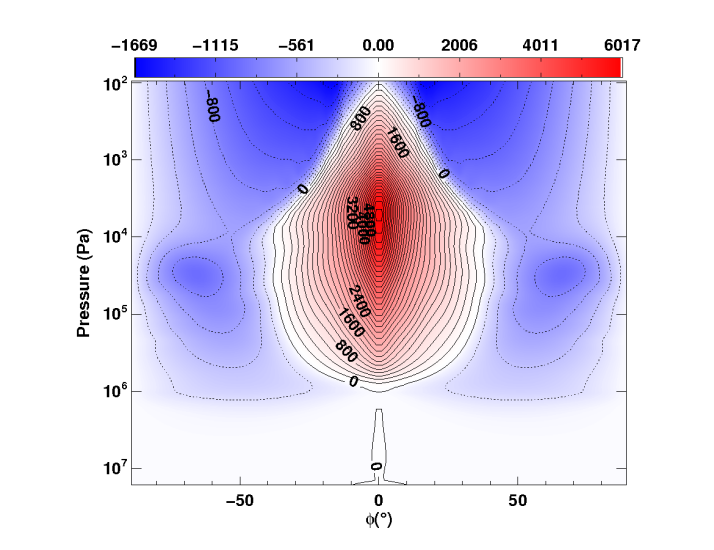
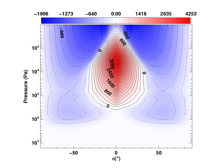
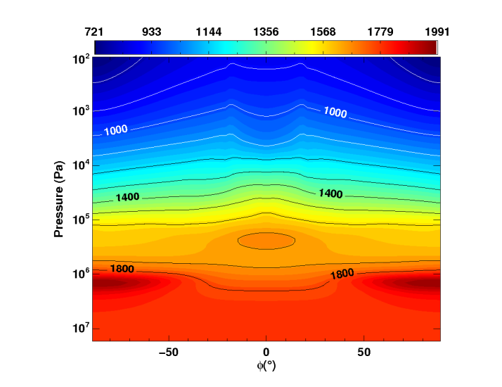
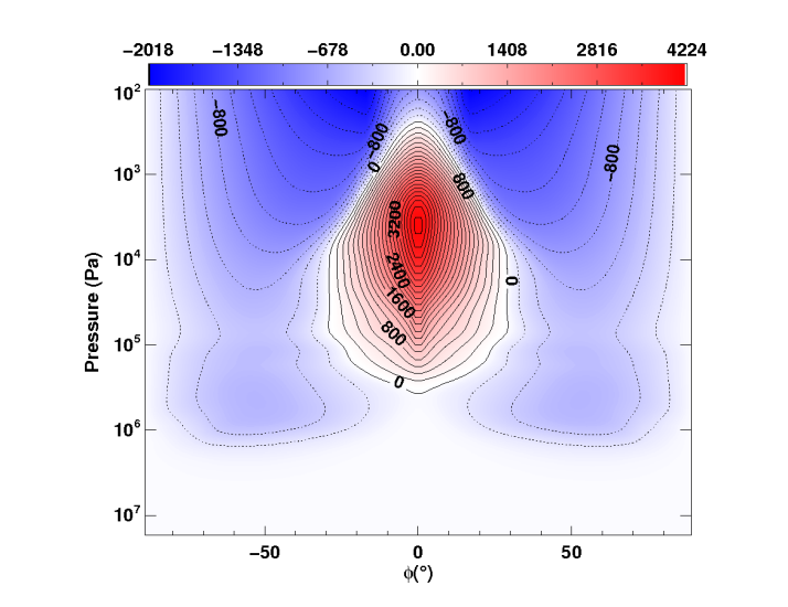
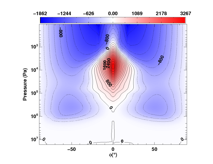
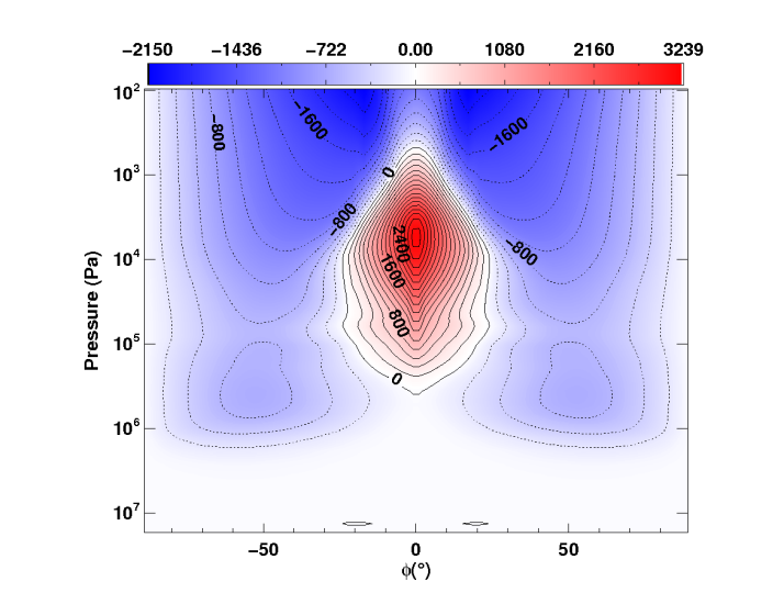
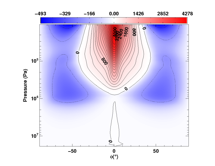
Figure 11 shows the time averaged (from 200 to 1200 days) vertical velocities for the “Shallow”, “Deep” and “Full” cases, as a function of pressure and either longitude (left panels) or latitude (right panels). In each case the field has been averaged in the horizontal dimension not plotted, i.e. if plotted as a function of latitude it has been zonally averaged. The meridional average is performed in a point–wise fashion, i.e. $\int\,vd\,\phi$ as opposed to $\int\,\cos\phi vd\,\phi$, to emphasise differences in vertical flow towards the polar regions. Figure 11 shows some significant differences in the vertical velocity profiles between the simulations. Firstly, the left panels show the meridionally averaged updraft is stronger, broader (in longitude) and larger in vertical extent in the “Full” case. However, the “Deep” case appears similar to the “Shallow”. Secondly, the right panels show, for the zonally averaged vertical circulation, as we move from the “Shallow” to “Deep” to “Full” cases, the updraft at the equator, and over the poles, strengthens, and the fast flowing downdrafts flanking the jet (in latitude), become stronger. Similar to jets on Earth, the regions flanking the jet are baroclinically unstable and will, therefore, generate eddies and perturbations, such as atmospheric Rossby waves. The interaction of these perturbations with the mean flow provides a mechanism to move energy (and angular momentum) up–gradient, i.e. into the jet, and therefore sustain the jets against dissipation.

Figure 10: Figure showing the horizontal velocity (vector arrows) and vertical velocity (colour scale) for the “Full” case (see Table 1 for explanation) at $1\times 10^{5}$ Pa (1 bar) and after 100 (top left), 400 (top right), 800 (bottom left) and 1200 (bottom right) days. Although the colour scales differ, the contour lines are the same for all panels.

Figure 11: Figure showing vertical velocity, as a function of pressure, for the “Shallow”, “Deep” and “Full” cases (see Table 1 for explanation) as the top, middle and bottom panels respectively. The left and right panels show vertical velocity as a function of longitude where a meridional average (performed in a point–wise fashion, i.e. $\int\,vd\,\phi$ as opposed to $\int\,\cos\phi vd\,\phi$, to emphasise differences in the vertical flow towards the polar regions) has been performed, and of latitude where a zonal average has been performed, respectively.

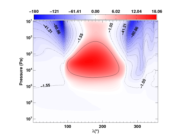
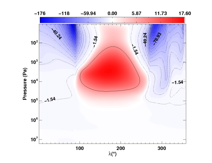
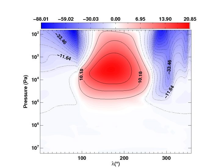
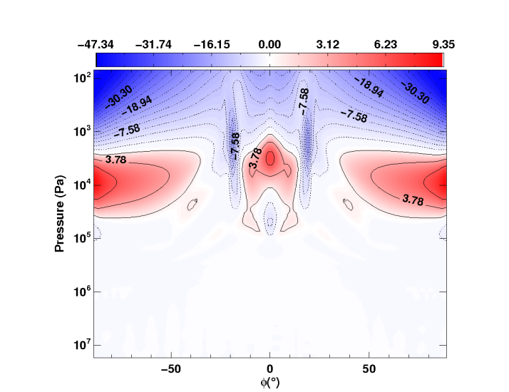
Showman & Polvani (2011) show that the jet pumping mechanism for hot Jupiters is unlikely to be similar to that relevant to Earth’s mid–latitude jets, i.e. the poleward motion of atmospheric Rossby waves. In fact the likely culprit, given the planetary scale of Rossby waves for hot Jupiters, is the interaction between standing atmospheric waves and the mean flow. Such standing waves are planetary in scale, and therefore are certainly poorly represented by any model which adopts the ‘traditional’ approximation (as discussed in White & Bromley, 1995). Additionally, Showman & Polvani (2011) show that the vertical transport of eddy momentum is a vital ingredient in the balance of superrotation at the equator. Therefore, it is clear that altering the efficiency of vertical transport will affect this mechanism, leading to a change in the balance of the pumping of the jet. Work is in progress to fully investigate this issue, which requires simulations run for a significantly longer integration time (Mayne et al, in preparation).

5 Conclusion

We have presented the first application of the UK Met Office global circulation model, the Unified Model, to hot Jupiters. In this work we have tested the ENDGame dynamical core (the component of a GCM which solves the equations of motion of the atmosphere) using a shallow–hot Jupiter (SHJ, as prescribed in Menou & Rauscher, 2009) and a HD 209458b test case (Heng et al., 2011). This work represents the first results of such test cases using a meteorological GCM solving the non–hydrostatic, deep–atmosphere equations. We have also completed the test case using the same code under varying levels of simplification to the governing dynamical equations. This work is complementary to the testing we have performed modelling Earth–like systems (Mayne et al., 2013).

In this work we suggest that, when relaxing the canonical simplifications made to the dynamical equations, the deeper regions of the radiative atmosphere, and the radiatively inactive regions, do not reach a steady state and are still evolving throughout the 1200 day test case. We have found that moving to a more complete description of the dynamics activates exchange between the vertical and horizontal momentum, and the deeper and shallower atmosphere. This leads to a degradation of the eastward prograde equatorial jet, and could represent either the beginnings of a new equilibrium state or multiple states, which may be dependent on the initial conditions of the radiatively inactive region of the atmosphere. In a future work we will investigate longer integration times, and explore the effect of simplifications to the dynamical equations on examples of jet pumping mechanisms in these objects. These results suggest that the test cases performed are not necessarily good benchmarks for a model solving the non–hydrostatic, deep–atmosphere equations.

We also aim to investigate the importance of the deeper atmosphere, and therefore, move the inner boundary for a HD 209458b simulation much deeper to $\sim 10^{8}$ Pa (or kbar) levels. This will require adaptation of the equation of state and increased flexibility in the prescription of $c_{p}$. These test cases have been performed using a Newtonian cooling scheme. As discussed in Showman et al. (2009) such a scheme does not include blackbody thermal emission of the gas itself, which can be significant when a region of heated material is advected into a region of net cooling. Using such a scheme the gas is just arbitrarily heated or cooled without taking into account its re-radiation into the surrounding area. In fact, as only the temperature is adjusted without knowledge of the specific heat capacity or quantity of material in a given cell (nor its optical properties) the energy deposited (or removed) from the system is unrepresentative. These problems can lead to regions where the heating or cooling is artificially high. To correct this we are adapting a non–grey radiative transfer scheme, under the two–stream approximation, which will be coupled to the UM dynamical core, ENDgame, under hot Jupiter conditions. The subsequent comparison to observations will be performed with a more physically meaningful model, once the coupling of our adapted schemes is complete.

The UM GCM is a powerful tool with which to study the effect, on the predicted states of exoplanet atmospheres, of both the interaction between the observable and deep atmosphere, and canonically made approximations to the governing dynamical equations. The ability to alter the level of simplification of the underlying dynamical equations (as provided by the ENDGame dynamical core) will prove vital as we explore exotic climate regimes where assumptions based on Earth’s atmosphere cannot a priori be assumed valid.