On the formation and physical properties of the Intra-Cluster Light in hierarchical galaxy formation models

Abstract

We study the formation of the Intra-Cluster Light (ICL) using a semi-analytic model of galaxy formation, coupled to merger trees extracted from N-body simulations of groups and clusters. We assume that the ICL forms by (1) stellar stripping of satellite galaxies and (2) relaxation processes that take place during galaxy mergers. The fraction of ICL in groups and clusters predicted by our models ranges between 10 and 40 per cent, with a large halo-to-halo scatter and no halo mass dependence. We note, however, that our predicted ICL fractions depend on the resolution: for a set of simulations with particle mass one order of magnitude larger than that adopted in the high resolution runs used in our study, we find that the predicted ICL fractions are  30-40 per cent larger than those found in the high resolution runs. On cluster scale, large part of the scatter is due to a range of dynamical histories, while on smaller scale it is driven by individual accretion events and stripping of very massive satellites, $M_{*}\gtrsim 10^{10.5}M_{\odot}$, that we find to be the major contributors to the ICL. The ICL in our models forms very late (below $z\sim 1$), and a fraction varying between 5 and 25 per cent of it has been accreted during the hierarchical growth of haloes. In agreement with recent observational measurements, we find the ICL to be made of stars covering a relatively large range of metallicity, with the bulk of them being sub-solar.

1 Introduction

The presence of a diffuse population of intergalactic stars in galaxy clusters was first proposed by Zwicky (1937), and later confirmed by the same author using observations of the Coma cluster with a 48-inch schmidt telescope (Zwicky 1952). More recent observational studies have confirmed that a substantial fraction of stars in clusters are not bound to galaxies. This diffuse component is generally referred to as Intra-Cluster Light (hereafter ICL).

Both from the observational and the theoretical point of view, it is not trivial to define the ICL component. A fraction of central cluster galaxies are characterized by a faint and extended stellar halo. These galaxies are classified as cD galaxies, where ‘c’ refers to the fact that these galaxies are very large and stands for supergiant and ‘D’ for diffuse (Matthews et al. 1964), to highlight the presence of a diffuse stellar envelope made of stars that are not bound to the galaxy itself. Separating these two components is not an easy task. On the observational side, some authors use an isophotal limit to cut off the light from satellite galaxies, while the distinction between the brightest cluster galaxy (hereafter BCG) and ICL is based on profile decomposition (e.g. Zibetti et al. 2005). Others (e.g. Gonzalez et al. 2005) rely on two-dimensional profile fittings to model the surface brightness profile of brightest cluster galaxies. In the framework of numerical simulations, additional information is available, and the ICL component has been defined using either a binding energy definition (i.e. all stars that are not bound to identified galaxies, e.g. Murante et al. 2007), or variations of this technique that take advantage of the dynamical information provided by the simulations (e.g. Dolag et al. 2010). In a recent work, Rudick et al. (2011) discuss different methods that have been employed both for observational and for theoretical data, and apply them to a suite of N-body simulations of galaxy clusters. They find that different methods can change the measured fraction of ICL by up to a factor of about four (from $\sim 9$ to $\sim 36$ per cent). In contrast, Puchwein et al. (2010) apply four different methods to identify the ICL in hydrodynamical SPH simulations of cluster galaxies, and consistently find a significant ICL stellar fraction ($\sim$ 45 per cent).

There is no general agreement in the literature about how the ICL fraction varies as a function of cluster mass. Zibetti et al. (2005) find that richer clusters (the richness being determined by the number of red-sequence galaxies), and those with a more luminous BCG have brighter ICL than their counterparts. However, they find roughly constant ICL fractions as a function of halo mass, within the uncertainties and sample variance. In contrast, Lin & Mohr (2004) empirically infer an increasing fraction of ICL with increasing cluster mass. To estimate the amount of ICL, they use the observed correlation between the cluster luminosity and mass and a simple merger tree model for cluster formation. Results are inconclusive also on the theoretical side, with claims of increasing ICL fractions for more massive haloes (e.g. Murante et al. 2004; Purcell et al. 2007; Murante et al. 2007; Purcell et al. 2008), as well as findings of no significant increase of the ICL fraction with cluster mass (e.g. Monaco et al. 2006; Henriques & Thomas 2010; Puchwein et al. 2010), at least for systems more massive than $10^{13}\,M_{\odot}/h$.

Different physical mechanisms may be at play in the formation of the ICL, and their relative importance can vary during the dynamical history of the cluster. Stars can be stripped away from satellite galaxies orbiting within the cluster, by tidal forces exerted either during interactions with other cluster galaxies, or by the cluster potential. This is supported by observations of arclets and similar tidal features that have been identified in the Coma, Centaurus and Hydra I clusters (Gregg & West 1998; Trentham & Mobasher 1998; Calcáneo-Roldán et al. 2000; Arnaboldi et al. 2012). As pointed out by several authors, in a scenario where galaxy stripping and disruption are the main mechanisms for the production of the ICL, the major contribution comes from galaxies falling onto the cluster along almost radial orbits, since tidal interactions by the cluster potential are strongest for these galaxies. Numerical simulations have also shown that large amounts of ICL can come from ‘pre-processing’ in galaxy groups that are later accreted onto massive clusters (Mihos 2004; Willman et al. 2004; Rudick et al. 2006; Sommer-Larsen 2006). In addition, Murante et al. (2007) found that the formation of the ICL is tightly linked to the build-up of the BCG and of the other massive cluster galaxies, a scenario supported by other theoretical studies (e.g. Diemand et al. 2005; Abadi et al. 2006; Font et al. 2006; Read et al. 2006). It is important, however, to consider that results from numerical simulations might be affected by numerical problems. Murante et al. (2007) find an increasing fraction of ICL when increasing the numerical resolution of their simulations. In addition, Puchwein et al. (2010) show that a significant fraction ($\sim 30$ per cent) of the ICL identified in their simulations forms in gas clouds that were stripped from the dark matter haloes of galaxies infalling onto the cluster. Fluid instabilities, that are not well treated within the SPH framework, might be able to disrupt these clouds suppressing this mode of ICL formation.

In this paper, we use the semi-analytic model presented in De Lucia & Blaizot (2007, hereafter DLB07), that we extend by including three different prescriptions for the formation of the ICL. We couple this model to a suite of high-resolution N-body simulations of galaxy clusters to study the formation and evolution of the ICL component, as well as its physical properties, and the influence of the updated prescriptions on model basic predictions (in particular, the galaxy stellar mass function, and the mass of the BCGs). There are some advantages in using semi-analytic models to describe the ICL formation with respect to hydrodynamical simulations: they do not suffer from numerical effects related to the fragility of poorly resolved galaxies, and allow the relative influence of different channels of ICL generation to be clearly quantified. However, the size and abundance of satellite galaxies (that influence the amount of predicted ICL) might be estimated incorrectly in these models. We will comment on these issues in the following.

The layout of the paper is as follows. In Section 2 we introduce the simulations used in our study, and in Section 3 we describe the prescriptions we develop to model the formation of the ICL component. In Section 4 we discuss how our prescriptions affect the predicted galaxy stellar mass function, and in Section 5 we discuss how the predicted fraction of ICL varies as a function of halo properties. In Section 6, we analyse when the bulk of the ICL is formed, and which galaxies provide the largest contribution. We then study the correlation between the ICL and the properties of the corresponding BCGs in Section 7, and analyse the metal content of the ICL in Section 8. Finally, we discuss our results and give our conclusions in Section 9.

2 N-body simulations

In this study we use collisionless simulations of galaxy clusters, generated using the ‘zoom’ technique (Tormen, Bouchet & White 1997, see also Katz & White 1993): a target cluster is selected from a cosmological simulation and all its particles, as well as those in its immediate surroundings, are traced back to their Lagrangian region and replaced with a larger number of lower mass particles. Outside this high-resolution region, particles of increasing mass are displaced on a spherical grid. All particles are then perturbed using the same fluctuation field used in the parent cosmological simulations, but now extended to smaller scales. The method allows the computational effort to be concentrated on the cluster of interest, while maintaining a faithful representation of the large scale density and velocity.

Below, we use 27 high-resolution numerical simulations of regions around galaxy clusters, carried out assuming the following cosmological parameters: $\Omega_{m}=0.24$ for the matter density parameter, $\Omega_{\rm bar}=0.04$ for the contribution of baryons, $H_{0}=72\,{\rm km\,s^{-1}Mpc^{-1}}$ for the present-day Hubble constant, $n_{s}=0.96$ for the primordial spectral index, and $\sigma_{8}=0.8$ for the normalization of the power spectrum. The latter is expressed as the r.m.s. fluctuation level at $z=0$, within a top-hat sphere of $8\,h^{-1}$Mpc radius. For all simulations the mass of each Dark Matter particle in the high resolution region of $10^{8}\,h^{-1}{\rm M}_{\odot}$, and a Plummer-equivalent softening length is fixed to $\epsilon=2.3h^{-1}$ kpc in physical units at $z<2$, and in comoving units at higher redshift.

Simulation data have been stored at 93 output times, between $z=60$ and $z=0$. Dark matter haloes have been identified using a standard friends-of-friends (FOF) algorithm, with a linking length of 0.16 in units of the mean inter-particle separation in the high-resolution region. The algorithm SUBFIND (Springel et al. 2001) has then been used to decompose each FOF group into a set of disjoint substructures, identified as locally overdense regions in the density field of the background halo. As in previous work, only substructures that retain at least 20 bound particles after a gravitational unbinding procedure are considered to be genuine substructures. Finally, merger histories have been constructed for all self-bound structures in our simulations, using the same post-processing algorithm that has been employed for the Millennium Simulation (Springel et al. 2005). For more details on the simulations, as well as on their post-processing, we refer the reader to Contini et al. (2012). For our analysis, we use a sample of 341 haloes extracted from the high resolution regions of these simulations, with mass larger than $10^{13}h^{-1}M_{\odot}$. In Table 1, we give the number of haloes in different mass ranges.

Table 1: The sample of haloes used in this study, split in five subsamples according to their mass. The first column indicates the mass range, and the second column gives the number of haloes in each subsample.

Halo mass range	Number of haloes
$\geq 10^{15}\,h^{-1}{\rm M}_{\odot}$	13
$[$5-10$]\times 10^{14}\,h^{-1}{\rm M}_{\odot}$	15
$[$1-5$]\times 10^{14}\,h^{-1}{\rm M}_{\odot}$	25
$[$5-10$]\times 10^{13}\,h^{-1}{\rm M}_{\odot}$	29
$[$1-5$]\times 10^{13}\,h^{-1}{\rm M}_{\odot}$	259

3 Semi-analytic models for the formation of the ICL

In this study, we use the semi-analytic model presented in DLB07, but we update it in order to include three different prescriptions for modelling the formation of the ICL component. These prescriptions are described in detail in the following. For readers who are not familiar with the terminology used within our model, we recall that we consider three different types of galaxies:

• Type 0: these are central galaxies, defined as those located at the centre of the main halo of each FOF group;

• Type 1: these are satellite galaxies associated with a distinct dark matter substructure. A Type 0 galaxy becomes Type 1 once its parent halo is accreted onto a more massive system;

• Type 2: also called orphan galaxies, these are satellites whose parent substructures have been stripped below the resolution limit of the simulation. Our reference model assumes that, when this happens, the baryonic component is unaffected and the corresponding galaxy survives for a residual time before merging with the corresponding central galaxy. The position of an orphan galaxy is traced by following the position of the particle that was the most bound particle of the parent substructure at the last time it was identified.

The residual merger time assigned to each galaxy that becomes Type 2 is estimated using the following implementation of the Chandrasekhar dynamical friction formula:

$$\tau_{merge}=f_{fudge}\frac{1.17}{\ln\Lambda}\frac{D^{2}}{R^{2}_{vir}}\frac{M_{par}}{M_{sat}}\tau_{dyn}$$ (1)

where $D$ is the distance between the satellite and the centre of its parent FOF, $R_{vir}$ is the virial radius of the parent halo, $M_{sat}$ the sum of the dark and baryonic mass of the satellite, $M_{par}$ the (dark matter) mass of the accreting halo, $\tau_{dyn}=R_{vir}/V_{vir}$ is the dynamical time of the parent halo, and $\Lambda=1+M_{par}/M_{sat}$ is the Coulomb logarithm. All quantities entering equation 1 are evaluated at the last time the substructure hosting the satellite galaxy is identified, before falling below the mass limit for substructure identification. As in DLB07, we have assumed $f_{fudge}=2$, which is in better agreement with recent numerical work indicating that the classical dynamical friction formulation tends to under-estimate the merging times measured from simulations (Boylan-Kolchin et al. 2008; Jiang et al. 2008).

The reference model does not include a prescription for the formation of the ICL. Below, we describe three different models that we have implemented to account for the ICL component. We assume that it is formed through two different channels: (i) stellar stripping from satellite galaxies and (ii) relaxation processes that take place during mergers and may unbind some fraction of the stellar component of the merging galaxies. In the following, we describe in detail each of our prescriptions.

3.1 Disruption Model

This model is equivalent to that proposed by Guo et al. (2011), and assumes that the stellar component of satellite galaxies is affected by tidal forces only after their parent substructures have been stripped below the resolution of the simulation (i.e. the galaxies are Type 2). We assume that each satellite galaxy orbits in a singular isothermal potential,

$$\phi(R)=V_{vir}^{2}\ln R,$$ (2)

and assume the conservation of energy and angular momentum along the orbit to estimate its pericentric distance:

$$\left(\frac{R}{R_{peri}}\right)^{2}=\frac{\ln R/R_{peri}+\frac{1}{2}(V/V_{vir})^{2}}{\frac{1}{2}(V_{t}/V_{vir})^{2}}.$$ (3)

In the equation above, $R$ is the distance of the satellite from the halo centre, and $V$ and $V_{t}$ are the velocity of the satellite with respect to the halo centre and its tangential part, respectively. Following Guo et al. (2011), we compare the main halo density at pericentre with the average baryon mass density (i.e. the sum of cold gas mass and stellar mass) of the satellite within its half mass radius. Then, if the following condition is verified:

$$\frac{M_{DM,halo}(R_{peri})}{R_{peri}^{3}}=\rho_{DM,halo}>\rho_{sat}=\frac{M_{sat}}{R_{half}^{3}}\,,$$ (4)

we assume the satellite galaxy to be disrupted and its stars to be assigned to the ICL component of the central galaxy. In the equation above, we approximate $R_{half}$ by the mass weighted average of the half mass radius of the disk and the half mass radius of the bulge, and $M_{sat}$ is the baryonic mass (cold gas plus stellar mass). The cold gas mass that is associated with the disrupted satellite is added to the hot component of the central galaxy. When a central Type 0 galaxy is accreted onto a larger system and becomes a Type 1 satellite, it carries its ICL component until its parent substructure is stripped below the resolution limit of the simulation. At this point, its ICL is added to that of the new central galaxy.

In a recent paper, Villalobos et al. (2012) discuss the limits of this implementation with respect to results from controlled numerical simulations of the evolution of disk galaxies within a group environment. The model discussed above is applied only after the galaxy’s dark matter subhalo has been completely disrupted, but the simulations by Villalobos et al. show that the stellar component of the satellite galaxy can be significantly affected by tidal forces when its parent subhalo is still present. In addition, this model assumes that the galaxy is completely destroyed when equation (4) is satisfied, but the simulations mentioned above show that galaxies can survive for a relatively long time (depending on their initial orbit) after they start feeling the tidal forces exerted by the cluster potential.

Predictions from this model are affected by numerical resolution. We carried out a convergence test by using a set of low-resolution simulations with the same initial conditions of the high-resolution set used in this paper, but with the dark matter particle mass one order of magnitude larger than the one adopted in the high resolution set and with gravitational softening increased accordingly by a factor $10^{1/3}$. We find that, on average, the ICL fraction is $\sim 30$ per cent higher in the low-resolution set ($\sim 20$ per cent in group-like haloes with mass $\sim 10^{13}M_{\odot}h^{-1}$ and $\sim 50$ in the most massive haloes considered in our study, as shown in the right panel of Figure 14 in Appendix A). This is due to the fact that, decreasing the resolution, a larger fraction of satellite galaxies are classified as Type 2 and are subject to our stripping model. While the lack of numerical convergence does not affect the qualitative conclusions of our analysis, we point out that the amount of ICL measured in our simulations should be regarded as an upper limit.

3.2 Tidal Radius Model

In this prescription, we allow each satellite galaxy to lose mass in a continuous fashion, before merging or being totally destroyed. Assuming that the stellar density distribution of each satellite can be approximated by a spherically symmetric isothermal profile, we can estimate the tidal radius by means of the equation:

$$R_{t}=\left(\frac{M_{sat}}{3\cdot M_{DM,halo}}\right)^{1/3}\cdot D$$ (5)

(Binney & Tremaine 2008). In the above equation, $M_{sat}$ is the satellite mass (stellar mass + cold gas mass), $M_{DM,halo}$ is the dark matter mass of the parent halo, and $D$ the satellite distance from the halo centre.

In our model, a galaxy is a two-component system with a spheroidal component (the bulge), and a disk component. If $R_{t}$ is smaller than the bulge radius, we assume the satellite to be completely disrupted and its stellar and cold mass to be added to the ICL and hot component of the central galaxy, respectively. If $R_{t}$ is larger than the bulge radius but smaller than the disk radius, we assume that the mass in the shell $R_{t}-R_{sat}$ is stripped and added to the ICL component of the central galaxy. A proportional fraction of the cold gas in the satellite galaxy is moved to the hot component of the central galaxy. We assume an exponential profile for the disk, and $R_{sat}=10\cdot R_{sl}$, where $R_{sl}$ is the disk scale length ($R_{sat}$ thus contains 99.9 per cent of the disk stellar mass). After a stripping episode, the disk scale length is updated to one tenth of the tidal radius.

This prescription is applied to both kinds of satellite galaxies. For Type 1 galaxies, we derive the tidal radius including the dark matter component in $M_{sat}$, and we impose that stellar stripping can take place only if the following condition is verified:

$$R^{DM}_{half}<R^{Disk}_{half}\,,$$ (6)

where $R^{DM}_{half}$ is the half-mass radius of the parent subhalo, and $R^{Disk}_{half}$ the half-mass radius of the galaxy’s disk, that is $1.68\cdot R_{sl}$ for an exponential profile. When a Type 1 satellite is affected by stellar stripping, the associated ICL component is added to that of the corresponding central galaxy.

As for the Disruption model, predictions from the Tidal Radius model are affected by numerical resolution. We carried out the same convergence test used for the Disruption model. Again, we find for the low resolution set a larger amount of ICL (by about 40 per cent, almost independent of halo mass, as shown in the left panel of Figure 14 in Appendix A). In this model, Type 2 galaxies are the dominant contributors to the ICL and, as for the Disruption model, the larger number of these satellites in the low-resolution set translates in a larger number of galaxies eligible for tidal stripping.

3.3 Continuous Stripping Model

This model is calibrated on recent numerical simulations by Villalobos et al. (2012). These authors have carried out a suite of numerical simulations aimed to study the evolution of a disk galaxy within the global tidal field of a group environment (halo mass of about $10^{13}\,{\rm M}_{\odot}$). In the simulations, both the disk galaxy and the group are modelled as multi-component systems composed of dark matter and stars. The evolution of the disk galaxy is followed after it crosses the group virial radius, with initial velocity components consistent with infalling substructure from cosmological simulations (see Benson 2005). The simulations cover a broad parameter space and allow the galaxy-group interaction to be studied as a function of orbital eccentricity, disk inclination, and galaxy-to-group mass ratio. We refer to the original paper for a more detailed description of the simulations set-up, and of the results.

Analysing the outputs of these simulations (Villalobos et al, in preparation), we have derived a fitting formula that describes the evolution of the stellar mass lost by a satellite galaxy as a function of quantities estimated at the time of accretion (i.e. at the time the galaxy crosses the virial radius of the group). Our fitting formula reads as follow:

$$M^{*}_{lost}=M^{*}_{accr}\exp\left[\left(\frac{-16}{1-\eta}\right)\left(\frac{M_{sub}}{M_{par}}\right)^{\frac{1}{2}}\left(1-\frac{t}{t_{merg}}\right)\right]$$ (7)

where $M^{*}_{accr}$ is the stellar mass at the time of accretion, $\eta$ is the circularity of the orbit, $M_{sub}$ and $M_{par}$ are the subhalo and parent halo dark matter masses respectively, and $t_{merg}$ is the residual merger time of the satellite galaxies. We approximate the accretion time as the last time the galaxy was a central galaxy (a Type 0), and compute the circularity using the following equation:

$$\eta=V_{\theta}\sqrt{\frac{2f-V^{2}_{r}-V^{2}_{\theta}}{2f-1}},$$ (8)

where $V_{r}$ and $V_{\theta}$ are the radial and tangential velocities of the accreted subhalo, and $f=1+M_{sub}/M_{par}$. For each accreted galaxy, $V_{r}$ and $V_{\theta}$ are extracted randomly from the distributions measured by Benson (2005) from numerical simulations.

Since Eq. 7 is estimated at the time of accretion, we cannot use the merger time prescription that is adopted in the reference model, where a residual merger time is assigned only at the time the substructure is stripped below the resolution of the simulation. To estimate merger times at the time of accretion, we use the fitting formula by Boylan-Kolchin et al. (2008) (hereafter BK08), that has been calibrated at the time the satellite galaxy crosses the virial radius of the accreting system, and is therefore consistent with our Eq. 7. In a few cases, it happens that the merger time is elapsed when the satellite galaxy is still a Type 1. In this case, we do not allow the galaxy to merge before it becomes a Type 2.

De Lucia et al. (2010) compared the merger times predicted using this formula with no orbital dependency and for circular orbits with those provided by Equation 1 used in the reference model, and found a relatively good agreement. We find that, once the orbital dependency is accounted for, the BK08 fitting formula predicts merger times that are on average shorter than those used in our reference model by a factor of $\sim 3$ for mass-ratios $M_{sub}/M_{par}>0.025$. Therefore, in our continuous stripping model, mergers are on average shorter than in the disruption and tidal radius models.

To implement the model described in this section for the formation of the ICL, we use Eq. 7 to compute how much stellar mass has to be removed from each satellite galaxy at each time-step. The stripped stars are then added to the ICL component of the corresponding central galaxy, and a proportional fraction of the cold gas in the satellite is moved into the hot component associated with the central galaxy. If the stripped satellite is a Type 1, and it carries an ICL component, this is removed at the first episode of stripping and added to the ICL component of the central galaxy.

It is worth stressing that Eq. 7 is valid for disk galaxies that are accreted on a system with velocity dispersion typical of a galaxy group, and that we are extrapolating the validity of this equation to a wider halo mass ranges.

3.4 Merger channel for the formation of the ICL

Murante et al. (2007) argue that the bulk of the ICL is not due to tidal stripping of satellite galaxies (that in their simulations accounts for no more than 5-10 per cent of the total diffuse stellar component), but to relaxation processes taking place during the mergers that characterize the build-up of the central dominant galaxy.

In our reference model, if two galaxies merge, the stellar mass of the merging satellite is added to the stellar (bulge) mass of the central galaxy. Based on the findings described above, we add a ‘merger channel’ to the formation of the ICL by simply assuming that, when two galaxies merge, 20 per cent of the satellite stellar mass gets unbound and is added to the ICL of the corresponding central galaxy. We have verified that this simple prescriptions reproduces approximately the results of the numerical simulations by Villalobos et al. (2012), though in reality the fraction of stars that is unbound should depend on the orbital circularity (Villalobos et al., in preparation). We have also verified that assuming that a larger fraction of the satellite stellar mass gets unbound, obviously leads to higher ICL fractions. In particular, assuming that 50 per cent of the stellar mass of the satellite is unbound, almost doubles the ICL fractions predicted. Assuming an even higher fraction does not affect further the ICL fraction because the effect of having more stellar mass unbound is balanced by the fact that merging galaxies get significantly less massive.

A similar prescription was adopted in Monaco et al. (2006) who showed that this has important consequences on the assembly history of the most massive galaxies, and in Somerville et al. (2008) as one possible channel for the formation of the ICL in the context of a hierarchical galaxy formation model. In order to test the influence of this channel on our results, in the following we will present results with this channel both on and off.

3.5 Modelling the bulge and disk sizes

Our reference model (DLB07) does not include prescriptions to model the bulge size, that we use in our stellar stripping models. To overcome this limitation, we have updated the reference model including the prescriptions for bulge and disk growth described in Guo et al. (2011).

Both the gaseous and stellar components of the disk are assumed to follow an exponential profile. Assuming a flat circular velocity curve, the scale-lengths of these two components can be written as:

$$R^{g}_{sl}=\frac{J_{gas}/M_{gas}}{2V_{max}},\hskip 28.45274ptR^{*}_{sl}=\frac{J_{*}/M_{*,disk}}{2V_{max}},$$ (9)

where $J_{gas}$ and $J_{*}$ are the angular momenta of the gas and stars, $M_{gas}$ and $M_{*,disk}$ are the gas and stellar mass of the disk, and $V_{max}$ is the maximum circular velocity of the dark halo associated with the galaxy. Following Guo et al. (2011), we assume that the change in the angular momentum of the gas disk during a timestep can be expressed as the sum of the angular momentum changes due to addition of gas by cooling, accretion from minor mergers, and gas removal through star formation. The latter causes a change in the angular momentum of the stellar disk. We refer to the original paper by Guo et al. for full details. We have verified that switching back to the simple model for disk sizes of Mo et al. (1998) used in our reference model, does not affect significantly the results discussed in the following.

Bulges grow through two different channels: mergers (both major and minor) and disk instability. Following Guo et al. (2011), we estimate the change in size due to a merger using energy conservation and the virial theorem:

$$\frac{GM_{new,b}^{2}}{R_{new,b}}=\frac{GM_{1}^{2}}{R_{1}}+\frac{GM_{2}^{2}}{R_{2}}+\frac{M_{1}M_{2}}{R_{1}+R_{2}}$$ (10)

The same approach is adopted in case of disk instability, simply replacing $R_{1}$ and $M_{1}$ with the size and mass of the existing bulge, and $R_{2}$ and $M_{2}$ with the size and mass of the stars that are transferred from the disk to the bulge so as to keep the disk marginally stable. $R_{2}$ is determined assuming that the mass is transferred from the inner part of the disk, with the newly formed bulge occupying this region. Again, we refer to the original paper by Guo et al. (2011) for full details on this implementation.

4 The Galaxy Stellar Mass Function

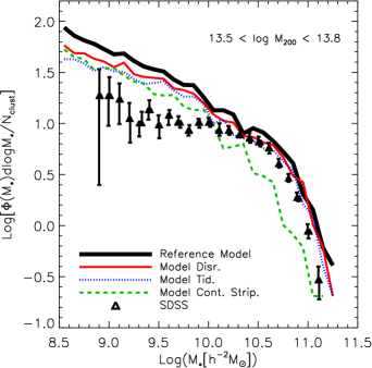
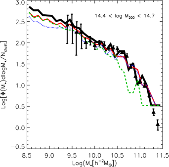
Figure 1: Left panel: The conditional stellar mass function of satellite galaxies in haloes in the mass range $13.5<\log M_{200}[M_{\odot}h^{-1}]<13.8$. Our simulations provide a total of 49 haloes in this mass range. Predictions from our reference model (DLB07) are shown by a solid black line, while predictions from our three models including disruption or/and stripping of satellite galaxies are shown by thinner lines of different style, as indicated by the legend. Symbols with error bars show observational measurements based on SDSS by Liu et al. (2010). Right panel: as in the left panel, but for the 3 haloes from our simulations with $14.4<\log M_{200}[M_{\odot}h^{-1}]<14.7$.

Before focusing our discussion on the ICL component, it is interesting to analyse how the proposed prescriptions affect one basic prediction of our model, that is the galaxy stellar mass function. In Figure 1, we show the conditional stellar mass function of satellite galaxies in the 49 haloes from our simulations that fall in the mass range $13.5<\log M_{200}[M_{\odot}h^{-1}]<13.8$ in the left panel, and in the 3 haloes from our simulations with $14.4<\log M_{200}[M_{\odot}h^{-1}]<14.7$ in the right panel. We show predictions from both our reference model (DLB07, shown as a solid black line), and from the three models including the treatments for the stripping and/or disruption of satellite galaxies discussed in Section 3 (lines of different style, see legend). Model predictions are compared with observational measurements by Liu et al. (2010). These are based on group catalogues constructed from the Sloan Digital Sky Survey (SDSS) Data Release 4, using all galaxies with extinction corrected magnitude brighter than $r=18$ and in the redshift range $0.01\leq z\leq 0.2$. We do not show here predictions from the models with the merger channel for the formation of the ICL switched on, as these do not deviate significantly from the corresponding models with the merger channel off.

For the lower halo mass range considered, the reference model fails in reproducing the observed stellar mass function, over-predicting the abundance of galaxies with stellar mass below $\sim 10^{10}\,{\rm M}_{\odot}$. This problem is somewhat alleviated when including a model for stellar stripping, but not solved. In particular, our ‘disruption model’ (model Disr. in the figure and hereafter) does not significantly affect the abundance of the most massive satellites, while reducing the number of their lower mass counterparts (not by the amount required to bring model predictions in agreement with observational results). This is expected as this model only acts on Type 2 galaxies, that dominate the low-mass end of the galaxy mass function.

Predictions from the ‘tidal radius model’ (model Tid.) are not significantly different from those of model Disr., while the ‘continuous stripping model’ (model Cont. Strip.) significantly under-predicts the abundance of the most massive satellite galaxies. There are two possible explanations for this behaviour: (i) the abundance of massive satellites is reduced because these are significantly affected by our stripping model or (ii) these massive satellites have disappeared because they have merged with the central galaxies of their parent haloes. As discussed in Section 3.3, our model Cont. Strip. uses a different prescription for merger times with respect to that employed in the reference model and in models Disr. and Tid. We find that, in this model, merger times are on average shorter than in the other models, which is the reason for the under-prediction of massive satellites shown in Figure 1. As we will discuss in the following, this also implies that the stellar mass of the BCGs in model Cont. Strip. are on average larger than those predicted by models Disr. and Tid.

For the higher halo mass range considered, the observed number density of intermediate-to-low mass galaxies is higher, and all our models appear to be in agreement with observational measurements. The agreement remains good also at the massive end, with the exception of model Cont. Strip. that significantly under-predicts the number density of massive galaxies. As explained above, this is due to the shorter galaxy merger times used in this model.

We will show below that, in our models, the merger channel does not provide the dominant contribution to the ICL formation so that this is mainly driven by stripping and/or disruption of satellites. Therefore, the excess of intermediate to low-mass galaxies for haloes in the lower mass range might invalidate our predictions. However, as we will show below, the bulk of the ICL originates from relatively massive galaxies so that this particular failure of our models does not significantly affect our results.

5 ICL fraction and dependency on halo properties

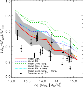
Figure 2: Left panel: ICL fraction as a function of halo mass. Lines of different style and colour show median results from different models, as indicated in the legend. Right panel: ratio between the ICL component plus BCG stellar mass and the total stellar mass within $R_{500}$. Symbols with error bars show observational estimates by Gonzalez et al. 2007. In both panels, the gray shaded region shows the 20th and 80th percentiles of the distribution for model Disr. The other models have comparable scatter.

We now turn our analysis to the ICL component, and start by analysing the overall fraction of ICL predicted by our models, and how it depends on halo properties. The left panel of Figure 2 shows the ICL fraction as a function of halo mass. To measure the predicted fractions, we have considered all galaxies within $R_{200}$ and with stellar mass larger than $M_{*}=10^{8.3}M_{\odot}$, that approximately corresponds to the resolution limit of our simulations. Lines of different style and colour show the median relations predicted by our different prescriptions, as indicated in the legend. The grey region marks the 20th and 80th percentiles of the distribution found for model Disr. (the other models exhibit a similar dispersion).

The predicted fraction of ICL varies between $\sim 20$ per cent for model Disr. with the merger channel off, and $\sim 40$ per cent for model Cont. Strip. with the merger channel on. A relatively large halo-to-halo variation is measured for all models. For none of our models, we find a significant increase of the ICL fraction with increasing halo mass (see discussion in Section 1), at least over the range of $M_{200}$ shown. In the figure, we have also considered the ICL associated with Type 1 galaxies within $R_{200}$ of each halo. We stress, however, that their contribution is, on average, smaller than 7 per cent of the total ICL associated with the cluster.

As expected, when including a merger channel for the formation of the ICL, its fraction increases, by about $\sim 25$ per cent in models Disr. and Tid., and by about $\sim 50$ per cent in model Cont. Strip. As mentioned in the previous Section, this difference is due to the different dynamical friction formula used in this model, which makes merger times significantly shorter than in the other two models. The amount of ICL that comes from the merger channel is not negligible in the framework of our models and, as expected, increases in the case of shorter merger times. Overall, predictions from our models agree well with fractions of ICL quoted in the literature, i.e. $10-40$ per cent going from groups to clusters (e.g. Feldmeier et al. 2004; Zibetti 2008; McGee & Balogh 2010; Toledo et al. 2011).

As discussed in Section 1, it is not an easy task to separate the ICL from the stars that are bound to the BCG. To avoid these difficulties, and possible biases introduced by the adoption of different criteria in the models and in the observations, we consider the ratio $(M_{ICL}+M_{BCG})/M^{*}_{total}$. The right panel of Figure 2 shows how this fraction varies for the different models considered in this study, and compares our model predictions with observational measurements by Gonzalez et al. (2007). To be consistent with these observational measurements, we consider in this case all galaxies within $R_{500}$ and brighter than $m_{I}=18$ (i.e. galaxies more massive than $\sim 10^{10}M_{\odot}$). Considering the scatter in both our model predictions and in the observational data, the Figure shows that model Disr. (as well as its variation with the merger channel on) is in relatively good agreement with observational data, though it tends to predict higher ratios for the lowest halo masses considered. Model Tid. predicts a higher fraction of stars in ICL+BCG than model Disr., and the median relation lies close to the upper envelope of the observational data. Finally, model Cont. Strip. over-predicts the fraction of stars in ICL+BCG over the entire mass range considered.

The merger channel does not affect the predicted trend as a function of halo mass, but this channel increases on average the fraction of stars in ICL+BCG. This is surprising: stars that are contributed to the ICL through the merger channel would contribute to the BCG mass if the channel is off so that the merger channel should not affect the sum of the ICL and BCG stellar masses. The difference found is due to slight changes in the merger history of the BCGs, due to variations in the merger times of satellite galaxies. In fact, satellite merger times become slightly longer than in a model that does not include stellar stripping because satellite galaxies gain less stellar mass through accretion as central galaxies (also the satellites that were accreted on them were stripped). Because of the shorter merger times mentioned above, model Cont. Strip. is affected more by this change.

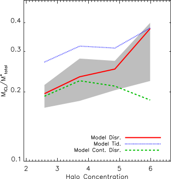
Figure 3: Left Panel: Fraction of ICL as a function of halo concentration for the 53 haloes from our simulations with $M_{200}[M_{\odot}/h]>10^{14}$. Halo concentration is defined as $c_{200}=r_{s}/r_{200}$, where $r_{s}$ is the characteristic scale obtained by fitting the halo density profile to a NFW profile. Right Panel: Fraction of ICL as a function of halo formation time, defined as the time when the main progenitor of the halo has acquired 50 per cent of its final mass. Predictions from different models are shown by lines of different colour, as indicated in the legend. The gray shaded region shows the 20th and 80th percentile of the distribution found for model Disr.

As discussed above, the ICL fraction predicted by our models does not vary as a function of the host halo mass but exhibits a relatively large halo-to-halo scatter, particularly at the group mass scale. The natural expectation is that this scatter is largely determined by a variety of mass accretion histories at fixed halo mass. We can address this issue explicitly using our simulations. In Figure 3, we show how the ICL fraction correlates with the halo concentration in the left panel, and with the halo formation time in the right panel. We note that these two halo properties are correlated (see e.g. Giocoli et al. 2012). As usually done in the literature, we have defined the formation time of the halo as the time when its main progenitor has acquired half of its final mass. The concentration has been computed by fitting the density profile of the simulated haloes with a NFW profile (Navarro, Frenk & White 1996). To remove the known correlations between halo mass and concentration/formation time (Bullock et al. 2001; Neto et al. 2007; Power et al. 2012), we consider in Figure 3 only the 53 haloes from our simulations with $M_{200}[M_{\odot}/h]>10^{14}$. As in previous figures, we show the dispersion (20th and 80th percentiles of the distribution) only for model Disr. The other two models exhibit a similar scatter.

The figure shows that, for the halo mass range considered, the ICL fraction increases with increasing concentration/formation time for models Disr. and Tid while remaining approximately constant for model Cont. Strip. Therefore, for models Disr. and Tid., large part of the scatter seen in Figure 2 for haloes in the mass range considered can be explained by a range of dynamical histories of haloes. Haloes that ‘formed’ earlier (those were also more concentrated) had more time to strip stars from their satellite galaxies or accumulate ICL through accretion of smaller systems, and therefore end up with a larger fraction of ICL. For model Cont. Strip., no clear trend as a function of either halo concentration or halo formation time is found. This happens because, contrary to the other two models, the way we model stellar stripping in the Cont. Strip. model does not introduce any dependence on halo concentration. In this model, the amount of stellar mass stripped from satellite galaxies depends only on properties computed at the time of accretion (i.e. mass ratio, circularity of the orbit). In contrast, in models Disr. and Tid., the stripping efficiency is computed considering the instantaneous position of satellite galaxies. Dynamical friction rapidly drags more massive satellites (those contributing more to the ICL) towards the centre, where stripping becomes more efficient. Our results show that equation 7 is not able to capture this variation, although it is by construction included in the simulations used to calibrate our model.

For lower mass haloes, there is no clear correlation between ICL fraction and the two halo properties considered. This is in part due to the fact that, as we will see in the next section, the bulk of the ICL forms very late - later than the typical formation time of low-mass haloes. In this low-mass range, large part of the scatter in the ICL fraction is driven by the fact that these haloes typically contain relatively few massive galaxies, that are those contributing the bulk of the ICL (see next section). So it is the scatter in the accretion of single massive galaxies that drives the relatively large dispersion seen in Figure 2 for haloes with mass smaller than $10^{14}\,{\rm M}_{\odot}$. We have explicitly verified this by considering the 20 per cent haloes in this mass range with the highest and lowest ICL fractions. We find that for those haloes that have larger ICL components, this has been contributed by a few relatively massive satellite galaxies (stellar mass larger than $10^{10}\,{\rm M}_{\odot}$). In contrast, the ICL in haloes with lower ICL fractions was contributed by less massive satellite galaxies.

Figure 4: Fraction of ICL as a function of the number of satellites within $R_{200}$, with mass larger than the thresholds indicated in the legend. The figure refers to haloes in the mass range $10^{13.4}<M_{200}[M_{\odot}h^{-1}]<10^{13.6}$, and to the model Disr.

In a recent work, Purcell et al. (2007) study how the fraction of ICL varies over a wide range of halo masses (from that of spiral galaxies like our Milky Way to that of massive galaxy clusters) using an analytic model for subhalo infall and evolution, and empirical constraints to assign a stellar mass to each accreted subhalo. In their model, the stellar mass associated with a subhalo is assumed to be added to the diffuse component when a certain fraction of the subhalo dark matter mass has been stripped by tidal interaction with the parent halo. In particular, their fiducial model assumes that disruption of the stellar component starts when 20 per cent of the subhalo mass remains bound. Over the range of halo masses sampled in our study, Purcell et al. (2007) predict a weak increase of the ICL fraction, from $\sim 20$ per cent for haloes of mass $\sim 10^{13}\,{\rm M}_{\odot}$ to about 30 per cent for massive galaxy clusters of mass $\sim 10^{15}\,{\rm M}_{\odot}$. One specific prediction of their model is that the fraction of ICL correlates strongly with the number of surviving satellite galaxies. As they explain, this correlation arises from the fact that haloes that acquired their mass more recently had relatively less time to disrupt the subhaloes they host, and therefore have less ICL.

We analyse the same correlation within our models in Figure 4. This shows the ICL fraction as a function of the number of satellite galaxies within $R_{200}$ for haloes in the mass range $10^{13.4}<M_{200}[M_{\odot}h^{-1}]<10^{13.6}$, and for model Disr.. Lines of different style correspond to different mass cuts, as indicated in the legend. The figure shows that, when considering all galaxies with stellar mass larger than $10^{9}\,{\rm M}_{\odot}$, no significant trend is found between the ICL fraction and the corresponding number of surviving satellite galaxies (this number ranges between $\sim 20$ and $\sim 45$ for this stellar mass cut). When increasing the stellar mass cut, the number of surviving satellites decreases (as expected), and a trend appears in the sense that larger ICL fractions are measured for lower numbers of surviving satellites. Similar trends are found for model Tid., while for model Cont. Strip. no trend is found between the number of surviving satellites and the ICL fraction, for any mass cut used.

6 Formation of the ICL

In this section, we take advantage of our models to analyse when the bulk of the ICL forms, which galaxies provide the largest contribution to it, what is the fraction of ICL that has been accreted from other haloes during the hierarchical growth of clusters, and what fraction is instead contributed from the merger channel.

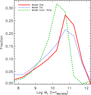
Figure 5: Fraction of the ICL component as a function of the galaxy stellar mass that contributed to it. In the case of model Disr., the galaxy stellar mass on the x-axis refers to the mass that the satellite has before its disruption. For model Cont. Strip., it corresponds to the satellite mass before stripping takes place. For model Tid., both cases can occur.

In Figure 5, we show the contribution to the ICL from galaxies with different stellar mass. For model Disr., the galaxy mass on the x-axis corresponds to that of the satellite right before its disruption, while for model Cont. Strip. it corresponds to the satellite mass before stripping takes place. For model Tid., both cases can occur. The distributions shown in Figure 5 represent the average obtained considering all haloes in our simulated sample. When considering haloes in different mass bins, the distributions are similar but, as expected, they shift towards lower stellar masses for lower mass haloes.

The figure shows that the bulk of the ICL comes from galaxies with stellar masses $\sim 10^{11}\,{\rm M}_{\odot}$ for models Disr. and Tid., and $\sim 10^{10.3}\,{\rm M}_{\odot}$ for model Cont. Strip. In particular, we find that for models Disr. and Tid., about 26 per cent of the ICL is contributed by galaxies with stellar mass in the range $10^{10.75}-10^{11.25}M_{\odot}$. About 68 per cent comes from satellites more massive than $10^{10.5}M_{\odot}$, while dwarf galaxies contribute very little. For model Cont. Strip., almost all the ICL mass ($\sim 90$ per cent of it) comes from satellites with mass in the range $10^{9}-10^{11}M_{\odot}$. The merger channel does not affect significantly the distributions shown.

The result discussed above can be easily understood in terms of dynamical friction: the most massive satellites decay through dynamical friction to the inner regions of the halo on shorter time-scales than their lower mass counterparts. Tidal forces are stronger closer to the halo centre, so that the contribution to the ICL from stripping and/or disruption of massive galaxies is more significant than that from low mass satellites. The latter tend to spend larger fractions of their lifetimes at the outskirts of their parent halo, where tidal stripping is weaker.

The differences between predictions from models Disr. and Tid. and those from model Cont. Strip. are due to a combination of different effects. On one side, model Cont. Strip. uses a different merger time prescription that leads to significantly shorter merger times than in models Disr. and Tid. This is particularly important for the most massive satellites that have the shortest merger times. In addition, while in models Disr. and Tid. satellite galaxies can be completely destroyed, stripping takes place in a more continuous and smooth fashion in model Cont. Strip. These two effects combine so that the largest contribution to the ICL in this model comes from ‘intermediate’ mass satellites that orbit long enough in the cluster potential to be affected significantly by stellar stripping.

Similar results have been found in other studies. In the work by Purcell et al. (2007) mentioned above, the ICL on the cluster mass scale is largely produced by the disruption of satellite galaxies with mass $\sim 10^{11}\,{\rm M}_{\odot}$. In a more recent work, Martel et al. (2012) combine N-body simulations with a subgrid treatment of galaxy formation. They find that about 60 per cent of the ICL in haloes more massive than $\sim 10^{14}\,{\rm M}_{\odot}$ is due to the disruption of galaxies with stellar mass in the range $6\times 10^{8}-3\times 10^{10}\,{\rm M}_{\odot}$. Their results are close to predictions from our model Cont. Strip., with an enhanced contribution of intermediate-mass galaxies with respect to the other two models discussed in this study and results from Purcell et al. (2007). However, in agreement with our results and those from Purcell et al. (2007), they also find that the contribution from low-mass galaxies to the ICL is negligible, though they dominate the cluster galaxy population in number.

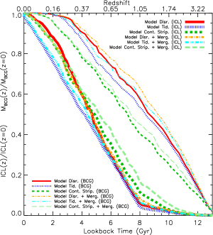
Figure 6: Fraction of stellar mass in ICL as a function of the look-back time, normalized to the amount of ICL at present (thick lines of different style and color). Thinner lines show the evolution in the stellar mass of the main progenitor of BCGs as a function of lookback time.

The analysis discussed above answers the question on ‘which’ galaxies contribute (most) to the ICL component. We can now take advantage of results from our models to ask ‘when’ the ICL is produced. We address this issue in Figure 6 that shows the ICL fraction (normalized to the total amount of ICL measured at present) as a function of cosmic time, for all different prescriptions used in this study (thick lines of different colour and style). The cosmic evolution of the ICL component is compared with the evolution of the stellar mass in the main progenitor of the corresponding BCGs, shown as thin lines.

In agreement with previous studies both based on simulations (Willman et al. 2004; Murante et al. 2007) and on analytic or semi-analytic models (Conroy et al. 2007; Monaco et al. 2006), we find that the bulk of the ICL forms relatively late, below $z=1$. Models Disr. and Tid. predict very similar ICL growth histories, while in model Cont. Strip. the ICL formation appears to be anticipated with respect to the other two models. At redshift $\sim 1$, less than 10 per cent of the ICL was already formed in models Disr. and Tid. If the merger channel for the formation of the ICL is switched on in these models, the ICL fraction formed at the same redshift increases to $\sim 15-20$ per cent. As explained earlier, the importance of the merger channel is enhanced in model Cont. Strip. The figure also shows that the ICL grows slower than the mass in the main progenitor of the BCG down to $z\sim 1$, i.e. at a lookback time of $\sim 8$ Gyr. Below this redshift, the ICL component grows much faster than the BCG, with more than 80 per cent of the total ICL mass found at z=0 being formed during this redshift interval.

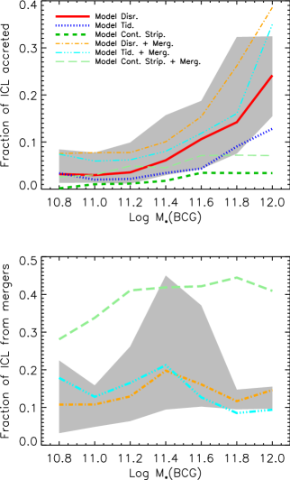
Figure 7: Top panel: fraction of accreted ICL as a function of the BCG stellar mass. Bottom panel: fraction of ICL contributed by the merger channel as a function of the BCG stellar mass. The grey shaded region shows the 20th and 80th percentiles of the distribution measured for model Disr. The other models exhibit similar dispersions.

We now want to quantify what is the fraction of ICL that is accreted onto the cluster during its hierarchical growth. As explained in Section 3, the amount of ICL associated with a central galaxy can increase through three channels:

• stripping of satellite galaxies orbiting in the same parent halo;

• mergers, if this particular channel is switched on;

• accretion of the ICL component that is associated with new galaxies infalling onto the cluster during its assembly history or with satellite galaxies (i.e. when a Type 1 becomes a Type 2 galaxy in model Disr. or when a Type 1 is stripped for the first time in models Tid. and Cont. Strip).

In the following, we define the ‘accreted’ component as the ICL fraction that is coming through the third channel described above. The contribution from this component is shown in the top panel of Figure 7 as a function of the stellar mass of the BCG. In models Disr. and Tid., the fraction of the accreted component increases from a few per cent for the least massive BCGs in our sample to $\sim 13-25$ per cent for the most massive BCGs, in case the merger channel is off. For model Cont. Strip., the increase as a function of the BCG stellar mass is less pronounced, and the fraction of accreted ICL is always below 10 per cent even in the case the merger channel is on.

The bottom panel of Figure 7 quantifies the amount of ICL that comes from the merger channel. If this channel is switched on, as we have seen in the left panel of Figure 2, the ICL fraction increases in each model. We note that the amount of ICL that comes from this channel cannot be inferred precisely by comparing each model in Figure 2 with its counterpart including the merger channel, because it affects slightly the merger times of galaxies. The contributions to the ICL coming from mergers are shown in the bottom panel of Figure 7, and have been stored using the three prescriptions used in this study with the merger channel on. We find that in models Disr. and Tid. the merger channel contributes to $\sim 15$ per cent of the total ICL. For model Cont. Strip., the contribution from mergers is significantly larger, ranging from $\sim 30$ per cent for the least massive BCGs in our sample, to $\sim 40$ per cent for the most massive ones.

7 ICL and BCG properties

We now focus on the relation between the ICL and the main properties of BCGs, such as stellar mass and luminosity, and analyse how these are affected by the inclusion of our prescriptions for the formation of the ICL.

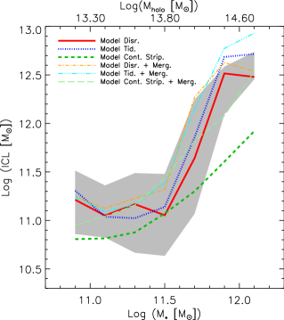
Figure 8: Stellar mass in the ICL component as a function of the BCGs stellar mass. Lines of different style and colour correspond to different models, as indicated in the legend. The grey shaded region shows the 20th and 80th percentiles of the distribution obtained for model Disr.

In Figure 8 we show the relation between the mass in the ICL component and the stellar mass of the BCG. As expected, more massive BCGs reside in haloes that host a more conspicuous ICL component. For models Disr. and Tid., the correlation is strong for BCGs more massive than $\sim 3\times 10^{11}\,{\rm M}_{\odot}$, while it is very weak for less massive central galaxies. Model Cont. Strip. predicts a weaker correlation over the mass range explored, and a significantly lower mass in the ICL component with respect to the other two models when the merger channel is off.

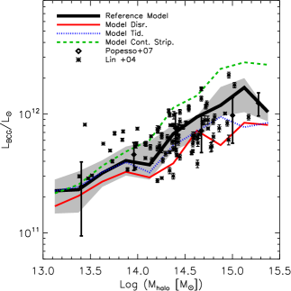
Figure 9: Relation between the BCG luminosity in K-band and the cluster mass ($M_{200}$). Black stars with error bars show the observational measurements by Lin & Mohr (2004), while black diamonds with error bars are observational measurements by Popesso et al. (2007). The thick black solid line shows predictions from our reference model (DLB07), while thinner lines of different style show predictions from the models including our different prescriptions for the formation of the ICL. The grey shaded region shows the 20th and 80th percentiles of the distribution obtained for the reference model. Our other models have comparable scatter.

Figure 9 shows the luminosity of the BCG in the K-band as predicted by our models as a function of the halo mass. Model predictions are compared with observational measurements by Lin & Mohr (2004) and Popesso et al. (2007). It is worth recalling that our model luminosities are ‘total’ luminosities, that are difficult to measure observationally: Popesso et al. (2007) use SDSS ‘model magnitudes’, while Lin & Mohr (2004) use elliptical aperture magnitudes corresponding to a surface brightness of $\mu_{K}=20\,\rm{mag/arcsec^{2}}$, and include an extra correction of 0.2 mag to get their ‘total magnitudes’. Our reference model is in very good agreement with both sets of observational data. Models Disr. and Tid. predict slightly lower luminosities than our reference model, as a consequence of the reduced accretion of stellar mass from satellites (either because part of these are destroyed - model Disr., or because they are stripped - model Tid.). Model Cont. Strip. predicts luminosities of central galaxies brighter than those measured by Popesso et al., on the cluster mass scale. This is due to the fact that, as mentioned earlier, merger times are shorter in this model, which increases the stellar mass and the luminosity of the BCGs by accretion of (massive) satellites.

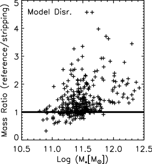
Figure 10: Ratio between the stellar mass of BCGs in the reference model and the corresponding value in model Disr., as a function of the stellar mass in the reference model.

Surprisingly, we find that also in models Disr. and Tid. a small fraction of the BCGs are brighter (more massive) than in the reference model. Naively, we do not expect this to be possible as the only effect of our prescriptions should be that of reducing the stellar mass of satellite galaxies by stripping or disruption. In Figure 10, we show the ratio between the BCG stellar mass in the reference model and the corresponding stellar mass in model Disr., as a function of the former quantity. The Figure shows that the majority of the BCGs are more massive in the reference model, but about 23 per cent of the BCGs in our sample are actually more massive when we switch on our prescription for the disruption of satellite galaxies. If we additionally switch on the merger channel for the formation of the ICL, the fraction of BCGs that are more massive in model Disr. than in the reference model reduces to about 10 per cent. Model Tid. behaves in a similar way (the corresponding fractions are 28 and 9 per cent, respectively). Model Cont. Strip., as also evident from Figure 9 behaves differently. In this model, about half (42 per cent) of the BCGs are more massive than in the reference model, with this fraction reducing to about 26 per cent when the merger channel is switched on. While in model Disr. (and Tid.) the effect seems to be limited to the less massive BCGs (those with stellar mass lower than $\sim 10^{11.5}M_{\odot}$), in model Cont. Strip. this happens for BCGs of any mass.

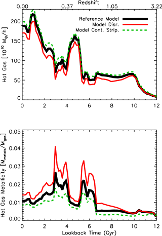
Figure 11: Top panel: Mass in the hot component available at each redshift, for a BCG that is found to be more massive in model Disr. (and less massive in model Cont. Strip.) than in the reference model. Bottom panel: hot gas metallicity at each redshift. Results are shown for different models, as indicated in the legend.

In order to understand this finding, we have analysed the evolution of the stellar mass, mass gained through mergers, and cooling rate for a number of the BCGs that are more massive in model Disr. than in the reference model. We have found that in all cases, the reason for the increased mass of the BCGs can be traced back to a more efficient cooling rate. In order to illustrate this, we show in Figure 11 a representative example. The top panel shows the amount of hot gas available for cooling onto the main progenitor of the BCG, up to $z\sim 3$, while the bottom panel shows the corresponding metallicity. Results are shown for the reference model, and for our models Disr. and Cont. Strip. (model Tid. behaves similarly to the reference model). For this particular BCG, the evolution of both the hot gas content and that of its metallicity in model Disr. follow very closely the evolution in the reference model. At $z\sim 1.5$, the metallicity of the hot gas in model Disr. becomes higher than in the reference model, and this causes a significant increase in the cooling rate. In turn, the more efficient cooling determines an increase in the star formation, and therefore of the final BCG stellar mass. The behaviour is different in model Cont. Strip. where the metallicity of the hot gas actually falls below the corresponding value in the reference model. As we have explained earlier, for this particular model we have used a different implementation of the merger times which introduces a net decrease in the merger time of satellite galaxies. This more rapid merger rates causes about half of the BCGs to be more massive in model Cont. Strip. than in the reference model.

The difference in the hot gas metallicity of the BCG between model Disr. and Cont. Strip. is due to a different metal content of the gas accreted from satellite galaxies. We recall that when a satellite galaxy is destroyed (or stripped), its stellar mass goes to the ICL while its gaseous content, including the corresponding metals, go to the hot gas component associated with the central galaxy. In model Cont. Strip., stripping is a continuous process that starts as soon as a galaxy becomes a satellite. In addition, in this model the formation of the ICL component starts earlier than in the other models, as shown in Figure 6. In this case, the gas that is removed from satellites tends to dilute the metallicity of the hot gas component. In model Disr. (as well as in model Tid.), the formation of the ICL starts a bit later, and satellite galaxies are more massive than in model Cont. Strip. (and therefore also more metal rich - see Figure 5), so that their disruption tends on average to increase the metal content of the hot gas component.

8 ICL metallicity

From the observational viewpoint, little is known about the stellar populations of the ICL component. Using I-band HST data, Durrell et al. (2002) compared the brightness of Virgo ICL red giant branch (RGB) stars to that of RGB stars in a metal-poor dwarf galaxies, and estimated an age for the ICL population older than $\sim 2$ Gyr, and a relatively high metallicity ($-0.8\lesssim[{\rm Fe/H}]\lesssim-0.2$). Williams et al. (2007) use HST observations of a single intra-cluster field in the Virgo Cluster and find that the field is dominated by low-metallicity stars ($[{\rm M/H}]\lesssim-1.$) with ages older than $\sim 10$ Gyr. However, they find that the field contains stars of the full range of metallicities probed ($-2.3\leq[{\rm M/H}]\leq 0.0$), with the metal-poor stars exhibiting more spatial structure than metal-rich stars, suggesting that the intra-cluster population is not well mixed. Using long-slit spectra and measuring the equivalent width of Lick indices, Coccato et al. (2011) find that most of the stars in the dynamically hot halo of NGN3311 (the BCG in the Hydra I cluster) are old and metal-poor ($[{\rm Z/H}]\sim-0.35$).

In this section, we present predictions of our models concerning in particular the metallicity of the ICL component. We recall that our model adopts an instantaneous recycling approximation for chemical enrichment. In particular, we assume that a constant yield of heavy elements is produced per solar mass of gas converted into stars, and that all metals are instantaneously returned to the cold phase. Metals are then exchanged between the different phases proportionally to the mass flows. When a satellite galaxy is stripped of some fraction of its stars (or destroyed), a proportional fraction (or all) of the metals are also moved from the satellite stars into the ICL.

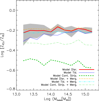
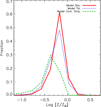
Figure 12: Left panel: mean metallicity of the ICL component as a function of halo mass. Predictions from different models are shown using lines of different style and colour. The shaded gray region shows the 20th and 80th percentiles of the distribution obtained for model Disr. Right panel: average distribution of the metallicities of the stars in the ICL component for all haloes in our sample.

The left panel of Figure 12 shows the median metallicity of the ICL component, as a function of halo mass, for our different prescriptions. The grey shaded region shows the 20th and 80th percentiles of the distribution found for model Disr. (the other models exhibit similar dispersions). In our models, the ICL metallicity does not vary significantly as a function of the halo mass. Assuming $Z_{\odot}=0.02$, the average metallicity of the ICL in models Disr. and Tid. is $\sim 0.63Z_{\odot}$, while for model Cont. Strip. the ICL metallicity is significantly lower ($\sim 0.32-0.50Z_{\odot}$). This is a consequence of the fact that the galaxies contributing to the ICL are on average less massive (and more metal-poor) than those that contribute to the ICL in models Disr. and Tid. (see Figure 5). In the right panel of Figure 12, we show the average metallicity distribution of stars in the ICL component for all haloes in our sample. As a consequence of the results shown in Figure 5, model Cont. Strip. predicts a distribution shifted towards lower metallicities, with a peak at $\sim 0.4Z_{\odot}$. Models Disr. and Tid. predict distributions that are less broad and peaked at higher metallicities.

Our model results are therefore qualitatively consistent with observational measurements by Williams et al. (2007), with most of the stars in the ICL having sub-solar metallicity but covering a relatively wide range.

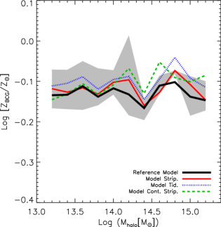
Figure 13: BCG stellar metallicity as a function of halo mass. Lines of different style and colour correspond to the different prescriptions used in our study, as indicated in the legend. The thick solid black line shows predictions from our reference model.

Figure 13 shows the BCG metallicity predicted by the different models used in our study, as a function of the halo mass. The figure shows that all models predict very similar metallicities for the BCGs, of about $0.74\,Z_{\odot}$. Predictions are close to those of the reference model (thick solid black line). On average, stellar stripping slightly increases the BCG metallicity, particularly in model Tid. This happens because the most massive galaxies receive less low-metallicity stars from satellite galaxies whose masses (and metal contents) are reduced because of stellar stripping.

Our results confirm findings by De Lucia & Borgani (2012) who show that the model mass-metallicity relation is offset low with respect to the observational measurements at the massive end. In particular, the observed BCG metallicities (similar to those of the most massive galaxies) are expected to be at least 0.2-0.3 dex larger (von der Linden et al. 2007; Loubser et al. 2009). Figure 13 shows that the inclusion of a model for the formation of the ICL component does not significantly improve this disagreement. More in general, we find that our modelling of the formation of the ICL component does not significantly affect the predicted mass-metallicity relation. This is in apparent contrast with findings by Henriques & Thomas (2010) who claim that the introduction of satellite disruption is sufficient to bring the stellar metallicities of the most massive galaxies in agreement with the observational data. We note that Henriques & Thomas (2010) use the same reference model adopted in our study and employ a Monte Carlo Markov Chain parameter estimation technique to constrain the model with the K-band luminosity function, the B-V colours, and the black hole-bulge mass relation. The ‘best fit’ model found by Henriques & Thomas (2010) includes a model for tidal stripping of the satellite galaxies, but also adopts different parameters with respect to the reference model, in particular for the supernovae feedback and gas recycling process (see their Table 2). We therefore argue that, as discussed also in De Lucia & Borgani (2012), that stellar stripping cannot provide alone the solution to the problem highlighted above, and that modifications of the star formation and feedback processes are required.

9 Discussion and conclusions

In this work, we build upon the semi-analytic model presented in De Lucia & Blaizot (2007, DLB07) to describe the generation of intra-cluster light (ICL). We include different implementations for modelling the formation of the diffuse ICL. In particular, we consider: (i) a model that assumes the stellar component of satellite galaxies can be affected only after their parent dark matter substructures are stripped below the resolution limit of the simulation (Disruption model); (ii) a model that accounts for stellar stripping also from satellites sitting in distinct dark matter subhaloes, and based on a simple estimate of the tidal radius (Tidal Radius model); and (iii) a model based on a fitting formula derived from a suite of numerical simulations aimed to study the evolution of a disk galaxy within the global tidal field of a group environment (Villalobos et al. 2012, Continuous Stripping model). In addition, we have also considered the relaxation processes acting during galaxy-galaxy mergers by simply assuming that 20 per cent of the stellar mass of the merging satellite gets unbound and ends-up in the ICL component associated with the remnant galaxy. In our implementations, the bulk of the ICL is produced through tidal stripping and disruption of the satellite galaxies, with the merger channel contributing only for a minor fraction.

The reference model we have used is known to over-predict the abundance of galaxies with mass below $\sim 10^{10}\,{\rm M}_{\odot}$ (Fontanot et al. 2009; Guo et al. 2011). The inclusion of a model for stellar stripping of satellite galaxies alleviates this problem, but does not solve it. In a recent work, Budzynski et al. (2012) use a catalogue of groups and clusters from SDSS DR7 in the redshift range $0.15\leq z\leq 0.4$ and compare the galaxy number density profiles with predictions from the same reference model used in our study. They show that the model follows very well the observational measurements but in the very central regions (within $\sim 0.2R_{500}$), where the predicted profile is steeper than observational measurements. The inclusion of stellar stripping would improve the agreement with data in this region where the tidal field is stronger and galaxies are more likely to be stripped. However, the same comparison with the data by Lin et al. (2004) would lead to an opposite conclusion. This suggests that the uncertainty on the density profiles in the inner region is probably too large to put strong constraints on stripping models.

As we discuss below, we find that the dominant contribution to the ICL formation comes from stripping and/or disruption of massive satellites so that the excess of intermediate to low-mass galaxies does not affect significantly our results. In our Cont. Strip. model, we use a different prescription for merger times with respect to that employed in the reference model and in the other two models considered (see Section 3.3). As a consequence, merger times are on average shorter than in the other models which result in an under-prediction of massive satellites. We note that recent work by Villalobos et al. (2013) has pointed out that the dynamical friction formula used in our Continuous Stripping model (Boylan-Kolchin et al. (2008)) under-estimate merger times at higher redshift. Implementing their proposed modification would make merger times longer in this model, making results more similar to the other two models. We have explicitly tested (by adding a fudge factor that increases again the merger times so as to bring the predicted mass function in agreement with observations) that this does not affect significantly the results presented in this work.

A number of recent studies have focused on the formation of the ICL, using both hydrodynamical numerical simulations (e.g. Murante et al. 2007; Puchwein et al. 2010; Rudick et al. 2006), and analytic models based on subhalo infall and evolution (e.g. Purcell et al. 2007; Watson et al. 2012). Less work on the subject has been carried out using semi-analytic models of galaxy formation, but for basic predictions in terms of how the fraction of ICL depends on the parent halo mass (Monaco et al. 2006; Somerville et al. 2008; Guo et al. 2011).

Our models predict an ICL fraction that varies between $\sim 20$ and $\sim 40$ per cent (depending on the particular implementation adopted), with no significant trend as a function of the parent halo mass. Results are in qualitative agreement with observational data, in particular on the cluster mass scale. We note, however, that the ICL fractions predicted by our models depend on the resolution of the simulations: for a set of simulations that use a particle mass one order of magnitude larger than that adopted in the high resolution runs used in our study, the predicted ICL fractions increase by  30-40 per cent. We stress that both the data and the model predictions exhibit a relatively large halo-to-halo scatter. On the cluster mass scale, we find that the scatter is largely due to a variety of mass accretion histories at fixed halo mass, as argued by Purcell et al. (2007): objects that formed earlier (that were also more concentrated) had more time to strip stars from their satellite galaxies or accumulate ICL through accretion of smaller systems. On group scale, where the predicted scatter is very large, we do not find any clear correlation between ICL fraction and halo concentration or formation time. We show that, on these scales, large part of the scatter is driven by individual accretion events of massive satellites. The (albeit weak) correlation between the ICL fraction and concentration on the cluster mass scale can be tested observationally, e.g. by measuring the ICL fraction and concentration for system lying in a relatively narrow halo mass range.

Our models predict that the ICL forms very late, below redshift $z\sim 1$, in agreement with previous analysis based on hydrodynamical numerical simulations (e.g. Murante et al. 2007). About 5 to 25 per cent of the diffuse light has been accreted during the hierarchical growth of dark matter haloes, i.e. it is associated with new galaxies falling onto the haloes during their assembly history. In addition, we find that the bulk of the ICL is produced by the most massive satellite galaxies, $M\sim 10^{10-11}\,{\rm M}_{\odot}$, in agreement with recent findings based on N-body simulations (Martel et al. 2012) and analytic models (Purcell et al. 2007). Low-mass galaxies ($M_{*}<10^{9}M_{\odot}$) contribute very little to the ICL in terms of mass, although they dominate in terms of number. This is a natural consequence of dynamical friction triggering the generation of the ICL: the most massive satellites approach the inner cluster regions faster than their less massive counterparts. Close to the cluster centre, tidal forces are stronger, increasing the stripping efficiency. In contrast, small satellites spend most of their time in the outer regions where tidal stripping is weaker.

Since most of the ICL is produced by tidal stripping of massive satellites, this component is found to have a metallicity that is similar to that of these galaxies. Our model predictions are in qualitative agreement with observations, with most of the stars in the diffuse component having on average sub-solar metallicities (but covering a relatively large range). We also find that the mean metallicity of the ICL is approximately constant as a function of halo mass, and exhibit a relatively small halo-to-halo scatter. In contrast, Purcell et al. (2008) predict a weak increase of the ICL metallicity with increasing halo mass, over the same halo mass range considered in our study. Finally, we show that the inclusion of a model for tidal stripping of satellite galaxies does not significantly affect the predicted mass-metallicity relation, and only slightly increases the metallicity of the most massive galaxies. For all models, these galaxies have stellar metallicities significantly lower than observed (see also De Lucia & Borgani 2012). Future and more detailed observations focused e.g. on age and metallicity of the ICL component will help constraining our models and understanding the physical mechanisms driving the formation of this important stellar component.

Appendix A Numerical Convergence

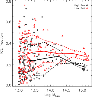
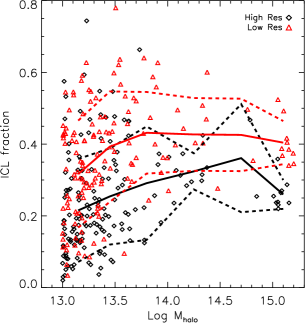
Figure 14: Left Panel: ICL fraction predicted by the Disruption model as a function of halo mass, for haloes in the high resolution set used in this paper (black lines and symbols), and the corresponding low-resolution version (red lines and symbols). Dashed lines show the one sigma dispersion, while solid lines correspond to the mean. Right Panel: same as the left panel, but for the Tidal Radius model.

In the left panel of Figure 14 we show the ICL fraction as a function of cluster mass, as predicted by the Disruption model applied to two sets of simulations: a set with high-resolution (the one we used in the paper), and the corresponding low-resolution set where the same initial conditions were used for each halo but the particle mass adopted is one order of magnitude larger. The ICL fraction appears to be systematically higher in the low-resolution set over all the halo mass range considered, with the difference being more significant on cluster scale. This is due to the fact that, decreasing the resolution, a larger fraction of satellite galaxies are classified as Type 2 and are subject to our stripping model. The effect is weaker in low-mass haloes that have a lower number of satellites galaxies.

We carried out the same convergence test also for Tidal Radius model, and show the corresponding results in the right panel of Figure 14. The ICL fraction is higher in the low-resolution set than in the high resolution set, by about 40 per cent. Due to the constraint given by equation 6, events of stripping of Type 1 satellites are extremely rare in this model, and their contribution to the ICL fraction is lower than 1 per cent over all the halo mass range considered. This means that Type 2 galaxies are the main contributors to the total amount of ICL. The larger fraction of these galaxies in the low-resolution set causes the increase of the ICL fraction, also on group scale, where the increase seems to be more important than it is in Disruption model.

References

- Abadi et al. (2006) Abadi M. G., Navarro J. F., Steinmetz M., 2006, MNRAS, 365, 747
- Arnaboldi et al. (2012) Arnaboldi M., Ventimiglia G., Iodice E., Gerhard O., Coccato L., 2012, A&A, 545, A37
- Benson (2005) Benson A. J., 2005, MNRAS, 358, 551
- Binney & Tremaine (2008) Binney J., Tremaine S., 2008, Galactic Dynamics: Second Edition. Princeton University Press
- Boylan-Kolchin et al. (2008) Boylan-Kolchin M., Ma C.-P., Quataert E., 2008, MNRAS, 383, 93
- Budzynski et al. (2012) Budzynski J. M., Koposov S. E., McCarthy I. G., McGee S. L., Belokurov V., 2012, MNRAS, 423, 104
- Bullock et al. (2001) Bullock J. S., Kolatt T. S., Sigad Y., Somerville R. S., Kravtsov A. V., Klypin A. A., Primack J. R., Dekel A., 2001, MNRAS, 321, 559
- Calcáneo-Roldán et al. (2000) Calcáneo-Roldán C., Moore B., Bland-Hawthorn J., Malin D., Sadler E. M., 2000, MNRAS, 314, 324
- Coccato et al. (2011) Coccato L., Gerhard O., Arnaboldi M., Ventimiglia G., 2011, A&A, 533, A138
- Conroy et al. (2007) Conroy C., Wechsler R. H., Kravtsov A. V., 2007, ApJ, 668, 826
- Contini et al. (2012) Contini E., De Lucia G., Borgani S., 2012, MNRAS, 420, 2978
- De Lucia & Blaizot (2007) De Lucia G., Blaizot J., 2007, MNRAS, 375, 2
- De Lucia & Borgani (2012) De Lucia G., Borgani S., 2012, MNRAS, 426, L61
- De Lucia et al. (2010) De Lucia G., Boylan-Kolchin M., Benson A. J., Fontanot F., Monaco P., 2010, MNRAS, 406, 1533
- Diemand et al. (2005) Diemand J., Madau P., Moore B., 2005, MNRAS, 364, 367
- Dolag et al. (2010) Dolag K., Murante G., Borgani S., 2010, MNRAS, 405, 1544
- Durrell et al. (2002) Durrell P. R., Ciardullo R., Feldmeier J. J., Jacoby G. H., Sigurdsson S., 2002, ApJ, 570, 119
- Feldmeier et al. (2004) Feldmeier J. J., Ciardullo R., Jacoby G. H., Durrell P. R., 2004, ApJ, 615, 196
- Font et al. (2006) Font A. S., Johnston K. V., Bullock J. S., Robertson B. E., 2006, ApJ, 638, 585
- Fontanot et al. (2009) Fontanot F., De Lucia G., Monaco P., Somerville R. S., Santini P., 2009, MNRAS, 397, 1776
- Giocoli et al. (2012) Giocoli C., Tormen G., Sheth R. K., 2012, MNRAS, 422, 185
- Gonzalez et al. (2005) Gonzalez A. H., Zabludoff A. I., Zaritsky D., 2005, ApJ, 618, 195
- Gonzalez et al. (2007) Gonzalez A. H., Zaritsky D., Zabludoff A. I., 2007, ApJ, 666, 147
- Gregg & West (1998) Gregg M. D., West M. J., 1998, Nature, 396, 549
- Guo et al. (2011) Guo Q., White S., Boylan-Kolchin M., De Lucia G., Kauffmann G., Lemson G., Li C., Springel V., Weinmann S., 2011, MNRAS, 413, 101
- Henriques & Thomas (2010) Henriques B. M. B., Thomas P. A., 2010, MNRAS, 403, 768
- Jiang et al. (2008) Jiang C. Y., Jing Y. P., Faltenbacher A., Lin W. P., Li C., 2008, ApJ, 675, 1095
- Katz & White (1993) Katz N., White S. D. M., 1993, ApJ, 412, 455
- Lin & Mohr (2004) Lin Y.-T., Mohr J. J., 2004, ApJ, 617, 879
- Lin et al. (2004) Lin Y.-T., Mohr J. J., Stanford S. A., 2004, ApJ, 610, 745
- Liu et al. (2010) Liu L., Yang X., Mo H. J., van den Bosch F. C., Springel V., 2010, ApJ, 712, 734
- Loubser et al. (2009) Loubser S. I., Sánchez-Blázquez P., Sansom A. E., Soechting I. K., 2009, MNRAS, 398, 133
- Martel et al. (2012) Martel H., Barai P., Brito W., 2012, ApJ, 757, 48
- Matthews et al. (1964) Matthews T. A., Morgan W. W., Schmidt M., 1964, ApJ, 140, 35
- McGee & Balogh (2010) McGee S. L., Balogh M. L., 2010, MNRAS, 403, L79
- Mihos (2004) Mihos J. C., 2004, Clusters of Galaxies: Probes of Cosmological Structure and Galaxy Evolution, p. 277
- Mo et al. (1998) Mo H. J., Mao S., White S. D. M., 1998, MNRAS, 295, 319
- Monaco et al. (2006) Monaco P., Murante G., Borgani S., Fontanot F., 2006, ApJ, 652, L89
- Murante et al. (2004) Murante G., Arnaboldi M., Gerhard O., Borgani S., Cheng L. M., Diaferio A., Dolag K., Moscardini L., Tormen G., Tornatore L., Tozzi P., 2004, ApJ, 607, L83
- Murante et al. (2007) Murante G., Giovalli M., Gerhard O., Arnaboldi M., Borgani S., Dolag K., 2007, MNRAS, 377, 2
- Navarro et al. (1996) Navarro J. F., Frenk C. S., White S. D. M., 1996, ApJ, 462, 563
- Neto et al. (2007) Neto A. F., Gao L., Bett P., Cole S., Navarro J. F., Frenk C. S., White S. D. M., Springel V., Jenkins A., 2007, MNRAS, 381, 1450
- Popesso et al. (2007) Popesso P., Biviano A., Böhringer H., Romaniello M., 2007, A&A, 464, 451
- Power et al. (2012) Power C., Knebe A., Knollmann S. R., 2012, MNRAS, 419, 1576
- Puchwein et al. (2010) Puchwein E., Springel V., Sijacki D., Dolag K., 2010, MNRAS, 406, 936
- Purcell et al. (2007) Purcell C. W., Bullock J. S., Zentner A. R., 2007, ApJ, 666, 20
- Purcell et al. (2008) Purcell C. W., Bullock J. S., Zentner A. R., 2008, MNRAS, 391, 550
- Read et al. (2006) Read J. I., Pontzen A. P., Viel M., 2006, MNRAS, 371, 885
- Rudick et al. (2006) Rudick C. S., Mihos J. C., McBride C., 2006, ApJ, 648, 936
- Rudick et al. (2011) Rudick C. S., Mihos J. C., McBride C. K., 2011, ApJ, 732, 48
- Somerville et al. (2008) Somerville R. S., Hopkins P. F., Cox T. J., Robertson B. E., Hernquist L., 2008, MNRAS, 391, 481
- Sommer-Larsen (2006) Sommer-Larsen J., 2006, MNRAS, 369, 958
- Springel et al. (2005) Springel V., White S. D. M., Jenkins A., Frenk C. S., Yoshida N., Gao L., Navarro J., Thacker R., Croton D., Helly J., Peacock J. A., Cole S., Thomas P., Couchman H., Evrard A., Colberg J., Pearce F., 2005, Nature, 435, 629
- Springel et al. (2001) Springel V., White S. D. M., Tormen G., Kauffmann G., 2001, MNRAS, 328, 726
- Toledo et al. (2011) Toledo I., Melnick J., Selman F., Quintana H., Giraud E., Zelaya P., 2011, MNRAS, 414, 602
- Tormen et al. (1997) Tormen G., Bouchet F. R., White S. D. M., 1997, MNRAS, 286, 865
- Trentham & Mobasher (1998) Trentham N., Mobasher B., 1998, MNRAS, 293, 53
- Villalobos et al. (2012) Villalobos Á., De Lucia G., Borgani S., Murante G., 2012, ArXiv e-prints
- Villalobos et al. (2013) Villalobos Á., De Lucia G., Weinmann S., Borgani S., Murante G., 2013, ArXiv e-prints
- von der Linden et al. (2007) von der Linden A., Best P. N., Kauffmann G., White S. D. M., 2007, MNRAS, 379, 867
- Watson et al. (2012) Watson D. F., Berlind A. A., Zentner A. R., 2012, ArXiv e-prints
- Williams et al. (2007) Williams B. F., Ciardullo R., Durrell P. R., Vinciguerra M., Feldmeier J. J., Jacoby G. H., Sigurdsson S., von Hippel T., Ferguson H. C., Tanvir N. R., Arnaboldi M., Gerhard O., Aguerri J. A. L., Freeman K., 2007, ApJ, 656, 756
- Willman et al. (2004) Willman B., Governato F., Wadsley J., Quinn T., 2004, MNRAS, 355, 159
- Zibetti (2008) Zibetti S., 2008, in Davies J. I., Disney M. J., eds, IAU Symposium Vol. 244 of IAU Symposium, Statistical Properties of the IntraCluster Light from SDSS Image Stacking. pp 176–185
- Zibetti et al. (2005) Zibetti S., White S. D. M., Schneider D. P., Brinkmann J., 2005, MNRAS, 358, 949
- Zwicky (1937) Zwicky F., 1937, ApJ, 86, 217
- Zwicky (1952) Zwicky F., 1952, PAPS, 64, 242