Galaxies on FIRE (Feedback In Realistic Environments): Stellar Feedback Explains Cosmologically Inefficient Star Formation

Abstract

We present a series of high-resolution cosmological simulations${}^{\ref{foot:movie}}$ of galaxy formation to $z=0$, spanning halo masses $\sim 10^{8}-10^{13}\,M_{\sun}$, and stellar masses $\sim 10^{4}-10^{11}\,M_{\sun}$. Our simulations include fully explicit treatment of the multi-phase ISM & stellar feedback. The stellar feedback inputs (energy, momentum, mass, and metal fluxes) are taken directly from stellar population models. These sources of feedback, with zero adjusted parameters, reproduce the observed relation between stellar and halo mass up to $M_{\rm halo}\sim 10^{12}\,M_{\sun}$. We predict weak redshift evolution in the $M_{\ast}-M_{\rm halo}$ relation, consistent with current constraints to $z>6$. We find that the $M_{\ast}-M_{\rm halo}$ relation is insensitive to numerical details, but is sensitive to feedback physics. Simulations with only supernova feedback fail to reproduce observed stellar masses, particularly in dwarf and high-redshift galaxies: radiative feedback (photo-heating and radiation pressure) is necessary to destroy GMCs and enable efficient coupling of later supernovae to the gas. Star formation rates agree well with the observed Kennicutt relation at all redshifts. The galaxy-averaged Kennicutt relation is very different from the numerically imposed law for converting gas into stars, and is determined by self-regulation via stellar feedback. Feedback reduces star formation rates and produces reservoirs of gas that lead to rising late-time star formation histories, significantly different from halo accretion histories. Feedback also produces large short-timescale variability in galactic SFRs, especially in dwarfs. These properties are not captured by common “sub-grid” wind models.

1 Introduction

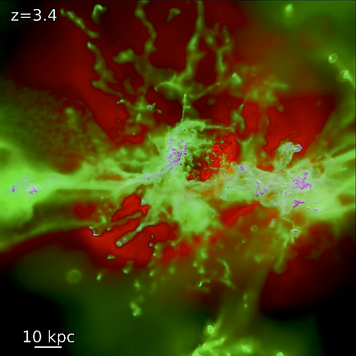
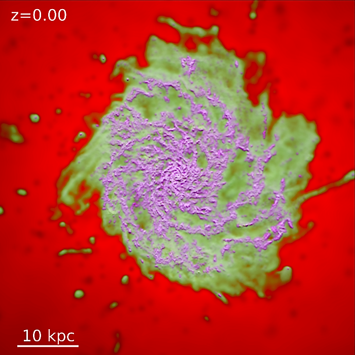
Figure 1: Gas in a representative simulation of a Milky Way-mass halo (m12i in Table 1). Image shows the projected gas density, log-weighted ($\sim 4\,$dex stretch). Magenta shows cold molecular/atomic gas ($T<1000\,$K). Green shows warm ionized gas ($10^{4}\lesssim T\lesssim 10^{5}\,$K). Red shows hot gas ($T\gtrsim 10^{6}\,$K).${}^{\ref{foot:gas.coloring}}$ Each image shows a box centered on the main galaxy. Left: Box $200\,$kpc (physical) on a side at high redshift. The galaxy has undergone a violent starburst, leading to strong outflows of hot and warm gas that have blown away much of the surrounding IGM (even outside the galaxy). Note that the “filamentary” structure of cool gas in the IGM is clearly affected by the outflows. Right: Near present-day, with a $\sim 50\,$kpc box. A more relaxed, well-ordered disk has formed, with molecular gas tracing spiral structure, and a halo enriched by diffuse hot outflows.

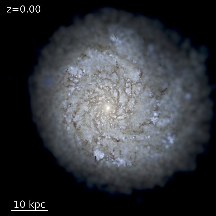
Figure 2: Stars in the m12i simulation at $z\sim 0$, in a box $50\,$kpc on a side near present-time. Image is a mock $u/g/r$ composite. The disk is approximately face-on, and the spiral structure is visible. (The image uses STARBURST99 to determine the SED of each star particle given its known age and metallicity, then ray-traces the line-of-sight flux following Hopkins et al. (2005), attenuating with a MW-like reddening curve with constant dust-to-metals ratio for the abundances at each point.)

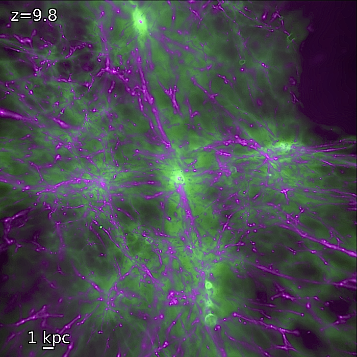
Figure 3: Gas, as Fig. 1, for a dwarf galaxy (m10 in Table 1). Top: $40\,$kpc (physical) box, at high redshift. Bottom: $20\,$kpc box at intermediate redshift. Strong outflows are still present, though they are more spherical, because the galaxy halo is itself small and embedded within a much larger filament.

It is well-known that feedback from stars is a critical, yet poorly-understood, component of galaxy formation. Within galaxies, star formation is observed to be inefficient in both an instantaneous and an integral sense.

Instantaneously, the Kennicutt-Schmidt (KS) relation implies gas consumption timescales of $\sim 50$ dynamical times (Kennicutt, 1998), while the total fraction of GMC mass converted into stars is only a few percent (Zuckerman & Evans, 1974; Williams & McKee, 1997; Evans, 1999; Evans et al., 2009). Without strong stellar feedback, however, gas inside galaxies cools efficiently and collapses on a dynamical time, predicting order-unity star formation efficiencies on all scales (Hopkins et al., 2011; Tasker, 2011; Bournaud et al., 2010; Dobbs et al., 2011; Krumholz et al., 2011; Harper-Clark & Murray, 2011).

In an integral sense, without strong stellar feedback, gas in cosmological models cools rapidly and inevitably turns into stars, predicting galaxies with far larger masses than are observed (e.g. Katz et al., 1996; Somerville & Primack, 1999; Cole et al., 2000; Springel & Hernquist, 2003b; Kereš et al., 2009, and references therein). Decreasing the instantaneous star formation efficiency does not eliminate this integral problem: the amount of baryons in real galactic disks is much lower than that predicted in models absent strong feedback (essentially, the Universal baryon budget; see White & Frenk, 1991; Kereš et al., 2009). Constraints from intergalactic medium (IGM) enrichment require that many of those baryons must have entered galaxy halos and disks at some point to be enriched, before being expelled (Aguirre et al., 2001; Pettini et al., 2003; Songaila, 2005; Martin et al., 2010). Galactic super-winds with mass-loading $\dot{M}_{\rm wind}$ of many times the star formation rate (SFR) are therefore generally required to reproduce observed galaxy properties (e.g. Oppenheimer & Davé, 2006). Such winds have been observed ubiquitously in local and high-redshift star-forming galaxies (Martin, 1999, 2006; Heckman et al., 2000; Newman et al., 2012; Sato et al., 2009; Chen et al., 2010; Steidel et al., 2010; Coil et al., 2011).

However, until recently, numerical simulations have been unable to produce winds with large-mass loading factors from an a priori model (let alone the correct scalings of wind mass-loading with galaxy mass or other properties), nor to simultaneously predict the instantaneous inefficiency of star formation within galaxies. This is particularly true of models which invoke only energetic feedback via supernovae (SNe), which is efficiently radiated in the dense gas where star formation actually occurs (see e.g. Guo et al., 2010; Powell et al., 2011; Brook et al., 2011; Nagamine, 2010; Bournaud et al., 2011, and references therein). More recent simulations, using higher resolution and invoking stronger feedback prescriptions, have seen strong winds, but have generally found it necessary to include simplified prescriptions for “turning off cooling” in the SNe-heated gas and/or include some adjustable parameters representing “pre-SNe” feedback (see Governato et al., 2010; Macciò et al., 2012; Teyssier et al., 2013; Stinson et al., 2013; Agertz et al., 2013). This is physically motivated since feedback processes other than SNe – protostellar jets, HII photoionization, stellar winds, and radiation pressure – both occur and are critical in suppressing star formation in dense gas, as well as “pre-processing” gas prior to SNe explosions so that SNe occur at densities where thermal heating can have much larger effects (Evans et al., 2009; Hopkins et al., 2011; Tasker, 2011; Lopez et al., 2011; Stinson et al., 2013; Kannan et al., 2013).

And in fact, there have been many studies with enormously higher resolution (enough to evolve each star explicitly) and a full treatment of the radiation-magnetohydrodynamics and time dependence of these multiple feedback mechanisms. Because of computational limitations, however, these have necessarily been restricted to very small systems, either single molecular clouds/star clusters (e.g. Krumholz et al., 2007, 2011; Offner et al., 2009, 2011; Harper-Clark & Murray, 2011; Bate, 2012), or the “first stars” (e.g. Wise et al., 2012; Pawlik et al., 2013; Muratov et al., 2013). But these studies, without exception, have found that the non-linear interaction of the feedback mechanisms above – especially the dual roles of HII photoionization and radiation pressure in concert with SNe – is absolutely critical to explain the generation of large local outflows, the self-regulation of star formation, and the shape of the stellar initial mass function.

Despite these breakthroughs, given limited resolution and the complexity of the baryonic physics, many cosmological models have treated galactic wind generation and the inefficiency of star formation in a tuneable, “sub-grid” fashion. This is not to say that the models have not tremendously improved our understanding of galaxy formation! They have demonstrated that stellar feedback can plausibly lead to (globally) inefficient star formation, constrained the parameter space of allowed feedback models, made predictions for the critical role of outflows and recycling in enriching the IGM, provided possible baryonic solutions to apparent dark matter “problems” (e.g. Pontzen & Governato, 2012), demonstrated the need for “early” feedback from radiative mechanisms beyond SNe alone, and generally created the framework for our interpretation of observations. However, with wind models often relying on adjustable parameters, the integrated efficiency of star formation in galaxies is to some extent tuned “by hand” and the predictive power is inherently limited. This is particularly true for studies of gas in the circum-galactic medium (CGM), a current area of much observational progress – measurements of the CGM are sensitive to the phase structure of the gas, which is not faithfully represented in models which simply “turn off” hydrodynamics or cooling, or mimic strong feedback via pure thermal energy injection or “particle kicks” (see e.g. Hummels et al., 2013, for an explicit demonstration of this).

Accurate treatment of star formation and galactic winds ultimately requires realistic treatment of the stellar feedback processes that maintain the multi-phase ISM. Motivated by this philosophy (and building on the studies with single-star resolution), in Hopkins et al. (2011) (Paper I) and Hopkins et al. (2012d) (Paper II), we developed a new set of numerical models to follow stellar feedback on scales from sub-GMC star-forming regions through galaxies. These simulations include the energy, momentum, mass, and metal fluxes from stellar radiation pressure, HII photo-ionization and photo-electric heating, SNe Types I & II, and stellar winds (O-star and AGB). Critically, the feedback is directly tied to the young stars, with the energetics and time-dependence taken from stellar evolution models. In our previous work, we showed, in isolated galaxy simulations, that these mechanisms produce a quasi-steady ISM in which GMCs form and disperse rapidly, with phase structure, turbulence, and disk and GMC properties in good agreement with observations (for various comparisons, see Narayanan & Hopkins, 2012; Hopkins et al., 2012b, a, 2013c). In Paper I, Hopkins et al. (2013d), and Hopkins et al. (2013a) we showed that this leads naturally to “instantaneously” inefficient SF (predicting the KS-law), regulated self-consistently by feedback and independent of the numerical prescription for star formation in very dense gas. In Hopkins et al. (2012c) (Paper III) and Hopkins et al. (2013b) we showed that the same feedback models reproduce the galactic winds invoked in previous semi-analytic and cosmological simulations, and that the combination of multiple feedback mechanisms is critical to produce massive, multi-phase galactic winds.

However, our simulations have thus far been limited to idealized studies of isolated galaxies and galaxy mergers. These previous calculations thus cannot follow accretion from or interaction of outflows with the IGM, realistic galaxy merger histories, and many other important processes. In this paper, the first of a series, we present the FIRE (Feedback In Realistic Environments) simulations: a suite of fully cosmological “zoom-in” simulations developed to study the role of feedback in galaxy formation. To test the models and understand feedback in a wide range of environments, we study a wide range in galaxy halo and stellar mass (as opposed to focusing just on MW-like systems), and follow evolution fully to $z=0$. Our suite of calculations includes several of the highest-resolution galaxy formation simulations that have been run to $z=0$. Our simulations utilize a significantly improved numerical implementation of SPH (which has resolved historical discrepancies with grid codes), as well as the full physical models for feedback and ISM physics introduced and tested in Paper I-Paper III. Here, we explore the consequences of stellar feedback for the inefficiency of star formation, perhaps the most basic consequence of stellar feedback for galaxy formation. In companion papers, we will investigate the properties of outflows and their interactions with the IGM, the effect of those outflows on dark matter structure, the differences between numerical methods in treating feedback, the role of feedback in determining galaxy structure, and many other open questions.

In § 2-4, we describe our methodology. § 2 describes the initial conditions for the simulations; § 3 outlines the implementation of the key baryonic physics of cooling, star formation, and feedback (a much more detailed description is given in Appendix A); § 4 briefly describes the improvements in the numerical method compared to past work (again, more details are in Appendix B). And in Appendix C we test and compare these algorithms with higher-resolution simulations of isolated (non-cosmological) galaxies.

We describe our results in § 5. We examine the predicted galaxy stellar masses (§ 5.1), and how this depends on both numerical algorithms (§ 5.3) and feedback physics (§ 5.4), as well as how it compares to previous theoretical work (§ 5.5). We show that the treatment of feedback physics overwhelmingly dominates these results, and discuss the distinct roles of multiple independent feedback mechanisms. We also explore the predictions for the Kennicutt-Schmidt relation (§ 5.6), the shape of galaxy star formation histories (§ 5.7), the star formation “main sequence” (§ 5.8), and the “burstiness” of star formation (§ 5.9). We summarize our important conclusions and discuss future work in § 6.

2 Initial Conditions & Galaxy Properties

The simulations presented here are a series of fully cosmological “zoom-in” simulations of galaxy formation; some images of the gas and stars in representative stages are shown in Figs. 1-3. The technique is well-studied; briefly, a large cosmological box is simulated at low resolution to $z=0$, and then the mass within and around halos of interest at that time is identified, traced back to the starting redshift, and the Lagrangian region containing this mass is re-initialized at much higher resolution (with gas added) for the ultimate simulation (Porter, 1985; Katz & White, 1993).

We consider a series of systems with different masses. Table 1 describes the initial conditions. All simulations begin at redshifts $\sim 100-125$, with fluctuations evolved using perturbation theory up to that point.

Table 1: Simulation Initial Conditions 

Name $M_{\rm halo}^{0}$ $m_{b}$ $\epsilon_{b}$ $m_{dm}$ $\epsilon_{dm}$ Merger Notes [$h^{-1}\,M_{\sun}$] [$h^{-1}\,M_{\sun}$] [$h^{-1}$pc] [$h^{-1}\,M_{\sun}$] [$h^{-1}$pc] History m09 1.9e9 1.8e2 1.0 8.93e2 20 normal isolated dwarf m10 0.8e10 1.8e2 2.0 8.93e2 20 normal isolated dwarf m11 1e11 5.0e3 5.0 2.46e4 50 quiescent – m12v 5e11 2.7e4 7.0 1.38e5 100 violent several $z<2$ mergers m12q 1e12 5.0e3 7.0 1.97e5 100 late merger – m12i 1e12 3.5e4 10 1.97e5 100 normal large ($\sim 10\,R_{\rm vir}$) box m13 1e13 2.6e5 15 1.58e6 150 normal “small group” mass

	Parameters describing the initial conditions for our simulations (units are physical):
(1) Name: Simulation designation.
(2) $M_{\rm halo}^{0}$: Approximate mass of the $z=0$ “main” halo (most massive halo in the high-resolution region).
(3) $m_{b}$: Initial baryonic (gas and star) particle mass in the high-resolution region, in our highest-resolution simulations.
(4) $\epsilon_{b}$: Minimum baryonic gravity/force softening (minimum SPH smoothing lengths are comparable or smaller). Recall, force softenings are adaptive (mass resolution is fixed); for more details see Appendix B.
(3) $m_{dm}$: Dark matter particle mass in the high-resolution region, in our highest-resolution simulations.
(4) $\epsilon_{dm}$: Minimum dark matter force softening (fixed in physical units at all redshifts).

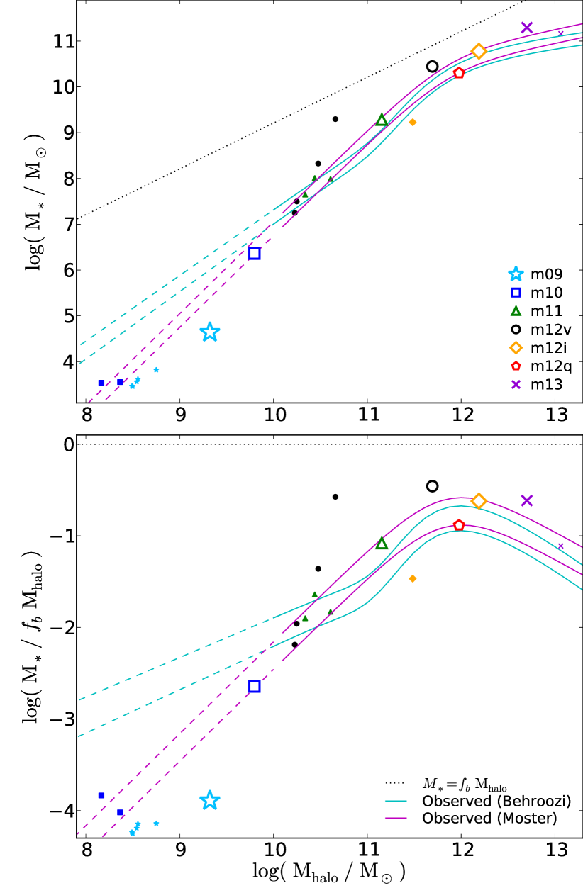
Figure 4: Galaxy stellar mass-halo mass relation at $z=0$. Top: $M_{\ast}(M_{\rm halo})$. Bottom: $M_{\ast}$ relative to the Universal baryon budget of the halo ($f_{b}\,M_{\rm halo}$). Each simulation (points) from Table 1 is shown; large point denotes the most massive halo in each box. We compare the relation if all baryons became stars ($M_{\ast}=f_{b}\,M_{\rm halo}$; dotted) and the observationally inferred relationship as determined in Moster et al. (2013, magenta) and Behroozi et al. (2012, cyan) (dashed lines denote extrapolation beyond the observed range).${}^{\ref{foot:moster.behroozi.halo.defns}}$ The agreement with observations is excellent at $M_{\rm halo}\lesssim 10^{13}\,M_{\sun}$, including dwarf though MW-mass galaxies. We stress that there are zero adjusted parameters here: stellar feedback, with known mechanisms taken from stellar population models, is sufficient to explain galaxy stellar masses at/below $\sim L_{\ast}$.

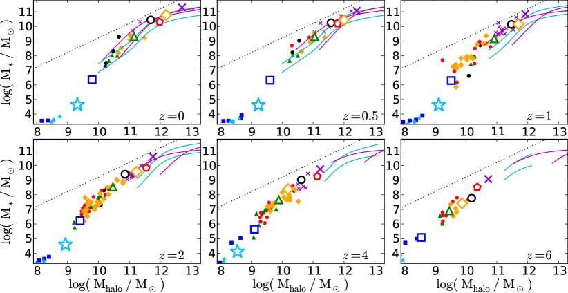
Figure 5: $M_{\ast}-M_{\rm halo}$ relation as Fig. 4 (points follow the legend therein), at different redshifts. Observational constraints are also shown at each redshift (each pair of lines shows the $\pm 1\,\sigma$ fit to the observations at that redshift). With no tuned parameters, the simulations predict $M_{\ast}-M_{\rm halo}$ and, by extension, the stellar MF and galaxy clustering, at all $z$. Redshift evolution in $M_{\ast}-M_{\rm halo}$ is weak, with the sense that low-mass dwarfs become higher-$M_{\ast}$, leading to a steeper faint-end galaxy MF, in agreement with constraints from reionization (see Kuhlen & Faucher-Giguère, 2012, and references therein).

The specific halos we re-simulate are chosen to represent a broad mass range and be “typical” in most properties (e.g. sizes, formation times, and merger histories) relative to other halos of the same $z=0$ mass. The simulations m09 and m10 are constructed using the methods from Onorbe et al. (2013); they are isolated dwarfs. Simulations m11, m12q, m12i, and m13 are chosen to match a subset of initial conditions from the AGORA project (Kim et al., 2013), which will enable future comparisons with a wide range of different codes. These are chosen to be somewhat quiescent merger histories, but lie well within the typical scatter in such histories at each mass (and each has several major mergers). Simulation m12v, for contrast, is chosen to have a relatively violent merger history (several major mergers since $z\sim 2$), and is based on the initial conditions studied in Kereš & Hernquist (2009) and Faucher-Giguère & Kereš (2011).

In each case, the resolution is scaled with the simulated mass, so as to achieve the optimal possible force and mass resolution. It is correspondingly possible to resolve much smaller structures in the low-mass galaxies. The critical point is that in all our simulations with mass $<10^{13}\,M_{\sun}$, we resolve the Jeans mass/length of gas in the galaxies, corresponding to the size/mass of massive molecular cloud complexes. This is necessary to resolve a genuine multi-phase ISM and for our ISM feedback physics to be meaningful. Fortunately, because most of the mass and star formation in GMCs in both observations (Evans, 1999; Blitz & Rosolowsky, 2005) and simulated systems (Paper II) is concentrated in the most massive GMCs, the resolution studies in Paper I-Paper II confirm that resolving small molecular clouds makes little difference. We refer interested readers to Paper II for a detailed discussion of the scales that must be resolved for feedback to operate appropriately, but note here that all our simulations are designed to be approximately comparable to the “high-resolution” simulations of isolated galaxies and the ISM in Paper I-Paper II, within the range of resolution where the results in those studies (star formation rates, wind outflow rates, GMC lifetimes, etc.) were numerically converged (unfortunately, it is not possible to evolve cosmological simulations to $z=0$ with the “ultra-high” sub-pc resolution therein).

In terms of the Jeans mass/length of the galaxies, our resolution is broadly comparable between different simulations. Our worst resolution in units of the Jeans length/mass occurs in the more massive galaxies at late times, when they are relatively gas poor, and so (despite the large total galaxy mass) the Jeans length can become relatively small. Every galaxy identified in this paper contains at least $\gg 10^{5}$ bound particles.

We adopt a “standard” flat $\Lambda$CDM cosmology with $h\approx 0.7$, $\Omega_{{\rm M}}=1-\Omega_{\Lambda}\approx 0.27$, and $\Omega_{b}\approx 0.046$ for all runs.

3 Baryonic Physics

The simulations here use the physical models for star formation and stellar feedback developed and presented in a series of papers studying isolated galaxies (Hopkins et al., 2012c, 2013a, b, a), adapted for fully cosmological simulations. We summarize their properties below, but refer to Appendix A for a more detailed explanation and list of improvements. Readers interested in further details (including resolution studies and a range of tests of the specific numerical methodology) should see Paper I & Paper II.

3.1 Cooling

Gas follows an ionized+atomic+molecular cooling curve from $10-10^{10}\,$K, including metallicity-dependent fine-structure and molecular cooling at low temperatures, and high-temperature ($\gtrsim 10^{4}\,$K) metal-line cooling followed species-by-species for 11 separately tracked species. At all times, we tabulate the appropriate ionization states and cooling rates from a compilation of CLOUDY runs, including the effect of the photo-ionizing background, accounting for gas self-shielding. Photo-ionization and photo-electric heating from local sources are accounted for as described below.

3.2 Star Formation

Star formation is allowed only in dense, molecular, self-gravitating regions above $n>n_{\rm crit}$ ($n_{\rm crit}=100\,{\rm cm^{-3}}$ for our primary runs, but we also tested from $\sim 10-1000\,{\rm cm^{-3}}$). This threshold is much higher than that adopted in most “zoom-in” simulations of galaxy formation (the high value allows us to capture highly clustered star formation). We follow Krumholz & Gnedin (2011) to calculate the molecular fraction $f_{\rm H_{2}}$ in dense gas as a function of local column density and metallicity, and allow SF only from molecular gas. We also follow Hopkins et al. (2013d) and restrict star formation to gas which is locally self-gravitating, i.e. has $\alpha\equiv\delta v^{2}\,\delta r/G\,m_{\rm gas}(<\delta r)<1$ on the smallest available scale ($\delta r$ being our force softening or smoothing length). This forms stars at a rate $\dot{\rho}_{\ast}=\rho_{\rm mol}/t_{\rm ff}$ (i.e. $100\%$ efficiency per free-fall time); so that the galaxy and even kpc-scale star formation efficiency is not set by hand, but regulated by feedback (typically at much lower values). Because of this, in Paper I, Paper II, and Hopkins et al. (2013d) we show that the galaxy structure and SFR are basically independent of the small-scale SF law, density threshold (provided it is high), and treatment of molecular chemistry.

3.3 Stellar Feedback

Once stars form, their feedback effects are included from several sources. Every star particle is treated as a single stellar population, with a known age, metallicity, and mass. Then all feedback quantities (the stellar luminosity, spectral shape, SNe rates, stellar wind mechanical luminosities, metal yields, etc.) are tabulated as a function of time directly from the stellar population models in STARBURST99, assuming a Kroupa (2002) IMF.

(1) Radiation Pressure: Gas illuminated by stars feels a momentum flux $\dot{P}_{\rm rad}\approx(1-\exp{(-\tau_{\rm UV/optical})})\,(1+\tau_{\rm IR})\,L_{\rm incident}/c$ along the optical depth gradient, where $1+\tau_{\rm IR}=1+\Sigma_{\rm gas}\,\kappa_{\rm IR}$ accounts for the absorption of the initial UV/optical flux and multiple scatterings of the re-emitted IR flux if the region between star and gas particle is optically thick in the IR (see Appendix A). We assume that the opacities scale linearly with gas metallicity.

(2) Supernovae: We tabulate the SNe Type-I and Type-II rates from Mannucci et al. (2006) and STARBURST99, respectively, as a function of age and metallicity for all star particles and stochastically determine at each timestep if an individual SNe occurs. If so, the appropriate mechanical luminosity and ejecta momentum is injected as thermal energy and radial momentum in the gas within a smoothing length of the star particle, along with the relevant mass and metal yield (for all followed species). When the Sedov-Taylor phase is not fully resolved, we account for the work done by hot gas inside the unresolved cooling radius (converting the appropriate fraction of the SNe energy into momentum). We discuss this in detail in Appendix A, but emphasize that it is particularly important that SNe momentum not be neglected in massive halos whose mass resolution $\sim 10^{4}\,M_{\sun}$ is much larger than the ejecta mass of a single SNe.

(3) Stellar Winds: Similarly, stellar winds are assumed to shock locally and so we inject the appropriate tabulated mechanical power $L(t,\,Z)$, wind momentum, mass, and metal yields, as a continuous function of age and metallicity into the gas within a smoothing length of the star particles. The integrated mass fraction recycled in winds (including both fast winds from young stars and slow AGB winds) and SNe is $\sim 0.3$.

(4) Photo-Ionization and Photo-Electric Heating: Knowing the ionizing photon flux from each star particle, we ionize each neighboring neutral gas particle (provided there are sufficient photons, given the gas density, metallicity, and prior ionization state), moving outwards until the photon budget is exhausted; this alters the heating and cooling rates appropriately. The UV fluxes are also used to determine photo-electric heating rates following Wolfire et al. (1995).

Extensive numerical tests of the feedback models are presented in Paper II.

4 Simulation Numerical Details

All simulations are run using a newly developed version of TreeSPH which we refer to as “P-SPH” (Hopkins, 2013), in the code GIZMO. This adopts the Lagrangian “pressure-entropy” formulation of the SPH equations developed in Hopkins (2013); this eliminates the major differences between SPH, moving mesh, and grid (adaptive mesh) codes, and resolves the well-known issues with fluid mixing instabilities in previously-used forms of SPH (e.g. Agertz et al., 2007; Sijacki et al., 2012). The gravity solver is a heavily modified version of the GADGET-3 code (Springel, 2005); but GIZMO also includes substantial improvements in the artificial viscosity, entropy diffusion, adaptive timestepping, smoothing kernel, and gravitational softening algorithm, as compared to the “previous generation.” These are all described in detail in Appendix B.

We emphasize that our version of SPH has been tested extensively and found to give good agreement with analytic solutions as well as well-tested grid codes on a broad suite of test problems. Many of these are presented in Hopkins (2013). This includes Sod shock tubes; Sedov blastwaves; wind tunnel tests (radiative and adiabatic, up to Mach $\sim 10^{4}$); linear sound wave propagation; oscillating polytropes; hydrostatic equilibrium “deformation”/surface tension tests (Saitoh & Makino, 2013); Kelvin-Helmholtz and Rayleigh-Taylor instabilities; the “blob test” (Agertz et al., 2007); super-sonic and sub-sonic turbulence tests (from Mach $\sim 0.1-10^{3}$); Keplerian gas ring, disk shear, and shearing shock tests (Cullen & Dehnen, 2010); the Evrard test; the Gresho-Chan vortex; spherical collapse tests; and non-linear galaxy formation tests. For additional tests showing the improvements relative to previous-generation SPH, see Hu et al. (2014). Since it is critical for the problems addressed here that a code be able to handle high dynamic range situations, the numerical method and parameters such as SPH “neighbor number” were not modified for these tests individually, but are similar to what we use in our production runs in this paper.

In Appendix B, we note that we have explicitly tested many of the purely numerical elements of the gravity and hydrodynamic solvers in the simulations shown here: for example, whether to use adaptive or fixed gravitational softenings, the choice of SPH smoothing kernel, and the timestepping algorithm. However we do not discuss these in the main text because they produce extremely small ($\lesssim 10\%$-level) differences in the quantities plotted in this paper.

5 Results

5.1 Galaxy Masses as a Function of Redshift

Fig. 4 plots the $z=0$ stellar mass-halo mass relation for our main set of simulations from Table 1 (highest-resolution, with all physics enabled). Note that although each high-resolution region at $z=0$ contains one “primary” halo (the focus of that region), there are several smaller-mass, independent halos also in that region. We therefore identify and plot all such halos. We exclude those halos that are outside the high-resolution region (more than $1\%$ mass-contaminated by low-resolution particles; although varying this between $0.5-10\%$ makes little difference to our comparisons here) or insufficiently resolved ($<0.01$ times the primary halo mass, or with $<10^{5}$ dark matter particles). We also exclude subhalos/satellite galaxies.

The known sources of stellar feedback we include, with no adjustment, automatically reproduce a relation between galaxy stellar and halo mass consistent with the observations from $M_{\rm halo}\sim 10^{7}-10^{13}\,M_{\sun}$. Specifically, the distribution of points for all $M_{\rm halo}\leq 10^{12}\,M_{\sun}$ is statistically consistent (in a $\chi^{2}$ sense) with having been drawn from the Moster et al. (2013) curve; if we allow for the observed scatter ($\sim 0.15\,$dex at $\sim 10^{12}\,M_{\sun}$, the width between the plotted lines, increasing to $\sim 0.3\,$dex at the lowest observed masses) then all our primary galaxies lie within the $2\,\sigma$ scatter.

Despite the fact that this relation implies a non-uniform (and even non-monotonic) efficiency of star formation as a function of galaxy mass, we do not need to invoke different physics or distinct parameters at different masses. This is particularly impressive at low masses, where the integrated stellar mass must be suppressed by factors of $\sim 1000$ relative to the Universal baryon fraction. Unfortunately, at high masses ($>10^{13}\,M_{\sun}$), the large Lagrangian regions (hence large number of required particles) limit the resolution we can achieve; we have experimented with some low-resolution test runs which appear to produce overly massive galaxies, but higher-resolution studies are required to determine if that owes to a need for additional physics or simply poor numerical resolution.

Interestingly, the scatter in $M_{\ast}$ at fixed $M_{\rm halo}$ may decrease weakly with mass, from $\sim 0.5$ dex in dwarf galaxies ($M_{\rm halo}\lesssim 10^{10}\,M_{\sun}$) to $\sim 0.1-0.2$ dex in massive ($\sim L_{\ast})$ galaxies. But given the limited number of halos we study here, further investigation allowing more diverse merger/growth histories is needed.

Fig. 5 shows the $M_{\ast}-M_{\rm halo}$ relation at various redshifts. At each $z$, we compare with observationally constrained estimates of the $M_{\ast}-M_{\rm halo}$ relation. Implicitly, if they agree in $M_{\ast}(M_{\rm halo})$, our models are consistent with the observed stellar MF (given, of course, the limited statistics by which we are “sampling” the MF). At high redshifts, the halos we simulate are of course lower-mass, so eventually we have no high-mass galaxies; this limits the extent to which our results can be compared to observations above $z\sim 2$.

5.2 Other (Basic) Galaxy Properties

We wish to focus here on galaxy masses and star formation histories. Companion papers (in preparation) will examine the galaxy morphologies and other observables in more detail. It is important, when studying those properties, to construct a meaningful comparison (e.g. using the same methods and wavelengths observed), and this is non-trivial. Moreover, it is by no means obvious that these properties are as robust to numerical details as the galaxy stellar masses (discussed further below), and it is completely outside the scope of this paper to fairly explore those dependencies.

That said, we can briefly note the basic properties of the specific simulations in Table 1 at $z=0$, with the caveat that these may not be robust to changes in either the initial conditions (the particular halo simulated) or our numerical methods. Morphologically, at $z=0$, run m09 resembles an ultrafaint dwarf; m10 a thick, but rotating dwarf irregular; and m11 a more “fluffy” dwarf spheroidal. Runs m12v, m12q, m12i produce bulge+disk systems, with m12v showing a prominent bulge at all times $z\lesssim 2$; m12q is more disk-dominated until a late major merger at $z<0.5$ destroys the disk; and run m12i produces a stellar disk with little bulge. Run m13 is totally bulge-dominated. Each galaxy has an approximately flat rotation curve outside of the central couple kpc; those with $M_{\ast}<10^{10}$ slowly rise with radius to $V_{\rm max}$, and the more massive systems are flat to within the central $\sim$ kpc, except for m12v (where the compact bulge leads to a central-kpc spike at $\sim 250\,{\rm km\,s^{-1}}$). The galaxy sizes, measured as the half-stellar mass effective radii, are $(0.3,\,0.52,\,3.5,\,2.8,\,3.2,\,4.2,\,4.8)\,{\rm kpc}$ for (m09, m10, m11, m12v, m12q, m12i, m13), consistent with the observed stellar size-mass relation (Shen et al., 2003; Wolf et al., 2010).

5.3 (Lack of) Dependence on Numerical Methods

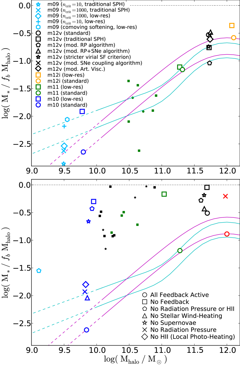
Figure 6: $M_{\ast}-M_{\rm halo}$ relation at $z=0$, as Fig. 4. Top: Simulations with different numerical parameters: we show the effects of varied resolution, artificial viscosity, and the algorithmic implementation of feedback. We also compare a completely different version of SPH (with a different set of hydrodynamic equations), which is known to differ significantly in certain idealized hydrodynamic test problems. These have little effect on our predictions. Bottom: Effect of physical variation in stellar feedback properties. We compare runs with no stellar feedback, with no supernovae (but stellar winds, radiation pressure, and photo-ionization heating included), or with no radiative feedback (radiation pressure and local HII-heating). “No feedback” runs generally predict $M_{\ast}\sim f_{b}\,M_{\rm halo}$, in severe conflict with the observations.${}^{\ref{foot:nofb.lowmhalo}}$ Removing radiative or SNe feedback also produce order-of-magnitude too-large stellar masses. The non-linear combination of feedback mechanisms (not any one in isolation) is critical to drive winds and regulate galaxy masses.

In Fig. 6 we investigate how the $M_{\ast}-M_{\rm halo}$ relation depends on numerical parameters and feedback. First we repeat Fig. 4 for simulations with different purely numerical parameters. These can and do, indeed, have significant quantitative effects – they can easily shift the predicted stellar masses by factors $\sim 2-3$. However, we stress that they do not qualitatively change our conclusions.

Modest changes in resolution (our “low-resolution” runs correspond to one power of two step in spatial resolution, and a corresponding factor of $2^{3}=8$ change in mass resolution) lead to significant, but not order-of-magnitude, changes in $M_{\ast}$: generally we obtain larger $M_{\ast}$ by factors of $\sim 1.5$ at high masses ($M_{\rm halo}\gtrsim 10^{11}\,M_{\sun}$) and $\sim 2-3$ at the lowest masses ($M_{\rm halo}<10^{10}\,M_{\sun}$) at lower resolution, owing to a combination of (a) artificially enhanced mixing and thus cooling of diffuse gas, since ISM phases are less well-resolved, and (b) the fact that the coupling of feedback energy and momentum is necessarily spread over larger mass elements. If we downgrade our resolution more substantially – by a factor of $\sim 100$ in mass, or $>10$ in spatial scale (i.e. using the $>100\,$pc spatial resolution which is typical of most previous cosmological simulations), the results diverge more substantially: galaxy masses at $z\sim 0$ are a factor of $\sim 3-5$ higher at high masses and $\sim 10$ higher at low masses. This makes sense, because at that resolution, we simply cannot meaningfully resolve even the most massive structures in the ISM.

Some of our numerical tests are not plotted here because their effects are not significant. We have, for example, re-run several simulations with twice and five times larger dark matter softening lengths (same baryonic softening); using or de-activating adaptive gravitational softenings (which ensure there are always $\sim 100$ neighbor particles in the softening kernel); varying the number of SPH “neighbors” in the hydrodynamic kernel and number of SPH particles to which energy and momentum are coupled; using a single timestep or Strang-split integration scheme in the code; varying the Courant factor of the hydrodynamic solver; changing the order of operator-splitting for the cooling and feedback steps; or forcing equal vs. allowing separate gravitational softenings for baryons and dark matter. These produce very small ($<10\%$) differences. We also varied the sizes of the high-resolution “zoom-in” Lagrangian regions of the halos; the results here are insensitive to the region size if we choose sizes $\gtrsim 2\,R_{\rm vir}$ (at the redshift of interest), but the cooling of halo gas and star formation are artificially suppressed if the high-resolution region is much smaller.

Changing the small-scale star formation prescription in the simulations has very little effect on our predictions. This is expected based on all of our previous studies using isolated (non-cosmological) simulations (for explicit examples where we vary the density threshold and instantaneous “efficiency” of star formation in dense gas by factors of $>1000$, as well as the density, temperature, chemical, and virial-state dependence of star formation, see Paper I, Paper II, and Hopkins et al. 2013d). Globally, star formation is feedback-regulated: a certain number of young stars are required to balance gravitational collapse/dissipation, independent of how those stars form. So long as cooling can proceed, they will form (what will change, via this self-regulation, if we change e.g. the density threshold above which stars form, is the amount of gas which “builds up” above that threshold; see Hopkins et al. 2012b). In Fig. 6 we show examples where we vary the density threshold for star formation by factors of $\sim 100$ (producing $<0.2$ dex random/non-systematic changes in stellar mass), or impose a much stricter local virial criterion for star formation (local virial parameter $<0.5$ instead of $1$; producing a $\sim 20\%$ difference in stellar mass); we have also experimented with removing the virial parameter entirely or dividing the instantaneous efficiency of star formation in dense gas by a factor of $100$ (both produce $<10\%$ changes).

We have also investigated different purely algorithmic methods for coupling the same feedback physics. Subtle differences in the algorithmic implementation of feedback have little systematic effect on the stellar mass, provided the same mechanisms are included; however they can only be compared statistically, since the stochastic nature of feedback means that even very subtle changes can produce significant differences in the exact time history of bursts, for example. Of what we have considered, the most important parameter is how we implement the momentum gained during the Sedov-Taylor phase of SNe remnant expansion when the cooling radius is unresolved (see Appendix A). For example, one of the “mod. SNe coupling algorithm” examples changes the particle weights (using a standard SPH kernel weight – effectively mass-weighted in the smoothing kernel – instead of a volumetric weighting) used to determine the coupling of SNe energy and momentum in the kernel. This can have dramatic effects on test problems: for a SNe in an infinitely thin, adiabatic disk with a low-density exterior, a mass-weighting couples all the momentum in the disk plane, instead of the vertical direction (the correct solution). Nevertheless we see this has relatively weak ($\sim 20\%$) effects on the stellar mass and star formation history (in part because, in the average over many SNe over large volumes, all that matters is the total feedback input); however, it can significantly effect the morphological structure of e.g. the dense gas in a thin disk. We have also experimented with different functional forms for the ratio of the SNe energy and momentum coupling (producing small effects). The “mod. RP algorithm” choice discretizes our radiation pressure term (which is usually a continuous force) into intentionally very large ($>500\,{\rm km\,s^{-1}}$) “kicks” (this keeps the same total momentum flux, but makes each such particle “kicked” unbound) – unsurprisingly this suppresses star formation further, but only by a factor of $\sim 3$. In the “mod. RP+SNe” choice we discretize the radiation pressure into smaller kicks ($=5\,{\rm km\,s^{-1}}$) and see this has little effect (as expected). In all cases the results lie within the (rather large) range allowed by observations.

In a companion paper, Kereš et al. (2014) consider the detailed effects of substantial changes to each aspect of our numerical method described in Appendix B. Here, we simply show a few basic comparisons. Considerable attention has recently been paid to differences between the results of grid codes and older SPH methods (such as that in Springel & Hernquist 2002) for certain problems (especially sub-sonic fluid mixing instabilities; see Agertz et al. 2007; Kitsionas et al. 2009; Bauer & Springel 2012; Vogelsberger et al. 2012; Sijacki et al. 2012; Kereš et al. 2012). The numerical method used for our standard simulations has been specifically shown to resolve most of these discrepancies (giving results quite similar to grid codes in test problems); this is verified in Hopkins (2013) for standard test problems and Kereš et al. (2014) for cosmological simulations. However we have re-run some of our simulations using the Springel & Hernquist (2002) formulation of SPH (described in Appendix B), which shows the most pronounced forms of these discrepancies. Despite the known differences between such methods for certain test problems, we find in Fig. 6 (top panel) that it makes little difference for the predicted galaxy masses. The older SPH method gives slightly lower $M_{\ast}(M_{\rm halo})$ (by about $\approx 0.15\,$dex), primarily because cooling of diffuse “hot halo” gas is suppressed by less-efficient mixing. But for this specific question, the effect is quite small compared to the effects of including the appropriate stellar feedback physics. We also show an experiment where adopt an entirely distinct artificial viscosity prescription (see Appendix B for details), which produces negligible differences.

It is important to stress that our conclusion here – that our results depend only weakly on the numerical details – applies to the galaxy stellar masses and other lowest-order, integrated quantities. In future work, we will study other properties of the simulations, such as the galaxy morphologies, which can (and do) depend on some parameters much more sensitively. For example, the modifications to the SNe coupling algorithm described above, which produce very little systematic change in our predicted stellar masses and star formation histories, produce surprisingly large changes to the angular momentum content and thickness of disks in the more massive galaxies.

Finally, we show these results in part to stress, emphatically, that while there are always numerical choices in any code, there has been no “tuning” of these parameters for our study here. Certainly none of these has been “fit” or “adjusted” to match any observations, and all the choices above are held constant across our standard set of simulations, using values calibrated from simple test problems (e.g. Hopkins, 2013).

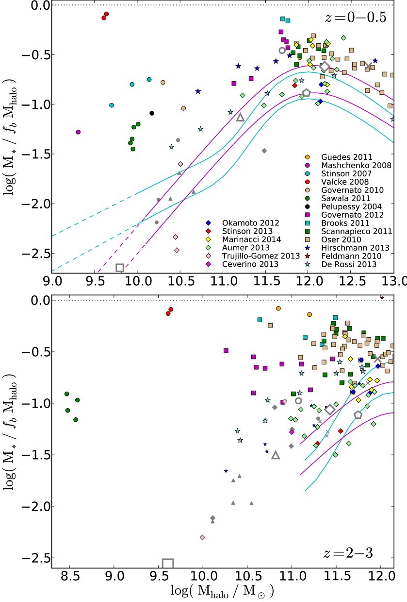
Figure 7: Comparison of the $M_{\ast}(M_{\rm halo})$ relation (as Fig. 4) predicted by other published simulations in the literature using sub-grid stellar feedback models. We compile these results (colored points), where available, at low-$z$ ($z=0-0.5$; top) and high-$z$ ($z=2-3$; bottom). We compare against the simulations presented here (gray points) with explicit feedback, and observational constraints (lines). Even sub-grid models which are “successful” near $\sim L_{\ast}$ at $z\sim 0$ over-predict $M_{\ast}(M_{\rm halo})$ by an order-of-magnitude relative to our explicit feedback simulations and observations at both low masses ($M_{\rm halo}\lesssim 10^{10}\,M_{\sun}$) and/or high redshifts ($z\gtrsim 2$). The exceptions appear to be the newest generation of sub-grid models which have been explicitly adjusted to mimic the effects of radiative feedback as well as SNe, seen in our explicit feedback models: this includes Stinson et al. (2013); Aumer et al. (2013); Ceverino et al. (2013); Trujillo-Gomez et al. (2013).

5.4 (Strong) Dependence on Feedback

The lower panel in Fig. 6 shows the effect of varying the physics of feedback: now, we see dramatic differences in $M_{\ast}(M_{\rm halo})$. Removing all feedback (every mechanism listed in § 3.3), gas cools and collapses on a dynamical time $t_{\rm dyn}$ within the disk, forming stars at a rate $\dot{M}_{\ast}\sim M_{\rm gas}/t_{\rm dyn}\sim\dot{M}_{\rm gas}$ where $\dot{M}_{\rm gas}$ is the inflow rate from the halo. Most of the baryons are turned into stars.

If we turn off SNe feedback, but retain all other forms of feedback, the results are nearly as bad: again, $M_{\ast}$ is severely overpredicted in both dwarfs and MW-mass systems. In the $\lesssim 10^{10}$ halos, with no SNe, other forms of feedback may still suppress SF significantly (so $M_{\ast}\ll f_{b}\,M_{\rm halo}$), but the masses are still much too large relative to those observed by factors of $\sim 100$. We also note that, as many previous studies have pointed out (Murray et al., 2005; McKee & Ostriker, 2007; Shetty & Ostriker, 2008; Faucher-Giguère et al., 2013), it is ultimately the momentum injected by SNe, not just the thermal energy, which regulates star formation. So as expected, if we artificially turn off the SNe momentum (coupling only thermal energy, as is common in many cosmological simulations), then in our simulations of massive ($>10^{12}\,M_{\sun}$) halos, this is nearly as bad as removing SNe entirely. In the lowest-mass dwarfs, the discrepancy is not so severe (factor $\lesssim 2$ changes in the SFH), because the mass resolution ($\sim 100\,M_{\sun}$) is such that the early expansion phases of SNe remnants (in which the thermal energy begins to be converted into momentum) are well-resolved.

If we remove radiative feedback entirely (both radiation pressure and local photo-ionization and photo-electric heating, as described in § 3.3), but retain SNe (and stellar winds), we see a nearly identical failure (to the no-SNe case) in both dwarfs and massive galaxies: while $M_{\ast}<f_{b}\,M_{\rm halo}$, far too many stars form. As we showed in Paper II, these mechanisms are critical to disrupt the dense regions of GMCs in which young stars are born, before SNe explode, and thus allowing the SNe to heat larger, lower-density volumes of gas (which can both avoid over-cooling and feel the collective effects of many SNe rather than just one), and therefore actually generate significant galactic outflows. The same result is found (on smaller scales) in much higher-resolution simulations of either single star clusters or the first stars, which directly treat the radiation-hydrodynamics with each single star as a source (e.g. Offner et al., 2009; Krumholz et al., 2011; Tasker, 2011; Wise et al., 2012).

Interestingly, in the dwarfs, if we turn off only radiation pressure, or only photo-ionization heating, the effect is much less severe: the predicted stellar mass is still significantly larger, but it is $>100$ times larger when both are removed. Radiation pressure can, to some extent, “make up for” the loss of photo-heating, and vice versa. This should actually not be surprising: the most massive GMCs in dwarf galaxies have local characteristic velocities $<10\,{\rm km\,s^{-1}}$, thus either HII heating or UV radiation pressure alone can disrupt them (though we expect, under these conditions, HII heating should dominate), and this is completely consistent with both observations of star-forming regions (e.g. Lopez et al., 2011) and numerical radiation-hydrodynamic simulations of low-density, low-velocity clouds (Harper-Clark & Murray, 2011; Sales et al., 2013). And indeed this tradeoff between photo-heating and radiation pressure in small clouds is exactly what we saw in our ultra-high resolution simulations of isolated dwarfs of the same mass (discussed extensively in Paper II; see Figs. 7, 9, and 14-19 therein).

In the massive systems, on the other hand, the radiation pressure term becomes more important than the HII heating. We see this in tests with both m12q and m12v. Even when the difference in stellar mass is not large (e.g. the m12v case), the lack of radiation pressure feedback is particularly evident in the dense, early-forming center of the galaxy, where in the runs without radiation pressure feedback an enormous central density “spike” appears, leading to a very large circular velocity of $\sim 400\,{\rm km\,s^{-1}}$ in the central regions of these systems. At these densities, HII photo-heating is dynamically insignificant.

If we disable stellar wind feedback (specifically, retaining stellar winds as a source of mass and metals, but associating no energy or momentum with that mass), and retain all other feedback, we see relatively weak effects. This is not surprising: their momentum flux is comparable to but not larger than other sources, and their energetics are much less than SNe. But they are obviously an extremely important source of mass and metals in the ISM.

5.5 Comparison to Previous Work

In Fig. 7, we compare our results (grey points) at low and high redshifts, to those from previous simulations spanning a wide range of galaxy properties and numerical methods (Pelupessy et al., 2004; Stinson et al., 2007, 2013; Mashchenko et al., 2008; Valcke et al., 2008; Governato et al., 2010, 2012; Oser et al., 2010; Feldmann et al., 2009; Brooks et al., 2011; Guedes et al., 2011; Sawala et al., 2011; Scannapieco et al., 2011; De Rossi et al., 2013; Okamoto, 2013; Kannan et al., 2013). All of these simulations include some form of sub-grid model designed to mimic the ultimate effects of stellar feedback, although the prescriptions adopted differ substantially between each. Most of these models are specifically tuned to reproduce reasonable scaling for MW-mass systems at $z\sim 0$. However, two discrepancies are immediately evident. First, nearly all the previous models predict much larger stellar masses in dwarf galaxies with $M_{\rm halo}\lesssim 10^{11.5}\,M_{\sun}$, compared to either our simulations or the observational constraints. Second, even simulations which produce excellent agreement with the observations at $z=0$ tend to predict far too much star formation at high redshift (take e.g. the simulation in Guedes et al. 2011, which produces a MW-like system with many properties consistent with observations at $z=0$, but has turned nearly all its baryons into stars at $z\gtrsim 2$).

These are similar to the discrepancies that appear when we re-run our simulations excluding radiative feedback. And indeed, nearly all of the models from the literature in Fig. 7, even given various freely adjustable parameters, are designed and motivated only to reproduce the effects of supernova feedback, which we have shown is insufficient to explain the observations.

In fact, the only sub-grid models, to our knowledge, which currently do not produce such discrepancies (and agree broadly with our simulations both at low masses and high redshifts) are the recent generation of models in Stinson et al. (2013); Aumer et al. (2013); Ceverino et al. (2013); Trujillo-Gomez et al. (2013) (for some additional results from these see Kannan et al. 2013). These new models (all of which have been developed recently) are specifically designed/tuned to mimic the effects of radiative feedback (albeit indirectly), and to reproduce via simple sub-resolution prescriptions (including turning off cooling) some of the most important effects of radiation pressure and photo-heating which were studied in our previous work (Hopkins et al., 2012d). Whether this is unique or not remains to be tested; the phase structure and other properties of outflows and the CGM in such models can be very different from those predicted here, even for the same mass-loading efficiencies (discussed further below). It will be particularly interesting to see whether other recently-developed sub-grid models such as that in Agertz et al. (2013), also incorporating the effects of radiative feedback but via very different prescriptions, will also agree well with observations at both low and high redshifts. In any case, these comparisons – and the results from this new generation of sub-grid models – highlight that some accounting for non-SNe feedback is critical.

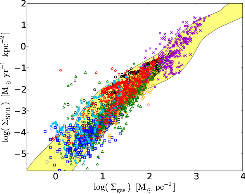
Figure 8: Kennicutt-Schmidt law, observed (Kennicutt, 1998; Bigiel et al., 2008; Genzel et al., 2010; Daddi et al., 2010, yellow shaded range) and simulated (points as Fig. 4). We emphasize that this is a prediction: the instantaneous SF efficiency per dynamical time in dense gas is $100\%$ in the simulations, but the emergent KS-law, as a consequence of feedback, has an efficiency a factor $\sim 50$ lower. As shown in Paper I and Hopkins et al. (2013d), this is insensitive, with resolved feedback models, to the small-scale star formation law, and entirely determined by stellar feedback. “No feedback” models lie a factor $\sim 50$ above the observations; “no radiation” and “no SNe” models (Fig. 6) lie a factor $\sim 10$ above observations.

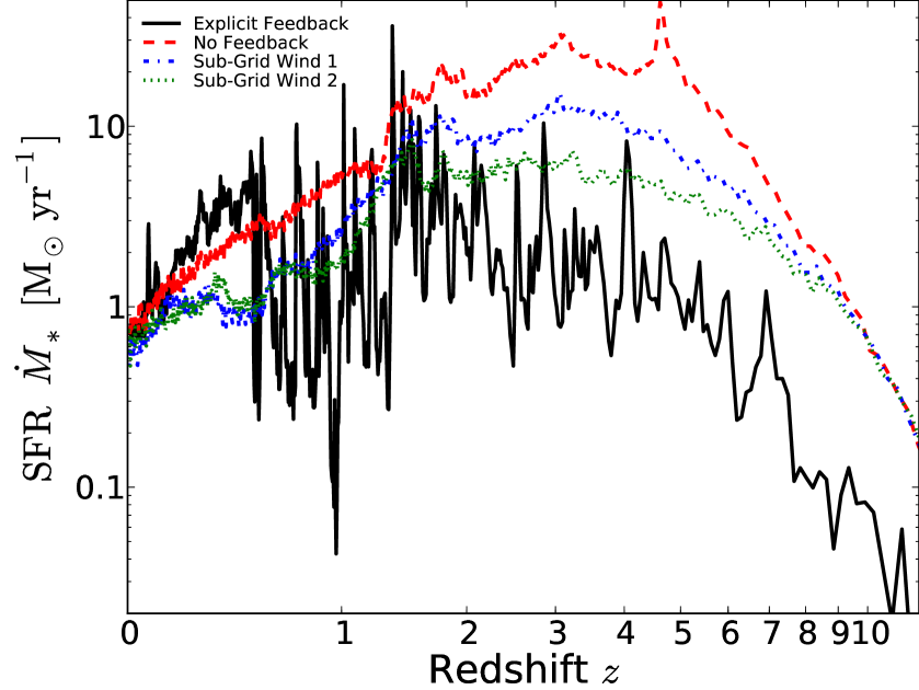
Figure 9: Example star formation history (SFH) for the m12v simulation, in our standard (explicit feedback) model compared to different sub-grid feedback treatments. We show the formation history of all stars in the simulated box at $z=0$ (smoothed in $10^{7}$ yr bins); this is not qualitatively different from the SFR versus time of the largest “main” galaxy in the box at each time. “No feedback” models force the galaxy to lie on the KS-law (SF is “slow”) but do not expel gas; gas piles up until the SFR balances the halo accretion rate, with a broad peak from $z\sim 2-6$. “Sub-grid wind” models “kick” gas at a rate proportional to the SFR; we show examples with different efficiencies and implementations. By design, model “2” produces a nearly identical $z=0$ stellar mass $M_{\ast}$ to our explicit feedback model. These sub-grid models (by construction) lower the SFR, but in both cases leave the qualitative behavior of the SFH identical. Explicit feedback models not only suppress the total $M_{\ast}$ formed, but change the shape of the SFH. SF is more “bursty” on small timescales, and the SFR is flatter in time (more biased to late times, without the broad high-$z$ peak).

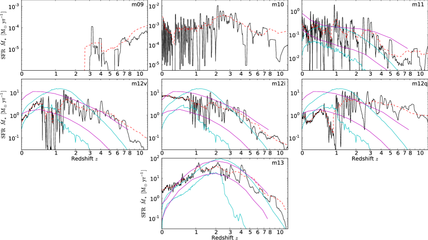
Figure 10: SFH for each “main” (largest) $z=0$ galaxy in our standard (explicit-feedback) simulations. Lines show the mean SFR averaged on timescales of $10^{8}$ yr (black solid) and $10^{9}$ yr (red dashed). With explicit feedback, SFRs are highly variable below the galaxy dynamical time. Moreover, the (averaged) SFRs tend to be flat and/or rising with time. In contrast, with no feedback, the SFH has a sharp rise and fall peaking at $z\sim 2-6$. In the least massive dwarfs (m09; $M_{\ast}<10^{6}\,M_{\sun}$ and $V_{\rm vir}(z=0)<20\,{\rm km\,s^{-1}}$), the SFR is strongly suppressed after reionization once a combination of the ionizing background and some small amount of feedback from the early star formation is able to expel most of the halo gas and prevent new cooling. We compare our ${\bf m11}$, ${\bf m12}$, and ${\bf m13}$ runs to the observationally inferred “mean” tracks (colored lines) for the main galaxies in halos of the same $z=0$ mass, from Moster et al. (2013, magenta) and Behroozi et al. (2012, cyan). In each case the lines bracket the $1\,\sigma$ range/scatter in the observed galaxy population. Our m11 and m12 runs agree very well with these constraints; however, in the most massive systems (m13), the galaxy never “quenches,” and the SFR remains high in conflict with observations below $z\sim 1$.

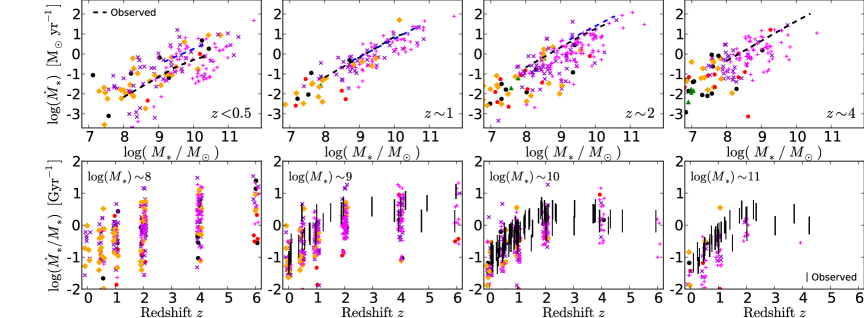
Figure 11: Top: SFR versus galaxy stellar mass at different redshifts. We compare the observed (best-fit) relations from the compilation in Behroozi et al. (2012, black dashed) and Zahid et al. (2012, blue dashed) (the systematic offset is typical of different calibrations). Allowing for the typical factor $\sim 2$ systematic observational calibration uncertainty, the agreement is good at all $z$. However, magenta $+$’s compare low-resolution ($100$ pc softening) runs of some massive halos which produce too-massive galaxies at $z=0$: there is little offset between these simulations and our fiducial models. The observed relation is simply a consequences of galaxies having relatively “flat” star formation histories. Bottom: Specific SFR of galaxies with different $M_{\ast}$, versus redshift. Observations are compiled in Behroozi et al. (2012, Table 5) and Torrey et al. (2013). The dynamic range here is smaller so the plot appears noisier, but the information is identical to that at top. SSFRs at $z\gtrsim 2$ are relatively flat, indicating rising SF histories at high-$z$.

5.6 Instantaneous Suppression of Star Formation (at Fixed Gas Densities)

We now examine galaxy star formation rates. In the previous section, we showed that the integrated SF is suppressed with feedback. But equally important is that feedback suppresses instantaneous SFRs in galaxies. This is manifest in the Kennicutt-Schmidt (KS) relation, shown in Fig. 8. We plot the simulations at all redshifts (the redshift evolution is insignificant), and compare to observations at a range of redshifts (which also find little or no evolution).

The predicted KS law agrees well with observations at all redshifts. As shown in Paper I-Paper III, this emerges naturally as a consequence of feedback, and is not put in by hand. Recall that the instantaneous SF efficiency (SF per dynamical time) in dense gas in the simulations is $100\%$; however the global SF efficiency is $\sim 2\%$. This difference arises because at $\sim 2\%$ efficiency, feedback injects sufficient momentum to offset dissipation (indeed, given the same feedback, we obtain the identical KS law independent of the details of our small-scale SF law; see Hopkins et al. 2011, 2013d).

If we instead consider simulations with weak/no feedback, the global KS relation is severely over-predicted (efficient cooling leads to global efficiencies $\sim 100\%$). In most cosmological simulations, this is offset “by hand” by simply enforcing a large-scale SF law that is sufficiently “slow” that it agrees with the observations; however we see that this is already (implicitly) a sub-grid feedback model. Including explicit feedback obviates the need for these prescriptions, meaning that the instantaneous SF properties are truly predictive, and not simply a consequence of our chosen small-scale SF law.

5.7 Global Star Formation Histories

In Fig. 9, we examine the SFH of one MW-mass galaxy. We compare this to common sub-grid models. First, a “no-feedback” model following Springel & Hernquist (2003a); this includes only a sub-grid model for the effects of stellar feedback on the ISM structure (an “effective equation of state”) which ensures, by design (via tuned parameters) that the galaxy lies on the Kennicutt-Schmidt relation and has reasonable gas densities. However, without galactic winds, gas from inflows quickly builds up and the SFR rises until $\dot{M}_{\ast}\approx\dot{M}_{\rm inflow}$, and nearly all the baryons are turned into stars. The galaxy at $z=0$ is far too massive, and most of its stars are old (formed at $z\gtrsim 2$, with the SFR peaking at $z\sim 5$). We then add a sub-grid wind model, in which gas is “kicked” out of the galaxy (forced to free-stream to ensure it escapes the disk) at a rate proportional to the SFR: here the mass-loading is equal to the SFR (“sub-grid wind 1”). This suppresses the SFR (as it is intended to do), by about a uniform factor $\sim 2$, as expected. However this still leaves a too-massive galaxy, with most of its stars formed very early. Next, we consider a stronger wind model (“sub-grid wind 2”): the mass-loading is doubled, with the free-steaming length fixed. This further suppresses the SFR – in this model the final stellar mass agrees reasonably well with our explicit-feedback simulation. However, the sub-grid model still produces a SFR which peaks at very high redshifts $z\sim 2-6$. The problem is that in all the sub-grid models – regardless of the absolute suppression of the integrated SFR or position on the Kennicutt-Schmidt relation – the shape of the galaxy SFH still closely resembles the shape of the halo inflow rate vs. time (for examples of this with other sub-grid models, see Oppenheimer & Davé, 2008; Scannapieco et al., 2011; Stinson et al., 2013; Puchwein & Springel, 2013).

These broadly peaked SF histories are disfavored by a variety of observations. They produce too-massive galaxies at high redshift, as discussed above. But they also produce galaxies with SF histories at high-$z$ that disagree with direct observational constraints (see Papovich et al., 2005; Reddy et al., 2006; Stark et al., 2009).

With our full, explicit feedback model included, we see that the shape of the SF history is qualitatively changed, and is more consistent with observations. At all times, SFRs are much more time-variable (this is discussed below). At the highest $z\gtrsim 6$, halo and stellar masses both grow efficiently (albeit with some offset). This is the “rapid assembly” phase, before/during reionization, in which feedback – while able to eject some gas from the galaxy and provide some overall suppression and variability of $\dot{M}_{\ast}$ – does not appear to dominate the gas dynamics (the central potential and mass of the halo grow on timescales comparable to the galaxy dynamical time; so $\dot{M}_{\ast}\propto\dot{M}_{\rm halo}$). But from $z\sim 2-6$, feedback acts strongly, and there appears to be a maximum, steady-state SFR which is constant or slowly increasing with time at which the galaxy is able to cycle new material into a fountain and so maintain equilibrium. This “quasi-equilibrium” SFR scales with the central potential of the galaxy (see Paper III), as traced by quantities such as the central halo density or $V_{\rm max}$ (the maximum circular velocity), not the halo mass or virial velocity. The central potential depth increases only weakly over this time as halos accrete material on their outskirts. Below $z\sim 2$, a competition ensues between slowing halo accretion rates and more highly-enriched halo gas raising cooling rates. Individual mergers also have a more dramatic effect on SF histories.

In Fig. 10, we show the SFH for each main $z=0$ galaxy in our simulations, and see that all cases with $10^{9}\lesssim M_{\rm halo}\lesssim 10^{13}\,M_{\sun}$ exhibit similar (relatively flat or slowly rising) SFHs. In the most massive halos, some decline occurs when $M_{\rm halo}\gtrsim 10^{12}\,M_{\sun}$, as the cooling time of virialized gas becomes longer relative to the dynamical time (the system transitions to “hot mode” accretion and filamentary infall is suppressed). However, we stress that the galaxies are clearly not “quenched” – every system we simulate is still very much a star-forming, blue galaxy at $z\sim 0$ (our m13 simulation would need a SFR $\ll 1\,M_{\sun}\,{\rm yr^{-1}}$ at $z=0$ to be “red and dead” by most definitions, but its SFR is $\sim 5\,M_{\sun}\,{\rm yr^{-1}}$). In very low mass halos (e.g. our m09, with $V_{\rm vir}(z=0)<20\,{\rm km\,s^{-1}}$), cooling is strongly suppressed after reionization.

5.8 Specific SFRs and the SF “Main Sequence”

Fig. 11 compares the galaxy-integrated SFRs in all our simulated systems (including non-main halos) with observations of the SFR or specific SFR (SFR$/M_{\ast}$) as a function of galaxy stellar mass, at various redshifts. The simulations agree well with the SFR “main sequence” (SFR$-M_{\ast}$ relation) observed at all $z$ (observations plotted include compilations from Erb et al. 2006; Noeske et al. 2007; Daddi et al. 2007; Elbaz et al. 2007; Stark et al. 2009 and others in Behroozi et al. 2012 (see Table 5 therein) and Zahid et al. 2012. The scatter is also similar to that observed. There may be some slight tension (the predictions being slightly high at $z=0$ and low at $z=2$), but these are well within the range of systematic uncertainties owing to different SFR calibrations (we show a couple such examples). By extension, the simulations similarly agree with the evolution in specific SFRs of galaxies as a function of mass.

Evolution in specific SFRs and SFR$-M_{\ast}$ towards higher SSFR at high-$z$ simply reflects rising gas fractions (as it must, since the simulations lie on the same KS-law in Fig. 8). The “flattening” of SSFR at high-$z$ implies SF histories of individual galaxies are rising with time (as we see directly); physically it follows from the saturation of gas fractions at large values, and rapid growth of halo mass at these times. The SFR$-M_{\ast}$ relation is, to lowest order, just $\dot{M}_{\ast}\sim M_{\ast}/t_{\rm Hubble}(z)$ – this must be trivially true in any scenario where SFRs are relatively flat and/or rising with time (typical of star-forming galaxies). For this reason we see the same relation even in our simulations without feedback, as have other simulations with different feedback prescriptions (see Kereš et al., 2009; Davé et al., 2011). And we see that even the very massive halos (which produce “too large” an $M_{\ast}$ at low redshifts) lie on the extension of the observed relation (the problem is that they continue on the relation, rather than “quenching” and moving below it, as observed at high masses).

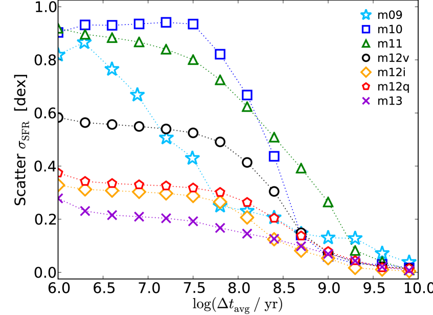
Figure 12: Variability of the SFHs shown in Fig. 10, quantified versus timescales $\Delta t_{\rm avg}$. For each “main” galaxy in each simulation, we show the logarithmic dispersion in the SFR $\sigma_{\rm SFR}$ about its mean on longer timescales, when the SFR is time-averaged over the timescale $\Delta t_{\rm avg}$. The variability rises substantially on timescales $\sim 10^{7}-10^{8}$ yr (galaxy dynamical times), owing to a combination of fountain dynamics, local structure in the galaxies, and stochastic effects from individual star forming regions. The short-timescale variability is a factor of $\sim 2-3$ in $\sim L_{\ast}$ galaxies, but rises to order-of-magnitude level in dwarfs (where individual star clusters and bursts have a more dramatic effect).

5.9 Quantifying Burstiness/Variability in SFRs

In Fig. 9, we showed that the SFRs are significantly more time-variable in models with explicit/resolved feedback as compared to sub-grid feedback models. We quantify this in Fig. 12. We measure the dispersion in the SFR smoothed over various time intervals. Unsurprisingly, the scatter is larger on small timescales. On $\gg 10^{8}\,$yr timescales, the variability is always small (SFHs are “smooth”) – this is more a function of the evolution of the halo over a Hubble time. Some such long-timescale variability is driven by mergers and global gravitational instabilities, but much of the short-timescale variability is not connected to these phenomena. Rather, on smaller timescales (comparable to the galaxy dynamical time) the dynamics of fountains, feedback, and individual giant molecular clouds and star clusters becomes important, so the scatter increases down to timescales $\sim 10^{6}\,$yr (comparable to the massive stellar evolution timescale). The short-timescale scatter is modest ($\sim 0.3\,$dex) for massive systems ($M_{\rm halo}\gtrsim 10^{12}\,M_{\sun}$), but rises in smaller halos (where even single star clusters can have large effects) to $\sim 1\,$dex at $M_{\rm halo}\lesssim 10^{10}\,M_{\sun}$.

6 Discussion & Conclusions

6.1 Key Results and Predictions

We present a series of cosmological zoom-in simulations${}^{\ref{foot:movie}}$ of galaxies with $M_{\rm halo}\sim 10^{9}-10^{13}\,M_{\sun}$ and $M_{\ast}\sim 10^{4}-10^{11}\,M_{\sun}$. At this time, several of these runs represent the highest-resolution in both mass and force resolution of any fully cosmological runs to $z=0$. But the most important improvement, compared to previous simulations, is that we for the first time include a fully explicit treatment of both the multi-phase (cold molecular through atomic, ionized, and hot diffuse) ISM and stellar feedback. Our treatment of the ISM is enabled both by our resolution and improved treatment of cooling and heating physics (e.g. molecular and metal line cooling, photo-ionization and photo-electric heating with self-shielding). Our stellar feedback model utilizes explicit time-dependent energy, momentum, mass and metal fluxes taken directly from stellar population models, without free/adjustable parameters. As such, the SFRs in our simulations, the resulting outflows, and galaxy stellar masses are not the result of tuning or “by hand” adjusting feedback efficiencies. Critically, we include not just thermal energy from SNe, but the momentum and energy associated with SNe Types Ia & II, stellar winds (young star & AGB), local photo-ionization and photo-electric heating, and radiation pressure from UV and IR photons. In addition, our formulation of SPH resolves the historical numerical problems with this method, especially important for cooling in hot halo atmospheres (see Appendix B; Hopkins 2013; Keres et al. in prep).

Our key conclusions include:

• Stellar feedback – from known sources including SNe (energy and momentum), stellar winds, radiation pressure (primarily optical/UV), and photo-heating – is both necessary and sufficient to explain the observed relation between galaxy stellar mass and halo mass, and by extension the shape of the galaxy mass function and clustering, at stellar masses $M_{\ast}\lesssim 10^{11}\,M_{\sun}$. This appears to be true at all redshifts.

• No one feedback mechanism alone is sufficient: the effects add non-linearly, and the common approximation in simulations of including only SNe feedback severely over-predicts galaxy masses (especially at low masses and/or high redshifts). The effects are even worse if the feedback momentum is ignored (if only thermal energy is considered).

• The $M_{\ast}-M_{\rm halo}$ relation evolves very weakly with redshift (because outflow efficiencies depend mostly on the central binding energy within the galaxy). At $z\gtrsim 2$, weak evolution towards higher $M_{\ast}(M_{\rm halo})$ at low masses is equivalent to a steepening faint-end slope of the galaxy luminosity function, similar to what is inferred observationally (Bouwens et al., 2007; Stark et al., 2009).

• Stellar feedback and standard cooling physics explain low galaxy stellar masses, but do not appear sufficient to explain “quenching” (late time suppression of star formation in massive halos) – none of our massive systems are “red and dead.”

• Our simulations reproduce the observed Kennicutt-Schmidt relation. This is despite the fact that we assume a small-scale SF efficiency of $100\%$ in self-gravitating dense gas. As such, the KS law and instantaneous SFRs are truly predicted, not simply a consequence of our sub-grid SF law. The low star formation efficiency we find is a consequence of stellar feedback, not the microphysics of how stars form in dense gas. Absent feedback, efficient cooling leads to a global SF efficiency of $\sim 100\%$ per dynamical time. With feedback – from the same mechanisms that produce large-scale outflows and regulate galaxy formation – the SF efficiency self-regulates at $\sim 2\%$, the level where feedback injects sufficient momentum to offset dissipation.

• Realistic feedback changes the shape of galaxy star formation histories. In particular, feedback from stellar radiation (both photo-heating and radiation pressure) is critical for disrupting dense, cold gas, and so is especially important for suppressing star formation in high redshift galaxies. This leads to much flatter, or gently rising, star formation histories in sub-$L_{\ast}$ galaxies. Most previous sub-grid models give qualitatively different results, in conflict with observations.

• The observed star formation “main sequence” and specific SFRs emerge naturally from the shape of the galaxies’ star formation histories (from $M_{\ast}\sim 10^{8}-10^{11}$ and $z\sim 0-6$). This includes “flat” SSFR evolution at $z\sim 2-6$. However these are relatively insensitive to feedback, since any broadly flat or rising SF history predicts $M_{\ast}(z)\sim t_{\rm Hubble}(z)\,\langle\dot{M}_{\ast}(z)\rangle$, consistent with the observations.

• Dwarf galaxies exhibit much more “bursty” SF histories, with large variability in their SFRs on short timescales ($\sim 1\,$dex scatter on $\lesssim 10^{7}\,$yr timescales). This is because star formation and star cluster formation, and their associated feedback, are stochastic. The variability is not driven by mergers or global gravitational instabilities. Massive ($\sim L_{\ast}$) galaxies are much less variable ($\sim 0.3\,$dex scatter in SFRs). This may translate into significantly larger scatter in $M_{\ast}(M_{\rm halo})$ at dwarf masses compared to $\sim L_{\ast}$ galaxies.

6.2 Numerical Methods

We see relatively weak dependence on simulation resolution, which is perhaps surprising given the small-scale structure present in the ISM. However, in Papers I-III & Appendix C, we presented extensive resolution studies of isolated disk galaxies simulated using the same prescriptions but numerical resolution varied from values comparable to those here, to order-of-magnitude superior mass and spatial resolution. We showed that the galaxy-averaged SFR is one of the very first quantities to converge, and is consistent to within factor $\sim 2$ even for relatively poor resolution: this is because it traces the integral effect of feedback balancing turbulent dissipation. That said, we do see qualitative changes in behavior if the resolution falls below that needed to meaningfully resolve ISM phase structure, at which point “self-regulation” by feedback loses meaning. As a rule of thumb, the simulations must at least resolve the Toomre/Jeans length and mass (the size of the largest GMCs) in each star-forming disk, and the results are especially numerically stable if the mass resolution can be ideally pushed to $<10^{4}\,M_{\sun}$. Even in this regime, quantities such as the phase structure of dense gas and outflows are much more sensitive to resolution, and will be discussed in more detail in future work.

Given the same feedback model, we also see little difference in the stellar mass buildup between our standard simulations, run with a numerical algorithm designed and shown to eliminate essentially all major differences between grid (Eulerian) and smoothed-particle (Lagrangian) hydrodynamics methods, and an older version of SPH that exhibits large differences in test problems. Thus we expect little or no difference between the results here and those from adaptive-grid or moving-mesh codes, if the same feedback and ISM physics could be included. This owes to two key points: first, the differences between numerical methods in this respect, even where significant, are generally much smaller than the orders-of-magnitude differences owing to the inclusion or exclusion of the relevant physics. The stellar mass content of galaxies is set by the total amount of feedback injected, and so it is unsurprising that the time-averaged star formation rate is insensitive to changes in the detailed phase structure of the gas around galaxies. Second, the numerical differences primarily affect mixing instabilities in multi-phase, sub-sonic, pressure-dominated gas. As such, many comparison studies have shown that while the numerical differences can be important for details of the structure of hot halos in massive galaxies, they are generally unimportant inside cold star-forming gas, or in sub-$L_{\ast}$ halos, where the flows of interest tend to be highly super-sonic and gravity-dominated (see e.g. Kitsionas et al., 2009; Price & Federrath, 2010; Bauer & Springel, 2012; Sijacki et al., 2012). As one considers more detailed galactic properties, we expect the differences between numerical methods to manifest as discrepancies in the cooling properties, phase structure, or distribution of heavy elements in the CGM, and to impact the way in which both inflowing cool gas and feedback-driven outflows interact with gas in galactic halos. For these reasons, an accurate numerical scheme is critical if one hopes to study the detailed structure of both gas in and around galaxies with realistic feedback. A much more extensive comparison of numerical methods is presented in a companion paper (Kereš et al., 2014).

6.3 Future Work

This is a first exploration of cosmological simulations with explicit stellar feedback models, and many open questions remain. We have studied the effects of realistic stellar feedback on galaxy star formation histories and stellar masses; however, a complete understanding of this self-regulation requires a much more detailed examination of the dynamics of galactic outflows. In companion papers, we will study how outflows are generated, and how these interact with the circum-galactic and inter-galactic medium. It will be particularly important to build new observational diagnostics and explore whether or not different feedback mechanisms lead to different observable properties in the ISM, CGM, and IGM (Faucher-Giguere et al., 2014). Complementary questions regarding the morphology of galaxies – how the sizes, bulge-to-disk ratios, kinematics, and other properties of the simulated systems here depend on different feedback mechanisms – will be developed as well. The resolution and explicit treatment of the ISM in these simulations make possible many additional studies.

Going forward, it will also be important to examine the role of additional physics. Some other physics is probably needed to explain the “quenching” of star formation in massive systems ($M_{\rm halo}\gg 10^{12}\,M_{\sun}$). AGN feedback is a plausible candidate, which we have studied in previous work using idealized sub-grid models for the ISM. But the consequences could easily be completely different in a resolved multi-phase medium. Other physics such as magnetic fields, anisotropic conduction, and cosmic rays may be important as well, and their consequences are just beginning to be explored (e.g. Jubelgas et al., 2008; Hanasz et al., 2013; Salem & Bryan, 2013).

Appendix A Baryonic Physics: Details of the Algorithmic Implementation

A.1 Cooling

Gas cooling is solved implicitly each timestep (using the iterative algorithm from GADGET-3). Heating/cooling rates are computed including free-free, photo-ionization/recombination, Compton, photo-electric, metal-line, molecular, and fine-structure processes. We follow $11$ separately-tracked species (H, He, C, N, O, Ne, Mg, Si, S, Ca, and Fe, each with its own yield tables associated directly with the different mass return mechanisms below; see Wiersma et al. 2009b). The appropriate ionization states and cooling rates are tabulated from a compilation of CLOUDY runs, including the effect of a uniform but redshift-dependent photo-ionizing background computed in Faucher-Giguère et al. (2009), together with local sources of photo-ionizing and photo-electric heating (described below with the relevant feedback mechanisms). Self-shielding is accounted for with a local Sobolev/Jeans-length approximation (integrating the local density at a given particle out to a Jeans length to determine a surface density $\Sigma$, then attenuating the background seen at that point by $\exp{(-\kappa_{\nu}\,\Sigma)}$). Confirmation of the accuracy of this approximation in radiative transfer experiments can be found in Faucher-Giguère et al. (2010) and Rahmati et al. (2013). With this accounting, metal-line cooling follows the rate tables from Wiersma et al. (2009a), free-free rates follow Katz et al. (1996), and photo-electric rates follow Wolfire et al. (1995). Compton heating/cooling is included both from the CMB and local sources, accounting as in Faucher-Giguere & Quataert (2012) for possible two-temperature plasma effects at very high temperatures by limiting the Compton rates by the Coulomb energy exchange rates (though in practice this is only relevant at much higher temperatures than are seen in these simulations). Fine-structure and molecular cooling at low temperatures ($T<10^{5}\,$K) is tracked using an interpolation table for a compilation of CLOUDY runs as a function of the density, temperature, metallicity, and local ionizing background, as in Robertson & Kravtsov (2008). A temperature floor is included at the maximum of either $10\,$K or the CMB temperature at the given redshift.

A.2 Star Formation

Star formation occurs probabilistically. At each timestep ${\rm d}t$, a gas particle has a probability of turning into a star particle $p=1-\exp{(-\dot{m}_{\ast}^{i}\,{\rm d}t/m^{i}_{\rm gas})}$, where $\dot{m}_{\ast}^{i}$ is the SFR integrated over the particle, and $m_{\rm gas}^{i}$ is the particle gas mass. The SFR is non-zero only for particles with density above $n>n_{\rm crit}$ (generally $n_{\rm crit}=100\,{\rm cm^{-3}}$), which are also locally self-gravitating using the criteria developed in Hopkins et al. (2013d) ($\alpha\equiv\delta v^{2}\,\delta r/G\,m_{\rm gas}(<\delta r)\approx\beta\,(|\nabla\times{\bf v}|^{2}+|\nabla\cdot{\bf v}|^{2})/G\,\rho<1$, with $\beta\approx 0.25$), and which have a non-zero molecular fraction $f_{\rm mol}>0$. The molecular fraction is determined following Krumholz & Gnedin (2011), using the local Sobolev approximation and metallicity to estimate the integrated column to dissociating radiation ($\tau\approx\kappa\,\langle\Sigma\rangle$ with $\langle\Sigma\rangle=\rho\,[h_{\rm sml}+(\nabla\,\ln{\rho})^{-1}]$ and $\kappa=\kappa_{\rm gas}+\kappa_{\rm dust,\,MW}(Z/Z_{\odot})$). The SFR per unit volume for gas that meets all of these criteria is then $100\%$ per free-fall time, $\dot{\rho}_{\ast}=\rho_{\rm mol}/t_{\rm ff}=f_{\rm mol}\,\rho_{\rm gas}/t_{\rm ff}$. When a gas particle becomes a star particle, the star particle inherits the metallicity of each followed species from its parent, and the conversion/formation time of the particle is used to determine its age in subsequent timesteps. The star particles also inherit their mass and gravitational softening from their parent gas particles, so that they are not over or under-resolved relative to the medium from which they form.

A.3 Stellar Feedback

The stellar feedback algorithms follow those developed in Paper I-Paper II, with some modifications necessary for cosmological simulations.

Radiation Pressure: Gas surrounding stars (see below) receives a direct momentum flux $\dot{P}_{\rm rad}\approx(1-\exp{(-\tau_{\rm UV/optical})})\,(1+\tau_{\rm IR})\,L_{\rm incident}/c$ where $1+\tau_{\rm IR}=1+\Sigma_{\rm gas}\,\kappa_{\rm IR}$ accounts for the absorption of the initial UV/optical flux and multiple scatterings of the re-emitted IR flux if the region between star and gas particle is optically thick in the IR (assuming the opacities scale linearly with gas metallicity). At each timestep we evaluate the optical depth in a smoothing kernel around the star particle (whose pre-absorption stellar spectrum $L_{\nu}$ is tabulated as a function of age and metallicity). The UV/optical absorption ($\tau_{\rm UV/optical}=\int\,\kappa\,\rho\,{\rm d}\ell$) is estimated via the Sobolev approximation (as above) in multiple frequency bins (see Paper II for details). The absorbed fraction of $L$ is then distributed within the SPH smoothing kernel according to each particles’ relative contribution to the optical depth. This absorbed luminosity is assumed to re-radiate isotropically in the IR (and while it can be re-absorbed, it is again re-radiated in the IR), so for an (assumed) gray-body opacity it imparts an acceleration $a_{\rm IR}=\kappa_{\rm IR}\,F_{\rm IR}/c$ to all gas in the kernel.

Photons which are not absorbed in the UV/optical, and the re-emitted IR flux, define an effective “emergent spectrum” for each kernel. This is propagated to large distances in the gravity tree, where it is used to calculate the local incident flux on all gas particles from stars outside the smoothing kernel; the same frequency-dependent opacities are used to calculate the local absorption and momentum flux ($\dot{P}=L_{\rm abs}/c$). The momentum flux is imparted in every timestep along the direction determined by the flux-limited diffusion approximation (along the local optical depth gradient).

Photo-Ionization and Photo-Electric Heating: Here the algorithm is identical to that in Paper II. We first tabulate the rate of production of ionizing photons for each star particle (as a function of age and metallicity); moving radially outwards from the star, we then ionize each neutral gas particle until the photon budget is exhausted (using the gas density, metallicity, and ionization state to determine the necessary photon number). Note that – unlike the purely local Stromgren sphere approximation sometimes used in the literature – this accounts for whether each particle is already ionized, and (if so) allows the ionized region to continue to expand (thus accounting for large coherent/overlapping HII regions). In the cooling routine, ionized gas is flagged as having a sufficiently strong local ionization field to keep it fully ionized for the duration of the timestep; this local ionizing field information together with the escaped UV flux defined above is also used to determine the photo-electric heating rates in the cooling routine.

Supernovae and Stellar Winds: The SNe Type-I and Type-II rates are tabulated from Mannucci et al. (2006) and STARBURST99, respectively, as a function of age and metallicity for all star particles; this determines a probability per unit time ${\rm d}p=({\rm d}N_{\rm SNe}/{\rm d}M_{\ast}\,{\rm d}t)\,m_{\ast,\,i}\,{\rm d}t$ which we use to determine whether a SNe occurs in a given particle each timestep drawing from a Poisson distribution. If so, the appropriate ejecta mass, metal yields (for all followed species), energy, and momentum are tabulated and directed radially from the star, and we assume the ejecta shocks within the gas in the smoothing kernel $h_{\rm sml}$ (appropriately weighted) around the star.

However, coupling this appropriately requires knowing whether the shock is energy or momentum conserving up to the scales we resolve. To estimate this, consider the cooling radii calculated in high-resolution simulations of individual blastwaves: $R_{\rm cool}\approx 28\,{\rm pc}\,E_{51}^{0.29}\,\langle n_{\rm cgs}\rangle^{-0.43}\,(Z/Z_{\odot}+0.01)^{-0.18}$ (where $E_{51}\approx 1$ is the ejecta energy in units of $10^{51}\,{\rm erg\,s^{-1}}$; $\langle n_{\rm cgs}\rangle$ is the local density in ${\rm cm^{-3}}$; and $Z$ is the local gas metallicity; see Cioffi et al. 1988). When $h_{\rm sml}\ll R_{\rm cool}$, the full ejecta (shocked) kinetic energy is coupled as thermal energy (with the ejecta momentum included as a momentum flux, and the ejecta mass and metals as mass/metal fluxes into the gas). Otherwise, at coupling, a fraction of the initial ejecta energy is instead converted from energy into momentum as would occur within the un-resolved cooling radius so the coupled momentum is ${\bf p}={\bf p}_{\rm ej}\,\sqrt{[M_{\rm ejecta}+M_{\rm enc}(<R_{\rm cool})]/M_{\rm ejecta}}$, and an additional fraction of the shocked thermal energy is cooled away before being allowed to artificially do any work (according to $E_{\rm thermal,\,shocked}\propto(R/R_{\rm cool})^{-6.5}$; see Thornton et al. 1998). We stress that this is very different from assuming the SNe energy goes directly into a wind, or from turning off cooling in the gas. We are simply accounting for the possibility of an unresolved Sedov-Taylor phase and depositing the appropriate momentum, not just thermal energy, in the ambient medium in that case.

As noted in the text, at high redshifts, the progenitors of massive galaxies ($\gtrsim 10^{12}\,M_{\sun}$) are not as well mass-resolved, given our particle masses of $\sim 10^{4}\,M_{\sun}$. At $z\sim 6$, the progenitor of a $z=0$, $10^{12}\,M_{\sun}$ halo has $M_{\rm halo}\sim 10^{10}\,M_{\sun}$ and so should have $M_{\ast}\sim 10^{7}\,M_{\sun}$, just $\sim 1000$ particles. As such, the details of how momentum from SNe is coupled into a kernel of $\sim 100$ particles can have significant effects on the entire baryonic galaxy. For example, we see significant changes to the SFR at $z\gtrsim 4$ if we “cap” the momentum input at a modest value ${\bf p}\approx 20\,{\bf p}_{\rm ej}$. However at lower redshifts (or in simulations with better mass resolution, such as our dwarf galaxies) this has no systematic effect (as shown in Fig. 6, where we substantially vary both the power-law scaling of the SNe momentum above and the coupling weights within the SPH kernel, and see only small effects on the final stellar mass). Because of the scaling of remnant momentum with entrained mass, the key criterion is whether the mass resolution of the simulation is $\gg M_{\rm ejecta}$. In practice we find that this explicit accounting for the SNe remnant momentum has little effect when particle masses are $\lesssim 1000\,M_{\sun}$. We have also re-run all our simulations using the alternative cooling radius estimate from Chevalier (1974): $R_{\rm cool}\approx 58\,{\rm pc}\,E_{51}^{0.32}\,\langle n_{\rm cgs}\rangle^{-0.16}\,(P_{\rm gas}/10^{-12}\,{\rm dyn\,cm^{-2}})^{-0.2}$. This makes little difference to the stellar masses and star formation histories here (there is no significant difference in their consistency with observations); the primary effect is from dropping the metallicity dependence (leading to slightly less efficient feedback in low-metallicity, poorly-resolved regions).

Stellar winds are algorithmically nearly identical to SNe, except they occur continuously. We tabulate the wind mass, metal, energy, and momentum fluxes (as a function of stellar age and metallicity), and inject these into the neighboring gas identically to the SNe.

In both cases, we include the relative gas-star particle velocities added to the wind/ejecta velocity centered on the star in calculating the initial ejecta momentum and energy fluxes, but this has very little effect in star-forming systems (since massive star winds and SNe ejecta are fast compared to the relative velocity of stars). This can, however, be significant in old stellar populations when AGB ejecta (with wind launching velocities $\lesssim 10\,{\rm km\,s^{-1}}$) dominate the mass loss.

Appendix B Simulation Numerical Details

As noted in the text, these runs adopt the P-SPH formulation of TreeSPH in GIZMO, which features many improvements to SPH and has been tested in a wide range of problems (listed in the main text). We describe the most important differences between our numerical method and previous widely-used algorithms below.

B.1 SPH Formulation

The simulations use the Lagrangian “pressure-entropy” formulation of the SPH equations developed in Hopkins (2013). This formulation derives the SPH equations exactly from the particle Lagrangian and manifestly conserves momentum, energy, angular momentum, and entropy (in the absence of sources/sinks), and also eliminates the artificial “surface tension” error term which appears at contact discontinuities in previous (“density-energy” or “density-entropy”) formulations of SPH (see also Saitoh & Makino, 2013). The pressure-entropy formulation dramatically improves the behavior of fluid mixing instabilities (e.g. the Kelvin-Helmholtz and Rayleigh-Taylor instabilities), and eliminates most of the known differences between the results of grid and SPH methods for the problems of interest here (for discussion of these in historical SPH implementations, see Agertz et al., 2007; Price & Federrath, 2010; Bauer & Springel, 2012). For extensive numerical tests, see Hopkins (2013).

B.2 Artificial Viscosity & Entropy

In SPH, the algorithm is inherently inviscid and some artificial viscosity is necessary to capture shocks. We adopt the “inviscid SPH” viscosity prescription with higher-order switches from Cullen & Dehnen (2010). This allows for excellent shock-capturing, while reducing the viscosity to identically zero away from shocks. A wide range of tests of this algorithm are presented therein. This viscosity treatment allows accurate treatment of sub-sonic turbulence down to Mach numbers $\lesssim 0.1$ while simultaneously accurately capturing shocks with Mach numbers over $\sim 10^{4}$.

Similarly, SPH is inherently dissipationless, so a mechanism is also needed to generate mixing entropy in shocks. We implement this following Price (2008), using the same higher-order dissipation switch from Cullen & Dehnen (2010): this ensures that entropy exchange only occurs in crossing, sub resolution-scale flows with discontinuous entropies (i.e. prevents artificially multi-valued entropies). For comparison, “traditional” GADGET (Springel & Hernquist, 2002) adopts a constant artificial viscosity following Gingold & Monaghan (1983) with a Balsara (1989) switch, and no entropy diffusion. This is far more dissipative, and smears out structure in sub-sonic turbulence as well as producing large (artificial) shear viscosities, which can lead to significant angular momentum transfer and eliminate structure in sub-sonic turbulence.

We have also implemented the identical artificial viscosity and dissipation switches, and higher-order spatial gradient estimators, from Read & Hayfield (2012). We have re-run a couple of our simulations using these methods, making our hydrodynamic solver essentially identical to that in SPHS. This produces only small differences, with higher mean artificial viscosity in turbulent regions, and lower in “smooth” spatially extended shocks (e.g. large-scale structure; for a comparison showing this method gives similar results to grid codes for cosmological accretion/halo gas, see Power et al., 2013).

B.3 Thermodynamic Evolution & Timestep Criteria

We employ a standard adaptive timestep algorithm and limiter. As shown in Saitoh & Makino (2009) and Durier & Dalla Vecchia (2012), in problems with high Mach number flows, adaptive timesteps (without a limiter) can lead to errors if particles with long timesteps interact suddenly mid-timestep with those on much shorter timesteps. Fortunately this is easily remedied by our timestep limiter, identical to that in Durier & Dalla Vecchia (2012). At all times, any active particle informs its neighbors of its timesteps and none are allowed to have a timestep $>4$ times that of a neighbor. Whenever a timestep is shortened (or energy is injected in feedback) particles are forced to return to the timestep calculation. The limiter is not included in the “traditional” (Springel & Hernquist, 2002) GADGET.

We have confirmed the importance of this limiter in our simulations: if it is absent, a small number of particles in explosive blastwaves generate large energy conservation errors which can artificially over-heat under-dense regions of the IGM. Provided the switch is included it makes no difference if we restrict the timestep ratio between neighbors to $2,\,4,\,6$ or $8$.

B.4 Smoothing Kernel

We adopt a quintic (fifth-order) spline kernel, with neighbor number designed to optimally resolve sound waves down to a wavelength $\approx h$, the “core radius” of the kernel. The kernel size is adaptive (following the approximate “fixed mass in kernel” prescription in Springel & Hernquist 2002), enclosing $\sim 64$ neighbors. This choice is the “optimal” spline kernel suggested by a wide range of tests in Hongbin & Xin (2005), Dehnen & Aly (2012), and Hopkins (2013). However we have also experimented with the Wendland kernels in Dehnen & Aly (2012) and triangular kernels in Read et al. (2010) and see no significant improvements up to neighbor numbers $\sim 500$. For comparison, the traditional GADGET kernel is a cubic spline. This becomes unstable outside the range $\sim 30-50$ neighbors; within this range, the “effective resolution” of the kernel is identical to that adopted here, but kernel errors are larger by nearly an order of magnitude.

B.5 Gravity

The gravity solver follows the GADGET-3 hybrid tree-particle mesh (Tree-PM) method. However, we have modified this to allow for adaptive gravitational softenings and to more accurately symmetrize the force between interacting particles with different softening, following the fully Lagrangian method in Price & Monaghan (2007); this manifestly maintains conservation of energy, momentum, and angular momentum. In “traditional” GADGET, softenings are not adaptive, and pairwise interactions are simply smoothed by the larger of the two particle softenings.

We have also modified the softening kernel as described therein (see also Barnes, 2012) to represent the exact solution for the potential of the SPH smoothing kernel. With this change, the softening no longer represents non-Newtonian gravity; rather, the gravitational force is exactly Newtonian on small scales, but for particles which are not point masses but represent the extended mass distribution represented by the SPH kernel (matching the assumption made in the hydrodynamic equations).

We have also tested most of our “standard” simulations with fixed gravitational softening lengths for the baryons equal to the minimum values in Table 1, and for the high-resolution dark-matter particles equal to $(20,\,20,\,50,\,150,\,150,\,150,\,200)\,{\rm pc}$ for runs (m09, m10, m11, m12v, m12q, m12i, m13). The latter corresponds very roughly to the dark matter softening kernel extent matching the mean inter-particle spacing at $\sim R_{\rm vir}/4$. Of course, with fixed softenings matched to Table 1, the baryons will be under-softened (i.e. can undergo hard scatterings) when they are very diffuse (in e.g. the inter-galactic medium), but we are most concerned with accuracy in the dense regions in the actual galaxy we are simulating, where smaller softenings are more accurate. In any case this produces only small differences ($\lesssim 10\%$ in stellar mass at $z=0$). Re-running a couple simulations with fixed softenings but dark matter softenings equal to the smaller minimum values in Table 1 (chosen to match the kernel extent and inter-particle spacing at $\sim 10$ kpc in each simulation) similarly produces little effect. We have also re-run several of our simulations using identical softenings for both the baryonic and dark matter particles (with that softening taken to be about the geometric mean of the two values in Table 1). The differences are again small, comparable to our slightly lower-resolution runs; if we compare to a run with different baryon/dark matter softenings but the baryonic softening matched to these new runs, the differences are almost completely eliminated. There is almost no difference, between the models above, in the predicted central dark matter profiles (Oñorbe et al., in prep).

B.6 Domain Decomposition & Parallelization

The simulation architecture has been heavily optimized from previous versions of the code. Gravity is still solved with a TreePM algorithm, with nested PM grids solving the large-scale forces while the tree is used for small-scale interactions. But the tree walk, domain decomposition, feedback routines, and SPH density and hydrodynamic force calculation have all been optimized substantially relative to the GADGET-3 implementation (increasing the memory requirement by a factor of $\sim 3-5$, but decreasing run-times and load-imbalances by a factor $\sim 5$). The code has also been optimized for hybrid OpenMP+MPI application, allowing near-ideal strong scaling to $\approx 256$ cores and modest gains to $512$ cores in pure-MPI mode, and positive strong scaling (a decrease in wall-clock time for runs of fixed size, albeit less than ideal) to $>1000$ cores in hybrid mode for runs presented in this work.

Appendix C Testing in Idealized, High-Resolution Galaxy Simulations

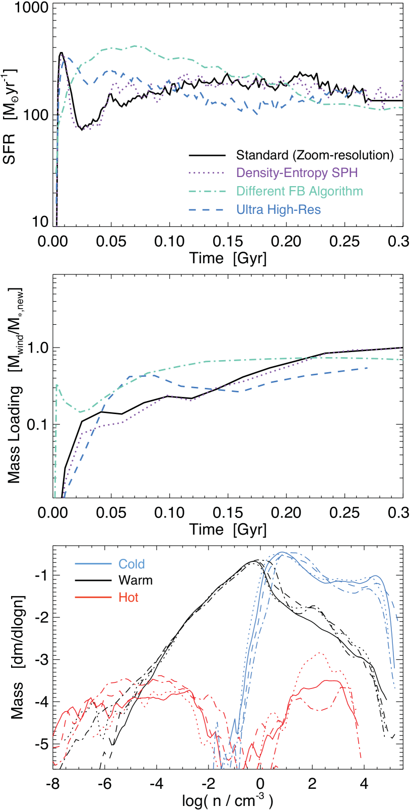
Figure 13: Tests of our methodology in idealized simulations of a single, isolated (non-cosmological), gas-rich massive disk galaxy. Top: SFR versus time. Middle: Wind mass-loading (unbound mass $M_{\rm wind}$ versus total mass in new stars formed since the beginning of the simulation). Bottom: Distribution of gas densities at fixed time $\approx 200\,$Myr after the beginning of the simulation. We separate different phases by temperature: cold gas ($T<5000\,$K), warm gas ($5000\,$K$<T<10^{5}\,$K) and hot gas ($T>10^{5}$ K; the bimodal distribution reflects low-density, high volume-filling factor material which has escaped the disk, and hot bubbles actively heated by SNe within it). In each, we compare four runs with identical initial conditions (different linestyles, as labeled). (1) A model run with our standard numerical method, at resolution about equal to our zoom-in simulations of massive galaxies. (2) A run using the density-entropy form of SPH, with our improvements to the numerical method from § B removed. (3) A run using the exact same feedback algorithms used in Paper II-Paper III, without the optimizations for cosmological runs described in § A. (4) A run at the ultra-high resolution from those papers, with much better spatial and mass resolution than can be achieved in cosmological runs. We see very little difference between the runs, suggesting both that our results are stable with respect to resolution and that the changes to the code and resolution for cosmological simulations do not fundamentally alter our conclusions from the previous work.

In a series of papers (Paper I-Paper III), we have extensively studied and tested the feedback models used here in even higher-resolution simulations of idealized (non-cosmological) individual model galaxies. Our dwarf galaxy simulations here are run at essentially the same resolution as the “ultra-high resolution” dwarf galaxy models in these earlier papers, so we can safely apply the same feedback models. However, as noted in the text, in the simulations of massive halos ($\gtrsim 10^{12}$) here, we are forced to lower resolution (comparable to the “high-resolution,” but not “ultra-high resolution” simulations therein); it is therefore important to check the results of the isolated galaxy simulations at lower resolution as well.

To this end, we have re-run the “HiZ” simulation from Paper I-Paper III, with the identical code used for the cosmological simulations here. This was the most massive system considered therein, a disk with properties typical of star-forming galaxies at $z\sim 2-4$. The halo, stellar bulge, stellar disk, and gas disk have masses $M_{\rm halo}=1.4\times 10^{12}\,M_{\sun}$, $M_{\rm bulge}=0.7\times 10^{10}\,M_{\sun}$, $M_{\rm\ast,\,disk}=3\times 10^{10}\,M_{\sun}$, and $M_{\rm gas}=7\times 10^{10}\,M_{\sun}$, with scale-lengths for the gas and stellar disk $h_{\rm\ast,\,disk}=1.6\,{\rm kpc}$ and $h_{\rm gas}=3.2\,{\rm kpc}$. We re-run this at two resolutions: first, the “ultra-high resolution” level used in our earlier papers, with force softening $\approx 3$ pc, and particle mass $\approx 800\,h^{-1}\,M_{\sun}$. Second, at resolution about equal to our massive cosmological simulations, force softening $\approx 10\,$pc and particle mass $\approx 5\times 10^{4}\,M_{\sun}$.

The results are shown in Fig. 13. We specifically compare the SFR and wind mass-loading versus time, and the phase distribution of the gas at a time $t\approx 200\,$Myr when the galaxy has reached a quasi-steady state. The mass loading is defined as the instantaneous ratio of total wind mass (defined as the gas mass which has positive Bernoulli parameter – i.e. would escape in the absence of additional forces or cooling – with outward radial velocity $>100\,{\rm km\,s^{-1}}$) to total stellar mass formed since the beginning of the simulation. In all cases, the steady-state SFR, wind mass-loading, and gas phase distribution are similar (to within a factor $<2$). The largest differences appear at very early times, and are generally artifacts of the initial conditions (in which the disk is supported by thermal pressure, before a turbulent cascade is established); these should not appear in our cosmological simulations.

We have also re-run this second “cosmological resolution” simulation with the identical feedback implementation used in Paper II (as opposed to the updated algorithms described above), to examine whether the improvements to the code would substantially change our previous results. We see very little difference. Since the total energy and momentum inputs are fixed to the same levels by the initial mass function, and no fundamentally new source of feedback has been introduced, this is a reassuring indication that the results are not especially sensitive to the purely numerical details of the algorithmic implementation of feedback.

As a final comparison, we re-run the simulation using the identical feedback implementation, but adopting the “density-entropy” form of SPH, with a constant artificial viscosity, no entropy diffusion, a cubic spline kernel, and constant (non-adaptive) gravitational softenings. This is the form of SPH which exhibits the largest and most severe differences from grid codes in test problems (especially involving fluid mixing). But consistent with our comparison in Fig. 6, we see almost no difference between this simulation and our new SPH run. This is consistent also with our comparison in Hopkins (2013), where we perform a similar comparison with a model dwarf (SMC-mass) galaxy. At those masses we saw almost no difference in SFR, and $\sim 50\%$ differences in the wind mass-loading owing to purely numerical effects, mostly the effect of fluid mixing instabilities altering the cooling time of hot SNe “bubbles.” In the HiZ galaxy model considered here, these differences are further minimized because the hot gas is not the dominant driver of outflows.

References

- Agertz et al. (2013) Agertz, O., Kravtsov, A. V., Leitner, S. N., & Gnedin, N. Y. 2013, ApJ, 770, 25
- Agertz et al. (2007) Agertz, O., et al. 2007, MNRAS, 380, 963
- Aguirre et al. (2001) Aguirre, A., Hernquist, L., Schaye, J., Weinberg, D. H., Katz, N., & Gardner, J. 2001, ApJ, 560, 599
- Aumer et al. (2013) Aumer, M., White, S. D. M., Naab, T., & Scannapieco, C. 2013, MNRAS, 434, 3142
- Balsara (1989) Balsara, D. S. 1989, Ph.D. thesis, Univ. Illinois at Urbana-Champaign
- Barnes (2012) Barnes, J. E. 2012, MNRAS, 425, 1104
- Bate (2012) Bate, M. R. 2012, MNRAS, 419, 3115
- Bauer & Springel (2012) Bauer, A., & Springel, V. 2012, MNRAS, 423, 3102
- Behroozi et al. (2012) Behroozi, P. S., Wechsler, R. H., & Conroy, C. 2012, ApJ, in press, arXiv:1207.6105
- Bigiel et al. (2008) Bigiel, F., Leroy, A., Walter, F., Brinks, E., de Blok, W. J. G., Madore, B., & Thornley, M. D. 2008, AJ, 136, 2846
- Blitz & Rosolowsky (2005) Blitz, L., & Rosolowsky, E. 2005, in Astrophysics and Space Science Library, Vol. 327, The Initial Mass Function 50 Years Later; Springer, Dordrecht, ed. E. Corbelli, F. Palla, & H. Zinnecker, 287
- Bournaud et al. (2010) Bournaud, F., Elmegreen, B. G., Teyssier, R., Block, D. L., & Puerari, I. 2010, MNRAS, 409, 1088
- Bournaud et al. (2011) Bournaud, F., et al. 2011, ApJ, 730, 4
- Bouwens et al. (2007) Bouwens, R. J., Illingworth, G. D., Franx, M., & Ford, H. 2007, ApJ, 670, 928
- Brook et al. (2011) Brook, C. B., et al. 2011, MNRAS, 415, 1051
- Brooks et al. (2011) Brooks, A. M., Solomon, A. R., Governato, F., McCleary, J., MacArthur, L. A., Brook, C. B. A., Jonsson, P., Quinn, T. R., & Wadsley, J. 2011, ApJ, 728, 51
- Ceverino et al. (2013) Ceverino, D., Klypin, A., Klimek, E., Trujillo-Gomez, S., Churchill, C. W., Primack, J., & Dekel, A. 2013, MNRAS, in press, arXiv:1307.0943
- Chen et al. (2010) Chen, Y.-M., Tremonti, C. A., Heckman, T. M., Kauffmann, G., Weiner, B. J., Brinchmann, J., & Wang, J. 2010, AJ, 140, 445
- Chevalier (1974) Chevalier, R. A. 1974, ApJ, 188, 501
- Cioffi et al. (1988) Cioffi, D. F., McKee, C. F., & Bertschinger, E. 1988, ApJ, 334, 252
- Coil et al. (2011) Coil, A. L., Weiner, B. J., Holz, D. E., Cooper, M. C., Yan, R., & Aird, J. 2011, ApJ, 743, 46
- Cole et al. (2000) Cole, S., Lacey, C. G., Baugh, C. M., & Frenk, C. S. 2000, MNRAS, 319, 168
- Cullen & Dehnen (2010) Cullen, L., & Dehnen, W. 2010, MNRAS, 408, 669
- Daddi et al. (2007) Daddi, E., et al. 2007, ApJ, 670, 156
- Daddi et al. (2010) —. 2010, ApJL, 714, L118
- Davé et al. (2011) Davé, R., Oppenheimer, B. D., & Finlator, K. 2011, MNRAS, 415, 11
- Davis et al. (2014) Davis, S. W., Jiang, Y.-F., Stone, J. M., & Murray, N. 2014, ApJ, in press, arXiv:1403.1874
- De Rossi et al. (2013) De Rossi, M. E., Avila-Reese, V., Tissera, P. B., González-Samaniego, A., & Pedrosa, S. E. 2013, MNRAS, 435, 2736
- Dehnen & Aly (2012) Dehnen, W., & Aly, H. 2012, MNRAS, 425, 1068
- Dobbs et al. (2011) Dobbs, C. L., Burkert, A., & Pringle, J. E. 2011, MNRAS, 413, 528
- Durier & Dalla Vecchia (2012) Durier, F., & Dalla Vecchia, C. 2012, MNRAS, 419, 465
- Eisenstein & Hut (1998) Eisenstein, D. J., & Hut, P. 1998, ApJ, 498, 137
- Elbaz et al. (2007) Elbaz, D., et al. 2007, A&A, 468, 33
- Erb et al. (2006) Erb, D. K., Steidel, C. C., Shapley, A. E., Pettini, M., Reddy, N. A., & Adelberger, K. L. 2006, ApJ, 646, 107
- Evans et al. (2009) Evans, N. J., et al. 2009, ApJS, 181, 321
- Evans (1999) Evans, II, N. J. 1999, ARA&A, 37, 311
- Faucher-Giguere et al. (2014) Faucher-Giguere, C.-A., Hopkins, P. F., Keres, D., Muratov, A. L., Quataert, E., & Murray, N. 2014, MNRAS, in press, arXiv:1409.1919
- Faucher-Giguère & Kereš (2011) Faucher-Giguère, C.-A., & Kereš, D. 2011, MNRAS, 412, L118
- Faucher-Giguère et al. (2010) Faucher-Giguère, C.-A., Kereš, D., Dijkstra, M., Hernquist, L., & Zaldarriaga, M. 2010, ApJ, 725, 633
- Faucher-Giguère et al. (2009) Faucher-Giguère, C.-A., Lidz, A., Zaldarriaga, M., & Hernquist, L. 2009, ApJ, 703, 1416
- Faucher-Giguere & Quataert (2012) Faucher-Giguere, C.-A., & Quataert, E. 2012, MNRAS, in press, arXiv:1204.2547
- Faucher-Giguère et al. (2013) Faucher-Giguère, C.-A., Quataert, E., & Hopkins, P. F. 2013, MNRAS, 433, 1970
- Feldmann et al. (2009) Feldmann, R., Carollo, C. M., Mayer, L., Renzini, A., Lake, G., Quinn, T., Stinson, G. S., & Yepes, G. 2009, ApJ, in press, arXiv:0906.3022
- Genzel et al. (2010) Genzel, R., et al. 2010, MNRAS, 407, 2091
- Gingold & Monaghan (1983) Gingold, R. A., & Monaghan, J. J. 1983, MNRAS, 204, 715
- Governato et al. (2012) Governato, F., Zolotov, A., Pontzen, A., Christensen, C., Oh, S. H., Brooks, A. M., Quinn, T., Shen, S., & Wadsley, J. 2012, MNRAS, 422, 1231
- Governato et al. (2010) Governato, F., et al. 2010, Nature, 463, 203
- Guedes et al. (2011) Guedes, J., Callegari, S., Madau, P., & Mayer, L. 2011, ApJ, 742, 76
- Guo et al. (2010) Guo, Q., White, S., Li, C., & Boylan-Kolchin, M. 2010, MNRAS, 404, 1111
- Hahn & Abel (2011) Hahn, O., & Abel, T. 2011, MNRAS, 415, 2101
- Hanasz et al. (2013) Hanasz, M., Lesch, H., Naab, T., Gawryszczak, A., Kowalik, K., & Wóltański, D. 2013, ApJL, 777, L38
- Harper-Clark & Murray (2011) Harper-Clark, E., & Murray, N. 2011, in Computational Star Formation; Cambridge University Press, ed. J. Alves, B. G. Elmegreen, J. M. Girart & V. Trimble, Vol. 270 (Cambridge, UK: Cambridge University Press), 235–238
- Heckman et al. (2000) Heckman, T. M., Lehnert, M. D., Strickland, D. K., & Armus, L. 2000, ApJS, 129, 493
- Hirschmann et al. (2013) Hirschmann, M., et al. 2013, MNRAS, 436, 2929
- Hongbin & Xin (2005) Hongbin, J., & Xin, D. 2005, Journal of Computational Physics, 202, 699
- Hopkins (2013) Hopkins, P. F. 2013, MNRAS, 428, 2840
- Hopkins et al. (2013a) Hopkins, P. F., Cox, T. J., Hernquist, L., Narayanan, D., Hayward, C. C., & Murray, N. 2013a, MNRAS, 430, 1901
- Hopkins et al. (2005) Hopkins, P. F., Hernquist, L., Martini, P., Cox, T. J., Robertson, B., Di Matteo, T., & Springel, V. 2005, ApJL, 625, L71
- Hopkins et al. (2013b) Hopkins, P. F., Keres, D., Murray, N., Hernquist, L., Narayanan, D., & Hayward, C. C. 2013b, MNRAS, in press, arXiv:1301.0841
- Hopkins et al. (2012a) Hopkins, P. F., Keres, D., Murray, N., Quataert, E., & Hernquist, L. 2012a, MNRAS, 427, 968
- Hopkins et al. (2013c) Hopkins, P. F., Kereš, D., & Murray, N. 2013c, MNRAS, 432, 2639
- Hopkins et al. (2013d) Hopkins, P. F., Narayanan, D., & Murray, N. 2013d, MNRAS, in press, arXiv:1303.0285
- Hopkins et al. (2012b) Hopkins, P. F., Narayanan, D., Quataert, E., & Murray, N. 2012b, MNRAS, in press, arXiv:1209.0459
- Hopkins et al. (2011) Hopkins, P. F., Quataert, E., & Murray, N. 2011, MNRAS, 417, 950
- Hopkins et al. (2012c) —. 2012c, MNRAS, 421, 3522
- Hopkins et al. (2012d) —. 2012d, MNRAS, 421, 3488
- Hu et al. (2014) Hu, C.-Y., Naab, T., Walch, S., Moster, B. P., & Oser, L. 2014, MNRAS(arXiv:1402.1788)
- Hummels et al. (2013) Hummels, C. B., Bryan, G. L., Smith, B. D., & Turk, M. J. 2013, MNRAS, 430, 1548
- Jubelgas et al. (2008) Jubelgas, M., Springel, V., Enßlin, T., & Pfrommer, C. 2008, A&A, 481, 33
- Kannan et al. (2013) Kannan, R., Stinson, G. S., Macciò, A. V., Brook, C., Weinmann, S. M., Wadsley, J., & Couchman, H. M. P. 2013, MNRAS, in press, arxiv:1302.2618
- Katz et al. (1996) Katz, N., Weinberg, D. H., & Hernquist, L. 1996, ApJS, 105, 19
- Katz & White (1993) Katz, N., & White, S. D. M. 1993, ApJ, 412, 455
- Kennicutt (1998) Kennicutt, Jr., R. C. 1998, ApJ, 498, 541
- Kereš & Hernquist (2009) Kereš, D., & Hernquist, L. 2009, ApJ, in press [arXiv:0905.2186]
- Kereš et al. (2009) Kereš, D., Katz, N., Davé, R., Fardal, M., & Weinberg, D. H. 2009, MNRAS, 396, 2332
- Kereš et al. (2012) Kereš, D., Vogelsberger, M., Sijacki, D., Springel, V., & Hernquist, L. 2012, MNRAS, 425, 2027
- Kereš et al. (2014) Kereš, D., et al. 2014, MNRAS, in preparation
- Kim et al. (2013) Kim, J.-h., et al. 2013, ApJ, in press, arXiv:1308.2669
- Kitsionas et al. (2009) Kitsionas, S., et al. 2009, A&A, 508, 541
- Kroupa (2002) Kroupa, P. 2002, Science, 295, 82
- Krumholz & Gnedin (2011) Krumholz, M. R., & Gnedin, N. Y. 2011, ApJ, 729, 36
- Krumholz et al. (2007) Krumholz, M. R., Klein, R. I., & McKee, C. F. 2007, ApJ, 656, 959
- Krumholz et al. (2011) —. 2011, ApJ, 740, 74
- Krumholz & Thompson (2012) Krumholz, M. R., & Thompson, T. A. 2012, ApJ, 760, 155
- Kuhlen & Faucher-Giguère (2012) Kuhlen, M., & Faucher-Giguère, C.-A. 2012, MNRAS, 423, 862
- Kuiper et al. (2012) Kuiper, R., Klahr, H., Beuther, H., & Henning, T. 2012, A&A, 537, A122
- Lopez et al. (2011) Lopez, L. A., Krumholz, M. R., Bolatto, A. D., Prochaska, J. X., & Ramirez-Ruiz, E. 2011, ApJ, 731, 91
- Macciò et al. (2012) Macciò, A. V., Stinson, G., Brook, C. B., Wadsley, J., Couchman, H. M. P., Shen, S., Gibson, B. K., & Quinn, T. 2012, ApJL, 744, L9
- Mannucci et al. (2006) Mannucci, F., Della Valle, M., & Panagia, N. 2006, MNRAS, 370, 773
- Marinacci et al. (2014) Marinacci, F., Pakmor, R., & Springel, V. 2014, MNRAS, 437, 1750
- Martin (1999) Martin, C. L. 1999, ApJ, 513, 156
- Martin (2006) —. 2006, ApJ, 647, 222
- Martin et al. (2010) Martin, C. L., Scannapieco, E., Ellison, S. L., Hennawi, J. F., Djorgovski, S. G., & Fournier, A. P. 2010, ApJ, 721, 174
- Mashchenko et al. (2008) Mashchenko, S., Wadsley, J., & Couchman, H. M. P. 2008, Science, 319, 174
- McKee & Ostriker (2007) McKee, C. F., & Ostriker, E. C. 2007, ARA&A, 45, 565
- Morris & Monaghan (1997) Morris, J. P., & Monaghan, J. J. 1997, Journal of Computational Physics, 136, 41
- Moster et al. (2013) Moster, B. P., Naab, T., & White, S. D. M. 2013, MNRAS, 428, 3121
- Muratov et al. (2013) Muratov, A. L., Gnedin, O. Y., Gnedin, N. Y., & Zemp, M. 2013, ApJ, 772, 106
- Murray (2011) Murray, N. 2011, ApJ, 729, 133
- Murray et al. (2005) Murray, N., Quataert, E., & Thompson, T. A. 2005, ApJ, 618, 569
- Nagamine (2010) Nagamine, K. 2010, Advances in Astronomy, 2010
- Narayanan & Hopkins (2012) Narayanan, D., & Hopkins, P. 2012, MNRAS, in press, arXiv:1210.2724
- Newman et al. (2012) Newman, S. F., et al. 2012, ApJ, 752, 111
- Noeske et al. (2007) Noeske, K. G., et al. 2007, ApJL, 660, L43
- Offner et al. (2009) Offner, S. S. R., Klein, R. I., McKee, C. F., & Krumholz, M. R. 2009, ApJ, 703, 131
- Offner et al. (2011) Offner, S. S. R., Lee, E. J., Goodman, A. A., & Arce, H. 2011, ApJ, 743, 91
- Okamoto (2013) Okamoto, T. 2013, MNRAS, 428, 718
- Onorbe et al. (2013) Onorbe, J., Garrison-Kimmel, S., Maller, A. H., Bullock, J. S., Rocha, M., & Hahn, O. 2013, MNRAS, in press, arXiv:1305.6923
- Oppenheimer & Davé (2006) Oppenheimer, B. D., & Davé, R. 2006, MNRAS, 373, 1265
- Oppenheimer & Davé (2008) —. 2008, MNRAS, 387, 577
- Oser et al. (2010) Oser, L., Ostriker, J. P., Naab, T., Johansson, P. H., & Burkert, A. 2010, ApJ, 725, 2312
- Papovich et al. (2005) Papovich, C., Dickinson, M., Giavalisco, M., Conselice, C. J., & Ferguson, H. C. 2005, ApJ, 631, 101
- Pawlik et al. (2013) Pawlik, A. H., Milosavljević, M., & Bromm, V. 2013, ApJ, 767, 59
- Pelupessy et al. (2004) Pelupessy, F. I., van der Werf, P. P., & Icke, V. 2004, A&A, 422, 55
- Pettini et al. (2003) Pettini, M., Madau, P., Bolte, M., Prochaska, J. X., Ellison, S. L., & Fan, X. 2003, ApJ, 594, 695
- Planck Collaboration et al. (2013) Planck Collaboration, Ade, P. A. R., Aghanim, N., Armitage-Caplan, C., Arnaud, M., Ashdown, M., Atrio-Barandela, F., Aumont, J., Baccigalupi, C., Banday, A. J., & et al. 2013, ArXiv e-prints
- Pontzen & Governato (2012) Pontzen, A., & Governato, F. 2012, MNRAS, 421, 3464
- Porter (1985) Porter, D. H. 1985, PhD thesis, California Univ., Berkeley.
- Powell et al. (2011) Powell, L. C., Slyz, A., & Devriendt, J. 2011, MNRAS, 414, 3671
- Power et al. (2013) Power, C., Read, J. I., & Hobbs, A. 2013, MNRAS, in press, arXiv:1307.0668
- Price (2008) Price, D. J. 2008, Journal of Computational Physics, 227, 10040
- Price (2012) —. 2012, Journal of Computational Physics, 231, 759
- Price & Federrath (2010) Price, D. J., & Federrath, C. 2010, MNRAS, 406, 1659
- Price & Monaghan (2007) Price, D. J., & Monaghan, J. J. 2007, MNRAS, 374, 1347
- Puchwein & Springel (2013) Puchwein, E., & Springel, V. 2013, MNRAS, 428, 2966
- Rahmati et al. (2013) Rahmati, A., Schaye, J., Pawlik, A. H., & Raicevic, M. 2013, MNRAS, 431, 2261
- Read & Hayfield (2012) Read, J. I., & Hayfield, T. 2012, MNRAS, 422, 3037
- Read et al. (2010) Read, J. I., Hayfield, T., & Agertz, O. 2010, MNRAS, 405, 1513
- Reddy et al. (2006) Reddy, N. A., Steidel, C. C., Fadda, D., Yan, L., Pettini, M., Shapley, A. E., Erb, D. K., & Adelberger, K. L. 2006, ApJ, 644, 792
- Robertson & Kravtsov (2008) Robertson, B. E., & Kravtsov, A. V. 2008, ApJ, 680, 1083
- Saitoh & Makino (2009) Saitoh, T. R., & Makino, J. 2009, ApJL, 697, L99
- Saitoh & Makino (2013) —. 2013, ApJ, 768, 44
- Salem & Bryan (2013) Salem, M., & Bryan, G. L. 2013, MNRAS, in press, arXiv:1307.6215
- Sales et al. (2013) Sales, L. V., Marinacci, F., Springel, V., & Petkova, M. 2013, MNRAS, in press, arXiv:1310.7572
- Sato et al. (2009) Sato, T., Martin, C. L., Noeske, K. G., Koo, D. C., & Lotz, J. M. 2009, ApJ, 696, 214
- Sawala et al. (2011) Sawala, T., Guo, Q., Scannapieco, C., Jenkins, A., & White, S. 2011, MNRAS, 413, 659
- Scannapieco et al. (2011) Scannapieco, C., White, S. D. M., Springel, V., & Tissera, P. B. 2011, MNRAS, 417, 154
- Shen et al. (2003) Shen, S., Mo, H. J., White, S. D. M., Blanton, M. R., Kauffmann, G., Voges, W., Brinkmann, J., & Csabai, I. 2003, MNRAS, 343, 978
- Shetty & Ostriker (2008) Shetty, R., & Ostriker, E. C. 2008, ApJ, 684, 978
- Sijacki et al. (2012) Sijacki, D., Vogelsberger, M., Keres, D., Springel, V., & Hernquist, L. 2012, MNRAS, 424, 2999
- Somerville & Primack (1999) Somerville, R. S., & Primack, J. R. 1999, MNRAS, 310, 1087
- Songaila (2005) Songaila, A. 2005, AJ, 130, 1996
- Springel (2005) Springel, V. 2005, MNRAS, 364, 1105
- Springel & Hernquist (2002) Springel, V., & Hernquist, L. 2002, MNRAS, 333, 649
- Springel & Hernquist (2003a) —. 2003a, MNRAS, 339, 289
- Springel & Hernquist (2003b) —. 2003b, MNRAS, 339, 312
- Stark et al. (2009) Stark, D. P., Ellis, R. S., Bunker, A., Bundy, K., Targett, T., Benson, A., & Lacy, M. 2009, ApJ, 697, 1493
- Steidel et al. (2010) Steidel, C. C., Erb, D. K., Shapley, A. E., Pettini, M., Reddy, N., Bogosavljević, M., Rudie, G. C., & Rakic, O. 2010, ApJ, 717, 289
- Stinson et al. (2013) Stinson, G. S., Brook, C., Macciò, A. V., Wadsley, J., Quinn, T. R., & Couchman, H. M. P. 2013, MNRAS, 428, 129
- Stinson et al. (2007) Stinson, G. S., Dalcanton, J. J., Quinn, T., Kaufmann, T., & Wadsley, J. 2007, ApJ, 667, 170
- Tasker (2011) Tasker, E. J. 2011, ApJ, 730, 11
- Teyssier et al. (2013) Teyssier, R., Pontzen, A., Dubois, Y., & Read, J. I. 2013, MNRAS, 429, 3068
- Thornton et al. (1998) Thornton, K., Gaudlitz, M., Janka, H., & Steinmetz, M. 1998, ApJ, 500, 95
- Torrey et al. (2013) Torrey, P., Vogelsberger, M., Genel, S., Sijacki, D., Springel, V., & Hernquist, L. 2013, MNRAS, in press, arXiv:1305.4931
- Trujillo-Gomez et al. (2013) Trujillo-Gomez, S., Klypin, A., Colin, P., Ceverino, D., Arraki, K., & Primack, J. 2013, MNRAS, in press, arXiv:1311.2910
- Valcke et al. (2008) Valcke, S., de Rijcke, S., & Dejonghe, H. 2008, MNRAS, 389, 1111
- Vogelsberger et al. (2012) Vogelsberger, M., Sijacki, D., Keres, D., Springel, V., & Hernquist, L. 2012, MNRAS, 425, 3024
- White & Frenk (1991) White, S. D. M., & Frenk, C. S. 1991, ApJ, 379, 52
- Wiersma et al. (2009a) Wiersma, R. P. C., Schaye, J., & Smith, B. D. 2009a, MNRAS, 393, 99
- Wiersma et al. (2009b) Wiersma, R. P. C., Schaye, J., Theuns, T., Dalla Vecchia, C., & Tornatore, L. 2009b, MNRAS, 399, 574
- Williams & McKee (1997) Williams, J. P., & McKee, C. F. 1997, ApJ, 476, 166
- Wise et al. (2012) Wise, J. H., Abel, T., Turk, M. J., Norman, M. L., & Smith, B. D. 2012, MNRAS, 427, 311
- Wolf et al. (2010) Wolf, J., Martinez, G. D., Bullock, J. S., Kaplinghat, M., Geha, M., Muñoz, R. R., Simon, J. D., & Avedo, F. F. 2010, MNRAS, 406, 1220
- Wolfire et al. (1995) Wolfire, M. G., Hollenbach, D., McKee, C. F., Tielens, A. G. G. M., & Bakes, E. L. O. 1995, ApJ, 443, 152
- Zahid et al. (2012) Zahid, H. J., Dima, G. I., Kewley, L. J., Erb, D. K., & Davé, R. 2012, ApJ, 757, 54
- Zuckerman & Evans (1974) Zuckerman, B., & Evans, II, N. J. 1974, ApJL, 192, L149